A Robust Static Headspace GC-FID Method for the Analysis of 13 Residual Solvents: Development, Optimization, and Validation for Pharmaceutical Applications

Abstract

This article provides a comprehensive guide for researchers and drug development professionals on developing, optimizing, and validating a static headspace gas chromatography with flame ionization detection (HS-GC-FID) method for the quantification of 13 residual solvents in pharmaceutical materials. Aligning with regulatory standards like ICH Q3C and USP <467>, the content covers foundational principles, detailed methodology, advanced troubleshooting for common performance issues such as peak shape and signal fade, and a complete validation framework. By synthesizing current knowledge and practical insights, this guide aims to support the establishment of a robust, reliable, and high-performing analytical procedure for quality control in pharmaceutical development and manufacturing.

Static Headspace GC-FID Fundamentals: Principles, Advantages, and Regulatory Landscape for Residual Solvent Analysis

Core Principles of Static Headspace Sampling and Equilibrium

Static Headspace Gas Chromatography (HS-GC) is a premier sample introduction technique for analyzing volatile organic compounds in complex solid and liquid matrices. In pharmaceutical development, it is the established method for determining residual solvents in active pharmaceutical ingredients (APIs) and finished drug products, directly supporting product safety and compliance with international regulatory standards such as the United States Pharmacopeia (USP) <467> [1] [2]. This technique analyzes the vapor phase, or headspace, above a sample sealed within a vial, effectively isolating volatile analytes from non-volatile sample components [3]. This application note delineates the core principles of static headspace sampling and equilibrium, providing a structured framework for developing and validating robust static HS-GC-FID methods for residual solvent analysis.

Theoretical Foundations of Static Headspace Analysis

The fundamental principle of static headspace analysis relies on establishing a thermodynamic equilibrium between the non-volatile sample matrix and the vapor phase in a sealed vial [4] [5]. Once equilibrium is reached, a representative portion of the gas phase is injected into the GC system. This process prevents non-volatile residues from entering the chromatograph, thereby protecting the instrumentation and enhancing analytical reliability [2].

The concentration of an analyte in the gas phase (C_G) is governed by its original concentration in the sample (C₀), and two critical parameters: the partition coefficient (K) and the phase ratio (β), as described by the fundamental headspace equation [3] [5] [2]:

A ∝ C_G = C₀ / (K + β)

Where:

• A is the peak area obtained from the GC detector.
• C_G is the concentration of the analyte in the gas phase.
• C₀ is the initial concentration of the analyte in the sample.
• K is the partition coefficient (K = C_S / C_G), representing the ratio of the analyte's concentration in the sample phase (C_S) to its concentration in the gas phase at equilibrium.
• β is the phase ratio (β = V_G / V_S), defined as the ratio of the volume of the gas phase (V_G) to the volume of the sample phase (V_S) [2].

To maximize detector response, the sum of K and β must be minimized. This is achieved by optimizing temperature and the phase ratio, which drives more analyte into the headspace [3].

The Partition Coefficient (K) and Temperature

The partition coefficient (K) is highly dependent on temperature and the chemical nature of the sample matrix [2]. A high K value indicates the analyte has a strong affinity for the sample matrix, resulting in a lower concentration in the headspace. Increasing the vial temperature provides energy for analytes to escape the matrix, thereby decreasing K and increasing the headspace concentration (C_G) [3] [5].

The effect of temperature is most pronounced for analytes with high solubility or strong matrix interactions (where K >> β). For instance, the peak area for ethanol in water can increase by over 600% as the temperature rises from 40 °C to 80 °C [2]. Temperature must be optimized experimentally, balancing increased volatility against potential sample degradation, and typically kept about 20 °C below the solvent's boiling point [3].

The Phase Ratio (β)

The phase ratio (β) is a physical parameter controlled by the vial size and the sample volume [3]. A smaller β (achieved by using a larger sample volume in a given vial, or a smaller vial with the same sample volume) increases the relative amount of analyte in the headspace, thereby increasing the detector signal [2]. The impact of β is most significant for highly volatile analytes with low K values (K << β), where small changes in sample volume can lead to significant variations in peak area. For analytes with high K values (K >> β), the phase ratio has a minimal effect [5]. A general best practice is to fill no more than 50% of the vial's volume with sample to ensure an adequate headspace volume [3].

Experimental Protocols

Protocol 1: Optimization of Headspace Equilibrium Conditions

This protocol outlines a systematic approach to determining the optimal equilibration temperature and time for a residual solvents method.

3.1.1 Research Reagent Solutions

Table 1: Essential Materials for Headspace Method Optimization

Item	Function
Headspace Vials (20 mL)	Sealed container for sample equilibration; larger vials allow for a more favorable phase ratio [3].
Gas-Tight Seals (Caps/Septas)	Maintains a closed system to prevent loss of volatile analytes; critical for reproducibility [3].
Water Bath or Thermostated Heater	Provides precise temperature control for the headspace vials during equilibration [5].
Dimethyl Sulfoxide (DMSO)	High-boiling point, aprotic solvent; effective for dissolving various APIs and extracting residual solvents [6].
Standard Solutions of Target Solvents	Used to prepare calibration standards for generating detector response data at different conditions [6].

3.1.2 Procedure

• Preparation: Prepare a standard solution containing all target residual solvents at a known concentration (e.g., at their specification limit) using an appropriate diluent like DMSO [6]. Transfer a fixed volume (e.g., 2-5 mL) into multiple headspace vials and seal them securely.
• Temperature Gradient Study: Place a set of vials in the headspace sampler or heating block. Heat them at a fixed equilibration time (e.g., 30 minutes) across a range of temperatures (e.g., 50°C, 60°C, 70°C, 80°C, 90°C). Inject the headspace from each vial and record the peak areas for each analyte.
• Time Gradient Study: At the optimal temperature determined in the previous step, heat another set of vials for different time intervals (e.g., 10, 20, 30, 45, 60 minutes). Inject and record the peak areas.
• Data Analysis: Plot the peak area for each critical analyte against temperature and time. The optimal conditions are the point beyond which no significant increase in peak area is observed, indicating equilibrium has been reached efficiently [3].

Protocol 2: HS-GC-FID Analysis of Residual Solvents

This protocol is adapted from a validated method for determining residual solvents in Losartan potassium and provides a template for API analysis [6].

3.2.1 Instrumentation and Conditions

Table 2: Exemplary HS-GC-FID Parameters for Residual Solvent Analysis

Parameter	Setting
GC System	Agilent 7890A with FID [6]
Headspace Sampler	Agilent 7697A [6]
Column	DB-624 (30 m × 0.53 mm, 3.0 µm film) [6]
Carrier Gas & Flow	Helium, constant flow (4.7 mL/min) [6]
Oven Program	40°C (hold 5 min) → 160°C @ 10°C/min → 240°C @ 30°C/min (hold 8 min) [6]
Headspace Equilibration	30 min at 100°C [6]
Transfer Line Temp.	110°C [6]
Injection Split Ratio	1:5 [6]
FID Temperature	260°C [6]

3.2.2 Sample and Standard Preparation

• Standard Solution: Accurately weigh and dilute reference standards of the target residual solvents (e.g., Methanol, Isopropyl Alcohol, Chloroform, Toluene) in DMSO to prepare a stock solution. Dilute this stock to the required concentration levels for calibration, typically from the Limit of Quantitation (LOQ) to 120% of the specification limit [6].
• Sample Solution: Weigh approximately 200 mg of the API (e.g., Losartan potassium) into a headspace vial. Add 5.0 mL of DMSO, seal the vial immediately, and mix on a vortex shaker for 1 minute to dissolve the sample [6].
• Analysis: Load the vials into the autosampler. The method will automatically execute the equilibration, pressurization, and injection sequence.

3.2.3 The Static Headspace Sampling Process

The automated sampling process in a valve-and-loop system involves three key steps, which are visualized in the workflow below [4] [3]:

Critical Method Development Considerations

Selection of Sample Diluent

The choice of diluent significantly influences the partition coefficient (K). While water is often used in pharmacopeial methods for water-soluble compounds, dimethyl sulfoxide (DMSO) is a superior alternative for many APIs due to its high boiling point and ability to dissolve a wide range of compounds. In a study on Losartan potassium, DMSO demonstrated greater precision, sensitivity, and higher recoveries for residual solvents compared to water [6]. The diluent should efficiently extract solvents from the API while exhibiting a high K for the analytes to encourage their partitioning into the headspace.

Ensuring Quantitative Reliability

• Equilibration Time: Sufficient time must be allowed for the system to reach complete equilibrium. Failure to do so is a primary cause of poor analytical reproducibility [5].
• Matrix Effects: The sample matrix can strongly influence analyte volatility through chemical interactions. The standard addition method is recommended for complex or poorly characterized matrices to account for these effects and ensure accurate quantification [2].
• Method Validation: For regulatory methods such as USP <467>, validation parameters including specificity, linearity, accuracy, precision, LOQ, and robustness must be established [6].

Static headspace sampling is a powerful and robust technique for the analysis of volatile compounds, with foundational principles rooted in the equilibrium between the sample and its vapor phase. Mastery of the partition coefficient (K), the phase ratio (β), and their relationship with temperature is essential for developing sensitive and reliable HS-GC-FID methods. By adhering to the systematic optimization and validation protocols outlined in this document, scientists can establish robust analytical procedures that ensure the safety and quality of pharmaceutical products by accurately monitoring residual solvent levels.

In the pharmaceutical industry, the safety of drug products is paramount. Residual solvents—volatile organic chemicals used or produced during the manufacture of drug substances or products—provide no therapeutic benefit and may cause undesirable toxicities to patients [7]. Consequently, regulatory authorities worldwide mandate strict limits on residual solvent levels in final pharmaceutical products [1]. Static headspace gas chromatography (HS-GC) has emerged as the premier technique for analyzing these volatile impurities, and when coupled with flame ionization detection (FID), it provides an exceptionally reliable analytical solution for regulatory compliance [8]. This application note explores the technical foundations of FID, details optimized protocols for residual solvent analysis, and presents validation data demonstrating why this detection mechanism remains the gold standard for pharmaceutical quality control.

The Fundamental Advantages of FID in Residual Solvent Analysis

Flame Ionization Detection operates on a straightforward principle: organic compounds eluting from the GC column are burned in a hydrogen/air flame, producing ions and free electrons [9]. These charged species are collected by an electrode, generating an electrical signal proportional to the carbon content of the analyte [10]. This fundamental mechanism confers several critical advantages for residual solvent testing:

• Universal Response to Organic Compounds: FID responds to virtually all organic compounds containing carbon-hydrogen bonds, making it ideal for detecting diverse residual solvents [9] [11]. This universal response ensures that any organic solvent used in pharmaceutical processing can be detected without needing specialized detection methods for different solvent classes.
• Exceptional Sensitivity and Dynamic Range: Modern FIDs can detect compounds from percent levels down to parts per billion (ppb) in a single injection [11]. This broad dynamic range is crucial for residual solvent analysis where concentration limits vary significantly between solvent classes, from highly toxic Class 1 solvents with strict limits to Class 3 solvents with more permissible levels [12].
• Robustness and Reliability: With simple design, minimal maintenance requirements, and stable response characteristics, FID systems provide the operational reliability essential for pharmaceutical quality control laboratories performing routine testing [9]. This robustness minimizes system downtime and ensures consistent performance for regulated environments.
• Compatibility with Headspace Sampling: The FID's response characteristics are ideally suited for the vapor phase analysis inherent to static headspace sampling [13]. Since FID generates little to no signal for common carrier gases and is insensitive to water, it provides excellent baseline stability when analyzing samples in aqueous matrices [9] [11].

Table 1: Key Performance Characteristics of Flame Ionization Detection

Characteristic	Performance Specification	Benefit for Residual Solvent Analysis
Detection Limit	Typically 0.1-10 ppm [9]	Suitable for detecting solvents below regulatory limits
Dynamic Range	~10^7 [10]	Allows quantification from trace to percent levels without dilution
Response Factor	Proportional to carbon content [10]	Predictable response for most organic solvents
Noise Level	Low picoamp range [10]	Excellent signal-to-noise ratio for trace detection

Experimental Design and Workflow

The analysis of residual solvents via static headspace GC-FID follows a systematic workflow designed to ensure accurate quantification while maintaining system integrity.

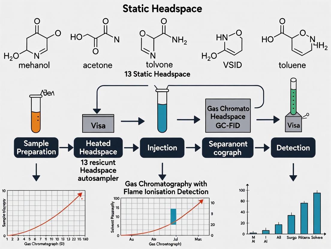
The following diagram illustrates the complete analytical procedure for residual solvent determination:

Diagram 1: Complete workflow for residual solvent analysis using static headspace GC-FID.

Research Reagent Solutions

Successful implementation of residual solvent methods requires specific, high-quality materials and reagents as detailed below:

Table 2: Essential Reagents and Materials for Residual Solvent Analysis

Reagent/Material	Specification	Function in Analysis
Reference Standards	USP Class 1, 2, and 3 solvent mixtures [1]	Quantification and identification of target solvents
Diluent	High-purity DMSO, DMA, or water [13] [14]	Sample dissolution while maintaining volatility
GC Column	6% cyanopropylphenyl/94% dimethylpolysiloxane (e.g., DB-624) [7] [13]	Separation of solvent mixtures
Carrier Gas	Helium or Nitrogen (99.999% purity) [7] [12]	Mobile phase for chromatographic separation
FID Gases	Hydrogen (fuel) and Zero Air (oxidizer) [12]	Maintaining stable flame for detection

Detailed Method Protocol

Sample Preparation Protocol

• Standard Solution Preparation: Accurately pipet reference solvents into a volumetric flask containing approximately 100 mL of dimethyl sulfoxide (DMSO) or N,N-dimethylacetamide (DMA). Bring to volume with diluent and mix thoroughly [13]. For working standards, dilute stock solution appropriately to match the expected concentration range of samples.

• Sample Solution Preparation: Precisely weigh approximately 100 mg of active pharmaceutical ingredient (API) into a headspace vial. Add 1.0 mL of diluent via pipette, immediately crimp seal the vial, and vortex until the sample is completely dissolved or uniformly suspended [13]. For drug products, crush tablets to a fine powder or empty capsule contents before weighing.

• System Suitability Solution: Prepare a mixture containing key solvents such as methyl ethyl ketone and ethyl acetate at their specification limits to verify chromatographic resolution ≥ 0.9 and injection precision (RSD ≤ 15.0%) [13].

Instrumental Parameters

The following diagram illustrates the key components and gas flow paths critical for proper FID operation:

Diagram 2: FID gas flow schematic and detection principle.

Table 3: Optimized GC-FID Instrument Parameters for Residual Solvent Analysis

Parameter	Setting	Rationale
Column	Elite-624 or DB-624, 30 m × 0.32 mm, 1.8 μm [7] [13]	Optimal for separating diverse solvent mixtures
Carrier Gas	Helium or Nitrogen at 1.5-2.0 mL/min [7] [12]	Maintains efficient separations
Oven Program	40°C (hold 10 min), ramp 10°C/min to 240°C [13]	Balances resolution and analysis time
Injector Temperature	140-150°C [13]	Ensures complete vaporization
Split Ratio	5:1 [14]	Prevents column overload
FID Temperature	250-280°C [7] [14]	Prevents condensation of combustion products
Hydrogen Flow	30-45 mL/min [10]	Optimal flame stability and sensitivity
Air Flow	300-450 mL/min [10]	Complete combustion for consistent response

Headspace Operating Conditions

• Equilibration Temperature: 80-120°C, optimized based on sample matrix and solvent volatility [13].
• Equilibration Time: 15-45 minutes to ensure complete partitioning between liquid and vapor phases [13].
• Loop/Syringe Temperature: 5-10°C above equilibration temperature to prevent condensation during transfer [1].
• Pressurization Time: 0.5-1.0 minute to ensure reproducible injection volumes [1].

Method Validation and Performance Data

Robust validation according to ICH guidelines demonstrates the reliability of HS-GC-FID methods for residual solvent analysis. The following performance characteristics are typically evaluated:

Table 4: Typical Validation Parameters for HS-GC-FID Residual Solvent Methods

Validation Parameter	Acceptance Criteria	Experimental Results
Specificity	No interference from sample matrix	Baseline resolution of all 13 target solvents [7]
Linearity	r² ≥ 0.999	r² = 0.9995 for acetone, THF, ethyl acetate [14]
Accuracy (Recovery)	90-110%	92.8-102.5% for seven solvents in linezolid [14]
Precision (Repeatability)	RSD ≤ 15%	RSD 0.4-0.8% for retention times and areas [14]
Limit of Quantitation	S/N ≥ 10	0.41 μg/mL (petroleum ether) to 11.86 μg/mL (DCM) [14]
Solution Stability	RSD ≤ 15% over 24-48 hours	Stable responses in DMSO for at least 48 hours [13]

Troubleshooting and Method Maintenance

Regular maintenance is essential for consistent FID performance. Key considerations include:

• Baseline Noise: Typically caused by contaminants in gas supplies or column bleed. Install high-purity gas filters and condition columns properly [9].
• Reduced Sensitivity: Often results from a partially clogged FID jet. Clean the jet every few weeks depending on sample load [9].
• Peak Tailing: Can indicate active sites in the inlet or column. Replace inlet liner and trim 10-15 cm from the column inlet [13].
• Irregular Retention Times: Usually caused by carrier gas flow fluctuations. Check for leaks and ensure pressure regulators are functioning properly [10].

Flame Ionization Detection remains the detection mechanism of choice for residual solvent analysis in pharmaceutical applications due to its exceptional reliability, sensitivity, and universal response to organic compounds. When coupled with static headspace sampling and appropriate chromatographic separation, GC-FID provides a robust, validated solution for compliance with stringent regulatory requirements. The protocols detailed in this application note provide a framework for implementing this powerful technique in pharmaceutical quality control laboratories, ensuring the safety of drug products by accurately monitoring potentially harmful solvent residues.

Residual solvents, classified as organic volatile impurities, are chemicals used or produced during the manufacture of drug substances, excipients, or drug products. These solvents provide no therapeutic benefit and may pose toxic risks to patients if not properly controlled and limited. Global regulatory frameworks, including the International Council for Harmonisation (ICH) Q3C guideline, the United States Pharmacopeia (USP) General Chapter <467>, and the European Pharmacopoeia, establish standardized requirements for residual solvent testing in pharmaceuticals. These regulations aim to ensure patient safety by limiting solvent exposure to toxicologically acceptable levels through scientifically valid analytical procedures [1] [15].

Gas chromatography (GC) represents the preferred analytical technique for residual solvents determination, with static headspace sampling coupled with flame ionization detection (HS-GC-FID) serving as the established methodology in pharmacopeial standards. This application note provides detailed guidance on regulatory requirements and experimental protocols for implementing static headspace GC-FID methods for residual solvent analysis, specifically contextualized within broader research on 13 target solvents.

ICH Q3C Guideline

The ICH Q3C guideline establishes a risk-based classification system for residual solvents based on their toxicity profiles:

• Class 1: Solvents to be avoided (known or suspected human carcinogens, environmental hazards)
• Class 2: Solvents to be limited (non-genotoxic animal carcinogens, neurotoxicants, teratogens)
• Class 3: Solvents with low toxic potential (PDE ≥ 50 mg/day) [16] [17]

The guideline establishes Permitted Daily Exposure (PDE) limits for Class 1 and Class 2 solvents, expressed in milligrams per day, which are converted to concentration limits in pharmaceutical products based on maximum daily dose. ICH Q3C applies to both new and existing pharmaceutical products, with recent updates addressing specific solvents such as ethylene glycol, which has a confirmed PDE of 6.2 mg/day (620 ppm) [16].

USP General Chapter <467>

USP <467> provides implemented testing procedures for assessing compliance with ICH Q3C limits, applying to all drug substances, excipients, and drug products covered by USP-NF monographs. The chapter specifies a three-step procedure for identifying and quantifying Class 1 and Class 2 solvents, utilizing static headspace GC-FID with two orthogonal stationary phases for identification, followed by quantitation [1] [15].

USP explicitly states that manufacturers may use alternative validated methods instead of the compendial procedures, provided these alternatives meet validation requirements and control objectives. This flexibility allows implementation of optimized methods for specific drug products while maintaining regulatory compliance [15].

European Pharmacopoeia

The European Pharmacopoeia contains harmonized requirements for residual solvents testing, with only minor methodological differences from USP <467>, primarily in reference standard mixtures and calculation approaches. Both pharmacopeias share common foundational principles and methodology despite these minor implementation variations [15].

Table 1: Residual Solvent Classification and Limits

Class	Basis for Classification	PDE Ranges	Example Solvents	Testing Requirements
Class 1	Known human carcinogens, strongly suspected human carcinogens, environmental hazards	Specific limits for each solvent	Benzene, Carbon tetrachloride, 1,1,1-Trichloroethane	Required, with strict controls
Class 2	Non-genotoxic animal carcinogens, neurotoxins, teratogens	PDE = 0.1 - 50 mg/day	Methanol, Chloroform, Toluene, Triethylamine, Ethylene glycol (PDE 6.2 mg/day)	Required, with concentration limits
Class 3	Low toxic potential, PDE ≥ 50 mg/day	PDE ≥ 50 mg/day	Ethanol, Ethyl acetate, Isopropyl alcohol	Required if cumulative >0.5%

Experimental Protocol: Static Headspace GC-FID Method

Materials and Equipment

Research Reagent Solutions

Table 2: Essential Materials and Reagents

Item	Function/Purpose	Specifications/Requirements
DB-624 Capillary Column	Separation of volatile solvents	30m × 0.25mm, 1.4μm film thickness; 6% cyanopropyl-phenyl/94% dimethyl polysiloxane [1]
Dimethyl Sulfoxide (DMSO)	Sample diluent	High-purity grade (99.9%), high boiling point (189°C) to minimize interference [6]
1,3-Dimethyl-2-imidazolidinone (DMI)	Alternative sample diluent	High boiling point (225°C), minimal interference, sharp solvent peak profile [17]
USP Reference Standards	System suitability, identification, quantitation	Class 1 Mixture, Class 2 Mixtures A, B, and individual solvent standards [1]
Helium or Hydrogen Carrier Gas	Mobile phase for chromatographic separation	Ultra-high purity grade; hydrogen provides optimal linear velocity [17]
Positive Displacement Pipettes	Accurate transfer of volatile standards	Essential for non-aqueous and volatile liquid transfers [17]

Instrumentation

• Gas Chromatograph: Agilent 7890A or equivalent, equipped with flame ionization detector [6]
• Headspace Sampler: Agilent 7697A or equivalent, with 1 mL sample loop [1]
• Analytical Column: Mid-polarity stationary phase such as DB-624 (6% cyanopropyl-phenyl/94% dimethyl polysiloxane) [1] [17]
• Data System: OpenLAB CDS or equivalent chromatography data system

Sample Preparation

Standard Solution Preparation

Prepare mixed standard solutions at concentrations corresponding to 100% of ICH Q3C specification limits:

• Stock Standard Preparation: Prepare individual solvent stock solutions in DMSO or DMI based on known densities and target concentrations [17]

• Working Standard Preparation: Combine appropriate volumes of stock solutions and dilute with DMSO to achieve final concentrations at specification limits. For a 10 g daily dose, prepare standards according to the following calculation:

  Standard Weight (mg) = (ICH Limit ppm × 50 mg/mL × 100 mL) / (400 × 1000) [17]

  Transfer 5.0 mL of working standard to 20 mL headspace vials, cap immediately, and crimp to ensure seal integrity [6]

Sample Solution Preparation

• Water-Soluble Materials: Dissolve 200 mg of test material in 5.0 mL of organic-free water [1]

• Water-Insoluble Materials: Dissolve 200 mg of test material in 5.0 mL of DMSO or DMI [6] [17]

• Vial Preparation: Transfer sample solution to 20 mL headspace vials, cap immediately, crimp, and mix using a vortex shaker for 1 minute [6]

Instrumental Parameters

Headspace Conditions

• Equilibration Temperature: 100°C [6]
• Equilibration Time: 30 minutes [6]
• Syringe Temperature: 105°C [6]
• Transfer Line Temperature: 110°C [6]
• Carrier Gas: Helium or Hydrogen, constant flow mode (4.7 mL/min for helium) [6]
• Pressurization Time: 1 minute [6]

GC-FID Conditions

• Injector Temperature: 190°C [6]
• Split Ratio: 1:5 to 50:1 (depending on solvent concentrations) [1] [6]
• Oven Temperature Program:
  • Initial: 40°C held for 5 minutes
  • Ramp 1: 10°C/min to 160°C
  • Ramp 2: 30°C/min to 240°C, held for 8 minutes [6]
• Total Run Time: 28 minutes [6]
• FID Temperature: 260°C [6]
• Hydrogen Air Flow: Optimized for maximum response (typically 30-40 mL/min)

Method Validation

Method validation should demonstrate suitability for intended purpose per regulatory requirements:

• Selectivity: No interference from diluent, sample matrix, or between target analytes [6]
• Linearity: Minimum correlation coefficient (r) of 0.999 over range of 10-120% of specification limits [6] [17]
• Accuracy: Recovery studies with spiked samples, acceptable range 90-110% [6]
• Precision: Repeatability (RSD ≤ 10.0%) and intermediate precision [6]
• Limit of Quantification (LOQ): Signal-to-noise ratio ≥ 10:1 at 10% of specification limit [6] [17]
• Robustness: Evaluation of method resilience to minor parameter variations [6]

Analytical Workflow

The following diagram illustrates the complete static headspace GC-FID analytical workflow for residual solvents determination:

Results and Discussion

Method Performance Characteristics

Validation studies demonstrate that the static headspace GC-FID method provides reliable performance for residual solvents determination:

• Linearity: Excellent linear response (r ≥ 0.999) across the concentration range of 10-120% of specification limits for all 13 target solvents [6] [17]

• Sensitivity: LOQ values below 10% of specification limits for all solvents, ensuring adequate detection capability at regulated levels [6]

• Precision: RSD values ≤ 10.0% for repeatability and intermediate precision studies, meeting acceptance criteria for robust quantitative analysis [6]

• Accuracy: Mean recovery values ranging from 95.98% to 109.40% across all target solvents, demonstrating minimal matrix effects [6]

Regulatory Compliance Strategy

Successful regulatory compliance requires a systematic approach to residual solvents control:

• Component-Based Testing: Test individual drug substance and excipients, or finished drug product, with justification for selected approach [15]

• Method Suitability: Demonstrate system suitability meeting resolution, tailing factor, and signal-to-noise requirements before sample analysis [6]

• Validation Documentation: Maintain comprehensive validation records demonstrating method reliability for intended applications [15]

• Change Control: Implement controlled procedures for method modifications with appropriate revalidation studies [15]

Static headspace GC-FID methodology provides a robust, reliable approach for determining residual solvents in pharmaceutical materials, enabling compliance with global regulatory requirements including ICH Q3C, USP <467>, and European Pharmacopoeia standards. The experimental protocols detailed in this application note establish a validated framework for simultaneous identification and quantification of 13 target residual solvents, with demonstrated linearity, precision, accuracy, and sensitivity meeting regulatory expectations.

Implementation of this standardized methodology across pharmaceutical development and quality control laboratories can significantly reduce method development time while ensuring patient safety through reliable control of potentially toxic solvent residues. The flexibility afforded by regulatory authorities for use of validated alternative methods enables continuous improvement of analytical approaches while maintaining compliance with quality requirements.

Static Headspace Gas Chromatography with Flame Ionization Detection (HS-GC-FID) has emerged as a superior technique for monitoring residual solvents in pharmaceutical products, offering significant advantages over both direct injection GC-FID and GC-mass spectrometry (GC-MS) for this specific application. Residual solvents, classified as organic volatile impurities in active pharmaceutical ingredients (APIs) and finished drug products, require precise monitoring to comply with stringent International Council for Harmonisation (ICH) Q3C and United States Pharmacopeia (USP) <467> guidelines [13] [18]. These regulations mandate limits on Class 1 (solvents to be avoided), Class 2 (solvents to be limited), and Class 3 (solvents with low toxic potential) solvents to ensure patient safety [18]. This application note demonstrates, within the context of research on 13 residual solvents, how HS-GC-FID provides an optimal balance of sensitivity, robustness, and efficiency for regulated pharmaceutical analysis.

Theoretical Advantages of HS-GC-FID

Fundamental Principles of Static Headspace Analysis

Static headspace sampling operates on the principle of partitioning volatile analytes between a sample matrix (liquid or solid) and the gas phase (headspace) in a sealed vial [19]. At equilibrium, the concentration of a volatile solvent in the gas phase is proportional to its original concentration in the sample, allowing for quantitative analysis [13]. This equilibrium is governed by the partition coefficient (K), defined as K = C~S~/C~G~, where C~S~ is the concentration in the sample phase and C~G~ is the concentration in the gas phase [13]. The fundamental relationship in static headspace analysis shows that the chromatographic peak area is proportional to the original analyte concentration and inversely proportional to (K + β), where β is the phase ratio (V~G~/V~S~) of the headspace vial [13].

The selection of an analytical technique for residual solvents depends on the sample matrix, required sensitivity, and regulatory constraints. Direct injection introduces the sample solution directly into the GC inlet, while headspace sampling analyzes the equilibrated vapor phase [20]. GC-MS provides compound identification via mass spectra but can present quantification challenges at low concentrations [1].

Experimental Protocols

Generic HS-GC-FID Method for 13 Residual Solvents

3.1.1 Materials and Reagents

• Diluent: N,N-Dimethylacetamide (DMA) or Dimethyl sulfoxide (DMSO), spectrophotometry grade or HSGC grade [13] [6]. High-boiling, aprotic solvents minimize interference and effectively dissolve API samples.
• Reference Standards: Individual or mixed residual solvent standards at GC or HPLC grade. Common solvents include methanol, ethanol, acetone, ethyl acetate, isopropanol, dichloromethane, n-hexane, tetrahydrofuran, chloroform, toluene, and others as required [13] [21].
• API Samples: Approximately 100 mg of active pharmaceutical ingredient, accurately weighed [13].
• Gas Supplies: Ultra-high-purity hydrogen or helium as carrier gas, nitrogen or hydrogen for FID make-up gas, zero air for FID [13] [22].

Table 1: Research Reagent Solutions for HS-GC-FID Residual Solvent Analysis

Item	Function	Key Specifications
DMA (N,N-Dimethylacetamide)	Sample diluent	High boiling point (165°C), aprotic, effectively dissolves APIs, minimizes volatile interference [13]
Residual Solvent Standards	Calibration and quantification	GC/HPLC grade, certified for concentration and identity [13]
Internal Standard (n-propanol)	Quantification control	Corrects for injection volume variability; not present in samples [23]
Hydrogen/Helium Gas	GC Carrier gas	Ultra-high purity (99.999%) to maintain column performance and detector stability [22]
Zero Air	FID Oxidant	Hydrocarbon-free (<0.1 ppm) for low baseline noise and high sensitivity [23]

3.1.2 Instrumentation and Conditions

Table 2: Standard HS-GC-FID Operating Conditions [13] [22] [6]

Parameter	Setting	Alternative/Fast Method
GC System	Agilent 7890/6890 or equivalent	Scion 8300 GC or equivalent
Headspace Sampler	Agilent G1888 or equivalent	CTC PAL System or equivalent
Column	DB-624, 30 m × 0.32 mm, 1.8 µm	Rtx-624, 30 m × 0.25 mm, 1.4 µm
Carrier Gas	Hydrogen or Helium	Hydrogen
Flow Rate	1.5 mL/min (constant flow)	2.0 mL/min
Injector Temperature	140-190°C	280°C
Split Ratio	5:1	10:1
Oven Program	40°C (hold 20 min) → 10°C/min → 240°C (hold 20 min)	30°C (hold 6 min) → 15°C/min → 85°C (hold 2 min) → 35°C/min → 250°C
FID Temperature	250-260°C	320°C
Headspace Incubation	80-100°C	80°C
Headspace Equilibration	30-45 min	45 min
Syringe Temperature	105-110°C	150°C
Transfer Line	110-170°C	170°C

3.1.3 Sample Preparation Protocol

• Standard Solution:

  • Prepare a stock standard solution by accurately pipetting appropriate volumes of each neat solvent into a 250 mL volumetric flask containing approximately 100 mL of DMA [13].
  • Bring to volume with DMA and mix well. Critical: Pipette volatile solvents directly into diluent to prevent evaporation losses [13].
  • Serially dilute to create working standards covering the required concentration range (typically from LOQ to 150% of specification limits).

• Sample Solution:

  • Accurately weigh approximately 100 mg of API into a 10-20 mL headspace vial [13].
  • For low-availability compounds (NCEs), sample amounts can be reduced to 10-50 mg [13].
  • Pipette 1.0 mL of DMA into the vial and immediately seal with a PTFE-lined crimp cap.
  • Vortex until the sample is completely dissolved or finely suspended. Note: Sonication is not recommended as it may promote degradation [13].

• System Suitability Solution:

  • Prepare a solution containing key solvent pairs (e.g., methyl ethyl ketone/ethyl acetate) at the 100% limit concentration to verify chromatographic resolution ≥ 0.9 [13].
  • Prepare a sensitivity check solution at the LOQ level to ensure signal-to-noise ratio ≥ 10:1 [13].

3.1.4 Analysis Sequence and Quantitation

• Injection Sequence: Blank → Sensitivity solution → Working standard (6 replicates) → Blank → Samples (single injection per preparation) [13].
• System Suitability Criteria:
  • Blank: No interfering peaks at target analyte retention times.
  • Resolution: Rs ≥ 0.9 between critical pairs.
  • Precision: RSD ≤ 15.0% for six replicate standard injections.
  • Sensitivity: S/N ≥ 10 for each peak in the sensitivity solution [13].
• Quantitation: Use external standardization, calculating solvent concentration in the sample based on peak area, standard concentration, and sample weight [13].

Results and Discussion

Performance Comparison of Analytical Techniques

Table 3: Quantitative Comparison of HS-GC-FID, Direct Injection, and GC-MS

Parameter	HS-GC-FID	Direct Injection GC-FID	GC-MS
Sample Introduction	Vapor phase only	Liquid sample	Liquid or vapor phase
Matrix Effects	Minimal for volatiles	Significant, non-volatiles deposit in inlet	Significant, ion suppression possible
Sensitivity for Volatiles	Excellent (ppb-ppm)	Good (ppm)	Good (ppm) but can be limited for quantitation [1]
System Robustness	High (no non-volatile contamination)	Low (frequent inlet/column maintenance)	Moderate (source contamination)
Sample Preparation	Minimal (dissolve and inject)	May require filtration, dilution	May require filtration, dilution
Analysis Time	Moderate (includes equilibration)	Fast (no equilibration)	Moderate to fast
Identification Certainty	Retention time only	Retention time only	Spectral confirmation [1]
Ideal For	Routine analysis of volatile impurities	Samples free of non-volatiles	Unknown identification, research
Regulatory Acceptance	High (USP <467>)	Moderate	High (with proper validation)

Case for HS-GC-FID Over Alternative Techniques

4.2.1 HS-GC-FID vs. Direct Injection

Headspace sampling provides superior robustness for pharmaceutical analysis by introducing only volatile compounds into the GC system, preventing non-volatile API components from contaminating the inlet and column [20] [21]. This is particularly crucial for analyzing complex drug substances where non-volatile matrix components can degrade system performance [21]. Direct injection of API solutions often leads to significant maintenance downtime and variable performance [21]. Furthermore, headspace sampling minimizes sample preparation, as filtration is unnecessary and complex matrices can often be analyzed as suspensions rather than complete solutions [13] [20].

4.2.2 HS-GC-FID vs. GC-MS

While GC-MS provides powerful identification capability through spectral matching, HS-GC-FID offers practical advantages for routine quantitative analysis of known residual solvents. FID demonstrates a wide linear dynamic range (typically 10^4-10^6) and consistent response factors for carbon-containing compounds, making it ideal for quantifying solvents at diverse concentration levels [13]. MS detection can face quantification challenges near the limit of permissible concentrations due to split flow requirements and potential sensitivity issues in full-scan mode [1]. Additionally, HS-GC-FID systems have lower acquisition and maintenance costs, making them more accessible for quality control laboratories performing high-volume testing. For regulated methods where target analytes are known, the spectral identification provided by MS may be unnecessary, and FID delivers sufficient confirmation through retention time matching with standards [1].

Method Validation and Application

A properly validated HS-GC-FID method demonstrates excellent precision, accuracy, and sensitivity for residual solvent analysis. Validation data for pharmaceutical applications typically shows relative standard deviations (RSD) ≤ 15.0% for system precision, average recoveries of 95-109% for accuracy, and limits of quantification (LOQ) well below ICH specification limits [13] [6]. The technique has been successfully applied to various drug substances, including losartan potassium, where it detected isopropyl alcohol and triethylamine as residual solvents from the synthesis process [6]. The generic nature of the method allows for adaptation to new chemical entities with minimal modification, primarily through optimization of diluent selection and headspace equilibrium conditions to address solubility or stability issues [13] [6].

For the quantitative analysis of 13 residual solvents in pharmaceutical products, static HS-GC-FID represents the optimal analytical technique, balancing regulatory compliance, analytical performance, and operational practicality. Its superiority over direct injection GC-FID lies in its exceptional robustness and minimal sample preparation, while its advantage over GC-MS comes from its reliable quantification performance and accessibility for quality control environments. The detailed protocols provided herein enable reliable method implementation, ensuring patient safety through accurate monitoring of these potentially toxic impurities in accordance with ICH Q3C and USP <467> guidelines.

In the pharmaceutical industry, residual solvents are defined as organic volatile chemicals that are used or produced in the manufacture of drug substances or excipients, or in the preparation of drug products [24]. Since these solvents are not completely removed by practical manufacturing techniques, they may remain in final pharmaceutical products, potentially posing safety risks to patients. The International Council for Harmonisation (ICH) developed the Q3C guideline to provide recommendations on the use of less toxic solvents and to establish acceptable exposure limits for residual solvents in pharmaceuticals based on toxicological data [16] [24].

The ICH Q3C guideline categorizes residual solvents into three classes based on their toxicity and health risks [24]. This classification system provides a structured framework for controlling these impurities in pharmaceutical products, ensuring patient safety while recognizing the practical necessities of pharmaceutical manufacturing. The guidance emphasizes that drug products should contain no higher levels of residual solvents than can be supported by safety data, making accurate classification and quantification essential throughout drug development [25].

ICH Solvent Classification System

Classification Categories

The ICH Q3C guideline establishes a three-class system for categorizing residual solvents based on their toxicity profiles [24]:

• Class 1 solvents: Solvents to be avoided - Known human carcinogens, strongly suspected human carcinogens, and environmental hazards.
• Class 2 solvents: Solvents to be limited - Non-genotoxic animal carcinogens or possible causative agents of other irreversible toxicity such as neurotoxicity or teratogenicity. Also includes solvents suspected of other significant but reversible toxicities.
• Class 3 solvents: Solvents with low toxic potential - Solvents with low toxic potential to man; no health-based exposure limit is needed. Class 3 solvents have PDEs of 50 mg or more per day.

Quantitative Limits for Residual Solvents

The ICH Q3C guideline establishes Permitted Daily Exposure (PDE) limits for residual solvents, which represent the maximum acceptable intake per day without significant risk to patient health [16] [24]. These PDE values are derived from toxicological data, typically by dividing the most appropriate No-Observed-Adverse-Effect-Level (NOAEL) from animal studies by a set of uncertainty factors [25]. For most solvents, the guideline also provides concentration limits based on the assumption of a daily drug intake of 10 grams [24].

Table 1: ICH Q3C Classification of Residual Solvents and Their Limits

Solvent	ICH Class	PDE (mg/day)	Concentration Limit (ppm)
Benzene	1	-	2
Carbon tetrachloride	1	-	4
1,2-Dichloroethane	1	-	5
1,1-Dichloroethene	1	-	8
1,1,1-Trichloroethane	1	-	1500
Acetonitrile	2	4.1	410
Chloroform	2	0.6	60
Cyclohexane	2	38.8	3880
Dichloromethane	2	6.0	600
Ethylene glycol	2	6.2	620
Formamide	2	2.2	220
Hexane	2	2.9	290
Methanol	2	30.0	3000
N-Methylpyrrolidone	2	5.3	530
Tetrahydrofuran	2	7.2	720
Toluene	2	8.9	890

Table 2: Class 3 Solvents with Low Toxic Potential

Solvent	ICH Class	PDE (mg/day)
Acetone	3	50
Ethyl acetate	3	50
Ethanol	3	50
Heptane	3	50

Regulatory Context and Recent Developments

Harmonization of ICH Q3C and USP <467>

While ICH Q3C applies specifically to new drug products, the United States Pharmacopeia (USP) general chapter <467> Residual Solvents applies the same requirements to all new and existing drug products [24]. This harmonization in approach, with the notable exception of scope, ensures consistent safety standards across the pharmaceutical industry. Regulatory authorities require manufacturers to demonstrate compliance with these residual solvent limits through validated analytical methods [24].

Historical Perspective on Ethylene Glycol Limits

The evolution of safety limits for specific solvents demonstrates the dynamic nature of residual solvent regulations. A notable example is ethylene glycol, which experienced a correction in its established PDE. Prior to 2017, ICH Q3C listed ethylene glycol as a Class 2 residual solvent with a PDE of 6.2 mg/day [16]. In 2017, a discrepancy was identified between Summary Table 2 of the guideline (6.2 mg/day) and the monograph in Appendix 5 (3.1 mg/day) [16]. After investigation, archival documents revealed that the 6.2 mg/day value had been accepted following a reassessment of toxicity data in 1997, but the Appendix had not been updated accordingly [16]. The original PDE of 6.2 mg/day was reinstated in the current version of the guideline [16].

Ongoing Re-evaluation of Class 1 Solvents

Despite multiple revisions to ICH Q3C, the PDE limits for Class 1 solvents have remained unchanged since originally proposed in 1997 [25]. Recent scientific literature has called for a re-evaluation of these limits based on new toxicological data that has become available over the past decades [25]. A detailed review of current information suggests that there is a case for changing limits for all Class 1 solvents except benzene [25]. It has been proposed that the limits for carbon tetrachloride, 1,2-dichloroethane, and 1,1-dichloroethene could be increased, while the limit for 1,1,1-trichloroethane should be reduced [25].

Analytical Methodologies for Residual Solvent Analysis

Headspace Gas Chromatography Techniques

The analysis of residual solvents in pharmaceuticals is typically performed using headspace gas chromatography (GC), often coupled with flame ionization detection (FID) or mass spectrometry (MS) [24] [14]. The static headspace technique is particularly advantageous for volatile organic compounds as it involves sampling the vapor phase in equilibrium with the solid or liquid sample in a sealed vial [14]. This approach minimizes the introduction of non-volatile matrix components that could contaminate the GC system or interfere with analysis [14].

Table 3: Research Reagent Solutions for Residual Solvent Analysis

Reagent/Material	Function/Application
ZB-WAX or DB-FFAP Capillary Column	GC separation of polar solvents
Dimethyl Sulfoxide (DMSO)	Sample solvent for insoluble APIs
Headspace Grade Solvents	Low impurity background for trace analysis
Valve-and-Loop Headspace Autosampler	Automated, precise sample introduction
Nitrogen Carrier Gas (99.999%)	Mobile phase for GC separation

Method Validation Parameters

For regulatory compliance, analytical methods for residual solvent determination must be properly validated. Key validation parameters include [14]:

• Linearity: Demonstrated by correlation coefficient (r) greater than 0.9995 for most solvents [14]
• Precision: Both run-to-run and day-to-day assay precision with relative standard deviation (RSD) typically below 1.3% [14]
• Accuracy: Recovery rates ranging from 92.8% to 102.5% for validated methods [14]
• Sensitivity: Limits of detection (LOD) and quantitation (LOQ) determined at signal-to-noise ratios of 3:1 and 10:1, respectively [14]

Figure 1: Static Headspace GC-FID Workflow for Residual Solvent Analysis

Experimental Protocol: Static Headspace GC-FID for Residual Solvents

Materials and Equipment

• Gas Chromatograph: Agilent 7890A GC system or equivalent with FID [14]
• Headspace Autosampler: TriPlus 500 or equivalent with valve-and-loop technology [24]
• Capillary Column: ZB-WAX or DB-FFAP (30 m × 0.53 mm i.d., 1.0 µm film thickness) [14]
• Chemicals: Headspace grade solvents and diluents (DMSO, water, DMF, DMAC) [24]
• Reference Standards: Certified reference materials for all target solvents [14]

Sample Preparation Protocol

• Standard Solution Preparation: Accurately weigh reference substances and dissolve in appropriate diluent (e.g., DMSO) to prepare stock solutions [14]. Store in dark glass vials at 4°C.
• Working Solution Preparation: Freshly prepare working solutions by serial dilution of stock solutions on the day of analysis [14].
• Sample Solution Preparation: Accurately weigh approximately 100 mg of drug substance (linezolid or equivalent) and dissolve in 5.0 mL of DMSO in a 20 mL headspace vial [14].
• Vial Sealing: Immediately seal vials with PTFE-faced silicone septa and crimp caps to prevent solvent loss [14].

Instrumental Parameters

• Headspace Conditions: [14]
  • Oven temperature: Appropriate based on solvent volatility
  • Loop temperature: Maintained above oven temperature
  • Transfer line temperature: Optimized to prevent condensation
• GC Conditions: [14]
  • Carrier gas: Nitrogen (99.999% purity) at 1 mL/min constant flow
  • Injector temperature: 90°C with split ratio 5:1
  • Oven program: Initial 30°C for 15 min, ramp at 10°C/min to 35°C hold 10 min, then 30°C/min to 220°C hold 30 min
  • FID temperature: 280°C
  • Hydrogen, air, and makeup gas flows optimized for maximum response

Method Validation Steps

• System Suitability: Verify resolution, peak symmetry, and retention time reproducibility before sample analysis [14]
• Linearity Assessment: Analyze at least five concentration levels for each solvent with r > 0.999 [14]
• Precision Determination: Perform six replicate injections of standard solutions with RSD < 1.5% [14]
• Accuracy Evaluation: Spike recovery experiments at 50%, 100%, and 150% of target concentration [14]

The ICH Q3C guideline provides a scientifically rigorous framework for classifying residual solvents and establishing safety-based limits that protect patient health while recognizing the practical realities of pharmaceutical manufacturing. The classification into Class 1 (solvents to be avoided), Class 2 (solvents to be limited), and Class 3 (solvents with low toxic potential) enables risk-based approach to solvent selection and control strategies [24].

Static headspace GC-FID methodology has proven to be a robust and sensitive technique for monitoring compliance with ICH Q3C limits, particularly when analyzing multiple solvent residues in complex pharmaceutical matrices [14]. The experimental protocol outlined in this application note provides researchers with a validated approach for determining residual solvents in active pharmaceutical ingredients, supporting quality control in drug development and manufacturing.

As toxicological science advances, continued evolution of residual solvent limits is expected, particularly for Class 1 solvents where recent research suggests current limits may require revision based on new data and assessment methodologies [25]. Pharmaceutical scientists must therefore remain current with both regulatory requirements and analytical technologies to ensure patient safety while facilitating efficient drug development.

A Step-by-Step Guide to Developing and Implementing Your HS-GC-FID Method

Static headspace gas chromatography coupled with flame ionization detection (HS-GC-FID) is a widely established technique for determining residual solvents in active pharmaceutical ingredients (APIs) and drug products. The reliability of this analysis critically depends on the optimal configuration of instrumental parameters, particularly the GC oven program, injector, and FID temperatures. These parameters directly influence key performance metrics including resolution, sensitivity, analysis time, and reproducibility. This application note provides a comprehensive overview of evidence-based parameter settings and detailed protocols tailored for researchers and drug development professionals engaged in residual solvent analysis, framed within a broader thesis investigating 13 residual solvents.

Critical Instrumental Parameters and Comparative Data

Optimal configuration of the gas chromatograph is fundamental for achieving efficient separation, sharp peak shapes, and robust quantification. The table below summarizes two distinct sets of proven instrumental parameters for residual solvent analysis, demonstrating the balance between analysis time and chromatographic performance.

Table 1: Comparative HS-GC-FID Instrumental Parameters for Residual Solvent Analysis

Parameter	Conventional USP-style Method [22]	Fast GC Method [22]	Losartan Potassium Method [6]	Suvorexant Method [26]
Column	Rtx-624, 30 m x 0.25 mm, 1.40 µm	Rtx-624, 30 m x 0.25 mm, 1.40 µm	DB-624, 30 m x 0.53 mm, 3.0 µm	DB-624, 30 m x 0.53 mm, 3.0 µm
Carrier Gas & Flow	Hydrogen, 1.5 mL/min	Hydrogen, 2.0 mL/min	Helium, 4.718 mL/min	Not Specified
Split Ratio	5:1	10:1	1:5	Not Specified
Injector Temp.	140 °C	280 °C	190 °C	220 °C
FID Temp.	250 °C	320 °C	260 °C	280 °C
Oven Program	40 °C (hold 20 min)10 °C/min to 240 °C (hold 20 min)	30 °C (hold 6 min)15 °C/min to 85 °C (hold 2 min)35 °C/min to 250 °C (hold 0 min)	40 °C (hold 5 min)10 °C/min to 160 °C30 °C/min to 240 °C (hold 8 min)	Programmed Temperature
Headspace Incubation	80 °C for 45 min	80 °C for 45 min	100 °C for 30 min	Not Specified
Total Run Time	~60 minutes	~16.5 minutes	~28 minutes	Not Specified

Parameter Selection Rationale

• Oven Temperature Program: The initial temperature and hold time are critical for resolving highly volatile solvents. The conventional method uses a 20-minute isothermal hold at 40°C for this purpose [22]. In contrast, faster ramps (15-35°C/min) are employed in accelerated methods to reduce runtime while maintaining resolution for mid- and high-boiling solvents [22].
• Injector Temperature: Must be sufficiently high to ensure immediate vaporization of the transferred headspace vapor without causing thermal degradation. A wide range (140°C to 280°C) is successfully used, often balanced against the split ratio and carrier flow [22] [6] [26].
• FID Temperature: Typically set at least 20-50°C above the final oven temperature to prevent condensation of high-boiling analytes and ensure a stable baseline. The FID temperature for residual solvents commonly ranges from 250°C to 320°C [22] [26].

Experimental Protocol: A Step-by-Step Workflow

The following diagram and protocol outline the complete workflow for determining residual solvents using static HS-GC-FID.

Detailed Procedures

Sample and Standard Preparation

• Select Diluent: Choose a high-boiling, low-volatility solvent. Dimethyl sulfoxide (DMSO) and 1,3-Dimethyl-2-imidazolidinone (DMI) are preferred for their ability to dissolve a wide range of APIs and their high boiling points which minimize interference [6] [17].
• Prepare Standard Solutions:
  • Prepare a mixed stock standard containing all target residual solvents at concentrations based on their ICH Q3C(R8) specification limits [17].
  • Use positive displacement pipettes for accurate and reproducible transfer of volatile organic standards [17].
  • A typical working standard is prepared by diluting the stock standard with the selected diluent. For example, dilute 4.0 mL of mixed stock standard to 100 mL with DMI [17].
• Prepare Sample Solution:
  • Accurately weigh approximately 50 mg/mL of the API into a headspace vial [17].
  • Add 5.0 mL of the selected diluent, cap the vial immediately, and crimp to ensure a tight seal [6].

Headspace and GC-FID Analysis

• Load Vials: Place prepared standard and sample vials into the headspace autosampler tray.
• Set Headspace Conditions:
  • Incubation Temperature: Typically 80°C to 100°C. Higher temperatures increase the partitioning of analytes into the headspace but must be kept about 20°C below the diluent's boiling point [6] [27].
  • Incubation Time: 30 to 45 minutes to ensure equilibrium is reached between the sample solution and the headspace vapor [22] [6].
  • Syringe/Transfer Line Temperature: Set 5-10°C above the incubation temperature (e.g., 105°C) to prevent condensation [22] [6].
• Configure GC Parameters:
  • Follow the parameters detailed in Table 1 for the chosen method (e.g., Conventional vs. Fast GC).
  • Ensure the FID gas flows (Hydrogen, Air, and make-up gas like Nitrogen) are optimized according to the manufacturer's recommendations for stable detection.
• Execute Sequence: Run the analytical sequence, typically starting with a diluent blank, followed by standard solutions, and then the unknown samples.

The Scientist's Toolkit: Essential Research Reagents and Materials

The following table lists key materials required for establishing a robust HS-GC-FID method for residual solvents.

Table 2: Essential Research Reagents and Materials for HS-GC-FID Analysis

Item	Function & Importance	Examples / Specifications
GC Capillary Column	Stationary phase for chromatographic separation of volatiles.	DB-624 or Rtx-624 (6% cyanopropylphenyl / 94% dimethyl polysiloxane); 30 m length; 0.25-0.53 mm ID; 1.4-3.0 µm film thickness [22] [6] [26].
High-Purity Diluent	Dissolves the API without interfering in the analysis; high boiling point is critical.	Dimethyl Sulfoxide (DMSO), 1,3-Dimethyl-2-imidazolidinone (DMI), or organic-free water [6] [17].
Reference Standards	For peak identification and quantitation.	USP Class 1 and Class 2 Residual Solvent Mixtures, or individual certified solvent standards [1] [17].
Headspace Vials & Closures	Contain the sample and maintain a pressurized, sealed system for vapor equilibration.	10 mL or 20 mL vials with PTFE/silicone septa and aluminum crimp caps [27].
Positive Displacement Pipette	Ensures accurate and precise transfer of volatile liquid standards, minimizing evaporation loss.	[17]
High-Purity Gases	Carrier gas for GC and detector gases for FID.	Hydrogen or Helium (carrier grade), Hydrogen (FID fuel), Zero Air (FID oxidizer) [22] [6].

This application note synthesizes current methodologies and provides detailed protocols for optimizing the core instrumental parameters in HS-GC-FID analysis of residual solvents. The comparative data demonstrates that method parameters can be successfully adjusted to prioritize either high-resolution, pharmacopeia-compliant results or faster analysis times to meet throughput demands. The provided experimental workflow and toolkit offer a solid foundation for researchers to develop, validate, and transfer robust analytical methods that ensure patient safety and regulatory compliance in pharmaceutical development.

The accurate quantification of residual solvents in active pharmaceutical ingredients (APIs) is a critical requirement in pharmaceutical development, mandated by global regulatory standards. Static headspace gas chromatography with flame ionization detection (HS-GC-FID) serves as the cornerstone technique for this analysis. A fundamental challenge in this process is the selection of an appropriate sample diluent, which must completely dissolve the often poorly water-soluble API while simultaneously enabling the efficient partitioning of volatile analytes into the gas phase for measurement. This application note details the strategic use of dipolar aprotic solvents—specifically dimethyl sulfoxide (DMSO), N,N-dimethylformamide (DMF), and N,N-dimethylacetamide (DMA)—and their mixtures with water to overcome solubility limitations, thereby ensuring robust, accurate, and sensitive analytical methods.

The Scientific Rationale for Diluent Selection

The core challenge in headspace analysis lies in the conflicting requirements of sample solubility and analyte volatility. While water is a clean, stable, and inexpensive diluent, its use limits the headspace equilibration temperature to below 100 °C to avoid dangerous pressure buildup, which can result in poor volatilization for many high-boiling point Class 2 residual solvents [28]. Furthermore, a significant number of synthetic drug substances exhibit low solubility in pure water.

Dipolar aprotic solvents offer a powerful solution to this dilemma. Their high polarity and ability to dissolve a wide range of organic compounds make them exceptional diluents for complex APIs. Moreover, their high boiling points (DMSO: 189 °C, DMF: 153 °C, DMA: 166 °C) permit incubation at elevated temperatures, significantly enhancing the transfer of higher-boiling solvents into the headspace [8] [28]. The molecular interactions within these solvents, including strong dipole-dipole interactions and their ability to act as hydrogen-bond acceptors, are key to their dissolution prowess [29]. When mixed with water, these solvents can form unique solvent systems that further fine-tune solubility and volatility characteristics, providing a versatile toolkit for the analytical scientist.

Comparative Analysis of Diluent Properties

Selecting the optimal diluent or diluent mixture requires a clear understanding of the physicochemical properties of each candidate. The table below provides a comparative overview of DMSO, DMF, and DMA.

Table 1: Key Properties of Dipolar Aprotic Diluents for Headspace Analysis

Property	DMSO	DMF	DMA	Water	Significance for HS-GC
Boiling Point (°C)	189 [8]	153 [30]	166 [30]	100	Determines maximum safe incubation temperature.
Dielectric Constant	46.7 [29]	36.7 [29]	37.6 [29]	~80	Indicates solvent polarity and dissolution capability.
Dipole Moment (D)	3.96 [29]	3.74 [29]	3.16 [29]	1.85	Influences molecular interactions with API and solvents.
Common Applications	Solvent for APIs, polymers, and salts [29] [30]	Widely used in industrial processes [29]	Used in polymer dissolution and synthesis [29] [30]	Universal solvent	Versatility in dissolving diverse analytes.

The following diagram illustrates the logical decision-making process for selecting an appropriate diluent based on API solubility, which directly addresses the core challenge outlined in this note.

The Scientist's Toolkit: Essential Research Reagents

Successful method development relies on a set of core reagents and materials. The following table lists the essential components for developing a residual solvent method using the diluents discussed.

Table 2: Essential Research Reagents and Materials for Method Development

Item	Function/Purpose	Key Considerations
DMSO, DMF, DMA	High-boiling diluents for dissolving poorly water-soluble APIs.	Use high-purity grade (e.g., ≥99.9%); dry with molecular sieves if necessary [8] [30].
Internal Standard (e.g., ¹³C₇-Toluene)	Added to sample to correct for variability in headspace injection and sample preparation [28].	Must be well-resolved, chemically similar to analytes, and not present in the sample.
DB-624 Capillary Column	Standard stationary phase for separating volatile organic compounds.	Common dimensions: 30 m x 0.32/0.53 mm, 1.8-3.0 µm film thickness [1] [28].
USP Class 1 & 2 RS Standards	Reference standards for identification and quantitation of target solvents.	Used to prepare calibration solutions and for system suitability testing [1].

Detailed Experimental Protocol

This protocol provides a step-by-step guide for developing and executing a static headspace GC-FID method for the determination of 13 residual solvents in a poorly water-soluble API, using DMSO as a model diluent.

Materials and Equipment

• Gas Chromatograph: Agilent 6890N or equivalent, equipped with an FID.
• Headspace Sampler: Agilent 7694 or equivalent.
• Column: DB-624 capillary column (30 m × 0.53 mm i.d., 3.00 µm film thickness) [28].
• Chemicals: High-purity DMSO; USP-grade residual solvent reference standards; API sample.

Stock and Standard Solution Preparation

• Stock Standard Solution: Accurately weigh and combine the 13 target residual solvents in DMSO to prepare a concentrated stock solution.
• Internal Standard Solution: Prepare a solution of a suitable internal standard (e.g., 1-pentanol or acetonitrile-d₃) in DMSO at a concentration near the midpoint of the calibration curve.
• Calibration Standards: Dilute the stock standard solution with DMSO to create a series of calibration standards spanning the range from the quantitation limit (QL) to 120% of the specified limit for each solvent. For a limit of 5000 ppm, this would typically be from QL to 6000 ppm [31]. Add a constant volume of the internal standard solution to each calibration level.
• Sample Solution: Accurately weigh approximately 100 mg of the API into a headspace vial. Add 1.0 mL of DMSO containing the internal standard at the same concentration as in the calibration standards. Seal the vial immediately with a crimp cap.

Instrumental Parameters

The following optimized conditions, derived from a central composite experimental design, are recommended as a starting point [28]:

• GC Inlet: Split mode (5:1 ratio), temperature: 140 °C.
• Carrier Gas: Helium or Nitrogen, constant flow at 1.90 mL/min.
• Oven Temperature Program:
  • Initial Temperature: 30 °C
  • Ramp: 10 °C/min
  • Final Temperature: 158 °C
  • Hold Time: 5 min
• FID Temperature: 250 °C.
• Headspace Conditions:
  • Oven Temperature: 90-110 °C (can be optimized based on solvent volatility)
  • Loop Temperature: 110 °C
  • Transfer Line Temperature: 120 °C
  • Vial Equilibration Time: 30-45 minutes
  • Vial Pressurization: 15-20 psi

Analysis and Quantitation

• Inject 1.0 mL of the headspace gas from each vial.
• Process the data by plotting the peak area ratio (analyte to internal standard) against the concentration of each calibration standard.
• Use the resulting linear calibration curve to calculate the concentration of each residual solvent in the API sample.

Method Validation Considerations

To ensure regulatory compliance, the developed method must be validated per ICH guidelines. Key validation parameters include:

• Specificity: Ensure no interference from the API or diluent at the retention times of the target solvents and internal standard.
• Linearity and Range: Demonstrate a linear response from the QL to 120% of the specification limit, with a correlation coefficient (r) of ≥0.990 [31].
• Accuracy (Recovery): Perform spike recovery experiments by spiking the API with residual solvents at three concentration levels (e.g., 50%, 100%, and 150% of the specification limit) in triplicate. Acceptable recovery is typically 80-120% for each level [31].
• Precision: Establish repeatability by analyzing six independently prepared samples spiked at 100% of the limit. The relative standard deviation (RSD) should be ≤15%.
• Robustness: Deliberately vary critical method parameters (e.g., carrier gas flow rate ±0.1 mL/min, initial oven temperature ±2 °C) to demonstrate the method's resilience [31].

The strategic selection of DMSO, DMF, DMA, or their aqueous mixtures as diluent is a powerful approach to overcoming the pervasive challenge of API solubility in residual solvents analysis by static headspace GC-FID. By enabling the complete dissolution of the sample and permitting higher headspace incubation temperatures, these solvents facilitate the accurate and sensitive detection of a wide range of volatile impurities. The detailed protocols and comparative data provided in this application note empower scientists to make informed decisions during method development, leading to robust, reliable, and regulatory-compliant analytical procedures that are critical for ensuring drug safety and quality.

Proper sample preparation is a foundational pillar for achieving accurate, reproducible, and reliable results in static headspace gas chromatography with flame ionization detection (HS-GC-FID). This process is particularly critical in the pharmaceutical industry for the analysis of 13 common residual solvents, including methanol, ethanol, acetone, acetonitrile, tetrahydrofuran, dichloromethane, and others, in various nanoformulations and drug substances [7]. Even the most advanced instrumental analysis cannot compensate for errors introduced during sample weighing, dilution, or vial sealing. Meticulous preparation directly influences key analytical outcomes such as sample integrity, method sensitivity, and chromatographic baseline stability [32].

The process of sample preparation for residual solvents analysis is governed by a framework of international standards and guidelines. The International Council for Harmonisation (ICH) guideline Q3C establishes the toxicologically based permitted daily exposures (PDEs) and concentration limits for residual solvents, providing the regulatory context for why precise quantitation is essential for patient safety [7] [16]. Furthermore, the United States Pharmacopeia (USP) general chapter <467> and the European Pharmacopoeia (Eur. Ph.) chapter 2.4.24 provide detailed methodological procedures for identifying and controlling these volatile organic impurities [7] [33]. Adherence to these compendial methods, which are subject to ongoing refinement and revision, is a cornerstone of pharmaceutical quality control [33]. This application note details the best practices for sample preparation, framed within the context of a broader thesis on HS-GC-FID method for 13 residual solvents, to ensure compliance with these rigorous standards.

Fundamental Principles of Sample Preparation

The Role of the Sample Solvent Matrix

The choice of sample solvent is paramount, as it must facilitate the release of volatile analytes from the sample matrix into the headspace gas phase. The ideal solvent provides good sensitivity, high recovery, and complete solubility for the drug substance [34]. For water-insoluble pharmaceutical compounds, pure water as a diluent can lead to poor recovery and non-representative sampling. In such cases, a mixture of water and a high-boiling-point solvent like N,N-dimethylformamide (DMF) or dimethyl sulfoxide (DMSO) is highly recommended [34].

Studies have demonstrated that a water-DMF mixture (3:2 ratio) can effectively solubilize otherwise insoluble samples while simultaneously enhancing the partitioning of a wide range of residual solvents into the headspace. This approach achieves two main goals: it enables the detection of all Class 1 and Class 2 solvents at ICH-specified limits, and allows for accurate quantitation of target solvents such as ethanol, toluene, and tetrahydrofuran [34]. The use of such mixtures is a well-established strategy to overcome matrix effects and is aligned with the procedures described in the European Pharmacopoeia [34].

Navigating Regulatory and Compendial Guidelines

The analytical landscape for residual solvents is defined by harmonized guidelines. ICH Q3C classifies solvents into three categories based on their toxicity and sets their corresponding concentration limits [16]. For instance, Class 1 solvents (e.g., benzene) are to be avoided, while Class 2 solvents (e.g., methanol, acetonitrile) must be limited, and Class 3 solvents (e.g., ethanol, acetone) have lower risk [34]. The USP <467> and Eur. Ph. 2.4.24 chapters provide the practical framework for testing, outlining specific procedures for identification (non-targeted analysis) and quantitation (targeted analysis) [33] [1].

A recent revision to the Eur. Ph. chapter aims to improve clarity and usability, introducing a clearer distinction between non-targeted and targeted approaches and updating system suitability requirements [33]. Furthermore, modern advancements explore the use of gas chromatography-mass spectrometry (GC-MS) as a complementary technique to the classic GC-FID, as it can combine identification and quantitation into a single procedure and reduce the need for hazardous Class 1 solvents in system suitability tests [1]. Analysts must stay abreast of these evolving standards to ensure their methods remain compliant.

Experimental Protocols for Sample Preparation

Weighing and Sample Handling

Accurate weighing is the first critical step in ensuring the validity of the analytical result.

• Protocol 1: Accurate Weighing of Solid Drug Substances

  • Principle: To obtain a representative sample of the drug substance for analysis, ensuring the sample mass is precise and within the validated method range.
  • Materials: Analytical balance (calibrated), clean spatula, weighing boat or paper, and a suitable volumetric flask.
  • Procedure:
    • Tare the weighing boat on the analytical balance.
    • Gently transfer a representative portion of the drug substance to the weighing boat until the target mass is achieved. The target mass should be specified in the method (e.g., 250 mg) and must result in a final sample concentration that is within the linear range of the method for all target solvents.
    • Carefully transfer the entire weighed sample from the boat to the volumetric flask designated for sample preparation, ensuring no sample is lost.
    • Record the exact mass of the sample to the required number of decimal places.

• Protocol 2: Handling of Liquid Samples and Standards

  • Principle: To accurately transfer liquid samples or standard solutions using calibrated equipment, minimizing evaporation loss.
  • Materials: Positive displacement pipettes or glass syringes (calibrated), pipette tips, and headspace vials.
  • Procedure:
    • Select a pipette or syringe whose volume range matches the required transfer volume.
    • Pre-rinse the pipette tip or syringe with the solution to be transferred to ensure consistency.
    • Slowly draw the liquid into the tip/syringe, avoiding air bubbles.
    • Wipe the outside of the tip/syringe with a clean, lint-free tissue to remove any adherent liquid, taking care not to touch the orifice.
    • Dispense the liquid into the bottom of the headspace vial by gently depressing the plunger in a controlled, steady manner to prevent splattering [32].

Dilution and Sample Solution Preparation

The dilution solvent must be selected to optimize analyte recovery and method sensitivity.

• Protocol 3: Preparation of Sample Solution with Water-DMF Mixture

  • Principle: To completely dissolve the drug substance and create a homogenous solution that facilitates efficient transfer of residual solvents into the headspace.
  • Materials: Volumetric flask, appropriate solvent (water, DMF, or a mixture), and a pipette for solvent transfer.
  • Procedure:
    • After transferring the weighed sample (from Protocol 1) into the volumetric flask, add the chosen diluent to about half to three-quarters of the flask's volume.
    • Cap the flask and use a combination of swirling and sonication to achieve complete dissolution of the sample. This may require gentle heating if the method permits.
    • Once the sample is fully dissolved, allow the solution to equilibrate to room temperature.
    • Carefully bring the solution to the final volume with the diluent, ensuring the meniscus bottom aligns with the calibration mark on the flask.
    • Invert the flask several times to ensure thorough mixing and a homogenous solution [34].

• Protocol 4: Standard Addition for Quantitative Analysis

  • Principle: To compensate for matrix effects that can suppress or enhance the analyte response, thereby improving quantitation accuracy. This technique is particularly recommended by pharmacopoeias for quantifying Class 3 solvents [34].
  • Materials: Stock standard solutions of target solvents, multiple headspace vials, and a precision pipette.
  • Procedure:
    • Prepare a series of at least three identical aliquots of the sample solution in separate headspace vials.
    • Spike these vials with increasing, known amounts of the target residual solvent(s).
    • Prepare an unspiked sample aliquot as a control.
    • Analyze all vials and plot the measured peak area of the analyte against the amount of standard added.
    • The absolute value of the x-intercept of the resulting line corresponds to the concentration of the analyte in the original, unspiked sample.

Vial Sealing and Integrity Assurance

Proper vial sealing is non-negotiable for maintaining sample integrity and achieving valid results.

• Protocol 5: Proper Filling and Crimp-Sealing of Headspace Vials

  • Principle: To create an airtight and leakproof seal on the headspace vial to prevent the loss of volatile analytes and contamination of the sample.
  • Materials: Headspace vials, appropriate septa (e.g., PTFE/silicone), aluminum crimp caps, and a manual or automated crimping tool.
  • Procedure:
    • Fill the vial with the precise volume of sample solution as specified in the method. Holding the vial at eye level can help achieve accuracy and avoid air bubbles [32].
    • Place a clean, compatible septum on the vial.
    • Place an aluminum crimp cap over the septum and vial opening.
    • Position the vial in the crimping tool and apply firm, consistent pressure to deform the aluminum cap around the vial's neck groove. The goal is a secure seal that is neither under-crimped (which can lead to leakage) nor over-crimped (which can damage the vial or septum) [35].
    • After crimping, visually inspect the seal to ensure it is uniform and secure.

• Protocol 6: Integrity Testing of Sealed Vials

  • Principle: To verify the integrity of the seal prior to analysis, ensuring no leakage has occurred that would compromise the result.
  • Materials: Sealed headspace vials.
  • Procedure:
    • Visual Inspection: Check that the crimp cap is seated evenly and has a smooth, symmetrical appearance without cracks or deformities in the aluminum [35].
    • Pressure Test: Gently try to rotate the crimp cap. A properly sealed cap should not move or spin on the vial neck.
    • Document the results of the integrity check. Any vial failing the test should be discarded and the sample re-prepared.

The following workflow diagram summarizes the key stages of the sample preparation process.

Essential Research Reagents and Materials

The following table details the key reagents, materials, and equipment essential for executing the sample preparation protocols described above.

Table 1: Research Reagent Solutions and Essential Materials for HS-GC-FID Sample Prep

Item	Function & Purpose	Key Specifications & Notes
Drug Substance	The pharmaceutical material under test for residual solvent content.	Representative sampling is critical. Should be homogeneous.
Residual Solvent Reference Standards	Used for calibration, identification, and quantitation of target analytes.	Must be of certified purity and grade (e.g., USP Class 1, 2A, 2B standards) [1].
Water (HPLC Grade)	Primary sample diluent for water-soluble compounds.	Must be organic-free to avoid introducing background contamination [1].
N,N-Dimethylformamide (DMF)	Co-solvent for dissolving water-insoluble drug substances.	High purity (e.g., 99.9% for spectroscopy). Used in water-DMF mixtures (e.g., 3:2 ratio) [34].
Dimethyl Sulfoxide (DMSO)	Alternative high-boiling-point co-solvent.	High purity. Can be used similarly to DMF for certain applications.
Headspace Vials	Containers for the sample during equilibration and injection.	Specific glass vials compatible with the headspace autosampler, typically 10-20 mL volume.
Septum (PTFE/Silicone)	Creates a resealable, pressure-resistant barrier in the vial cap.	Must be compatible with the target solvents to prevent adsorption and ensure inertness.
Aluminum Crimp Caps	Overseals that secure the septum to the vial.	Provide a tamper-evident, airtight seal. Size must match the vial [35].
Volumetric Flasks	For precise preparation and dilution of sample and standard solutions.	Class A glassware to ensure accurate volume measurements.
Analytical Balance	For accurate weighing of solid samples.	Must be properly calibrated and maintained.
Positive Displacement Pipettes	For accurate and precise transfer of liquid samples and standards.	Minimizes evaporation loss of volatile solvents compared to air-displacement pipettes.

Data Presentation and Analysis

A well-validated HS-GC-FID method, as described in recent research, is capable of simultaneously analyzing a suite of 13 common residual solvents with high specificity, linearity, accuracy, and precision [7]. The following table summarizes the quantitative performance data expected for a robust method, which can be used as a benchmark for evaluating your own sample preparation and analytical procedures.

Table 2: Exemplary Quantitative Method Performance Data for 13 Residual Solvents

Solvent	ICH Class	Typical Limit (ppm)	Exemplary Linearity (R²)	Key Sample Prep Consideration
Methanol	2	3000	>0.999	Good recovery in water/DMF [34].
Ethanol	3	5000	>0.999	Quantifiable via standard addition [34].
Acetone	3	5000	>0.999	-
Diethyl Ether	3	*	>0.999	-
2-Propanol	3	5000	>0.999	-
Acetonitrile	2	410	>0.999	-
1-Propanol	3	*	>0.999	Can be used as an internal standard [34].
Ethyl Acetate	3	5000	>0.999	-
Tetrahydrofuran	2	720	>0.999	Quantifiable via standard addition [34].
Dichloromethane	2	600	>0.999	-
Chloroform	2	60	>0.999	-
1-Butanol	3	*	>0.999	-
Pyridine	2	200	>0.999	Low FID sensitivity; may require MS detection [34] [1].

*Solvent limit for Class 3 is based on a 50 mg daily intake or a 0.5% concentration unless otherwise specified [16].

Troubleshooting Common Sample Preparation Issues

Even with meticulous care, challenges can arise during sample preparation. The table below outlines common problems, their potential causes, and recommended solutions.

Table 3: Troubleshooting Guide for Sample Preparation

Problem	Potential Cause	Recommended Solution
Poor Chromatographic Peaks	Incorrect vial fill volume.	Ensure the fill volume is consistent and as per the validated method [32].
Low Analyte Recovery	Incomplete dissolution of sample.	Use a water-co-solvent mixture (e.g., DMF) and ensure thorough mixing/sonication [34].
	Analyte adsorption or degradation.	Use inert septa and vials; check solvent compatibility.
Inconsistent Results	Improper sealing leading to leakage.	Re-train on crimping technique; inspect seals; use validated crimp caps/tools [35].
	Evaporation during liquid transfer.	Use positive displacement pipettes and work swiftly.
High Background Noise	Contaminated solvents or glassware.	Use high-purity solvents; thoroughly clean glassware.
	Contaminated septa.	Use pre-baked or certified clean septa.

Mastering the techniques of weighing, dilution, and vial sealing is not merely a procedural requirement but a critical determinant of success in the static headspace GC-FID analysis of residual solvents. By adhering to the detailed protocols and best practices outlined in this document—from the strategic selection of a water-DMF solvent matrix to the precise crimp-sealing of headspace vials—researchers and drug development professionals can ensure the generation of data that is accurate, reproducible, and fully compliant with international regulatory standards (ICH Q3C, USP <467>, Eur. Ph. 2.4.24). A rigorous focus on sample preparation mastery provides the solid foundation upon which the entire analytical method is built, ultimately safeguarding the quality, safety, and efficacy of pharmaceutical products.

Within the framework of developing a robust static headspace gas chromatography with flame ionization detection (HS-GC-FID) method for the analysis of 13 residual solvents, column selection is a paramount consideration that directly dictates the success of the separation. The choice of stationary phase polarity and column dimensions (length, internal diameter, and film thickness) fundamentally impacts the method's resolution, sensitivity, and analysis time [36]. This application note provides a detailed, practical guide for researchers and drug development professionals on selecting and optimizing the gas chromatographic column to achieve the optimal separation of a specified mixture of solvents, in alignment with the rigorous demands of pharmaceutical analysis and ICH Q3C guidelines [36].

The Scientist's Toolkit: Essential Research Reagents and Materials

The following table details the key reagents and materials essential for developing and executing this HS-GC-FID method.

Table 1: Essential Research Reagents and Materials for HS-GC-FID Analysis of Residual Solvents

Item	Function & Importance	Examples / Specifics
GC Column	The core component for separation; its stationary phase and dimensions determine resolution and efficiency.	DB-624, ZB-WAX, DB-FFAP [36] [14].
Sample Diluent	Dissolves the sample matrix; its polarity and boiling point critically affect method sensitivity and equilibration temperature.	Dimethyl sulfoxide (DMSO), N,N-dimethylformamide (DMF), N,N-dimethylacetamide (DMA) [36] [37].
Residual Solvent Standards	Used for instrument calibration, method validation, and quality control.	Certified reference materials for the 13 target solvents (e.g., Methanol, Acetone, Ethyl Acetate, etc.) [14].
Headspace Vials & Seals	Provide a closed, inert environment for sample equilibration; a tight seal is critical to prevent loss of volatiles.	20 mL vials with PTFE/silicone septa and crimp or magnetic screw caps [38] [39].
Derivatization Reagent	For analyzing non-volatile or reactive impurities like formaldehyde by converting them into volatile derivatives.	Acidified ethanol (e.g., with p-toluenesulfonic acid) to form diethoxymethane [38].

Critical Column Parameters for Solvent Separation

The optimal separation of a complex mixture of solvents hinges on a deep understanding of three core column parameters. The following workflow outlines the logical decision-making process for column selection and optimization.

Diagram 1: Workflow for GC Column Selection and Optimization

Stationary Phase Polarity

The chemical nature of the stationary phase is the primary factor governing the separation selectivity.

• Mid-Polarity Phases: Columns such as Agilent DB-624 (6% cyanopropylphenyl, 94% polydimethylsiloxane) are exceptionally well-suited for the simultaneous analysis of residual solvents with a wide range of polarities. This phase provides an excellent balance, offering sufficient polarity to retain and separate hydrophilic solvents like alcohols and acetonitrile, while also effectively eluting non-polar hydrocarbons [36]. Its widespread use in pharmaceutical applications, including as a column specified in USP general chapters, is a testament to its utility for this specific purpose.
• High-Polarity Phases: For methods targeting highly polar solvents (e.g., methanol, ethanol) or those requiring separation from potential interferences, a wax-based column (polyethylene glycol, PEG) such as the ZB-WAX is the ideal choice [14]. The strong hydrogen-bonding interactions of the PEG phase provide superior retention and resolution for compounds with hydrogen donor/acceptor capabilities.

Column Dimensions

The physical dimensions of the column directly influence resolution, analysis time, and sample capacity.

• Length: A column length of 30 meters is a standard and effective starting point for separating 10-20 volatile compounds, providing an optimal compromise between high resolution and practical analysis time [36] [14].
• Internal Diameter (I.D.): A 0.32 mm I.D. column offers a good balance between efficiency and capacity [36]. For methods requiring larger sample loads from the headspace instrument, a 0.53 mm I.D. column can be used, which provides increased capacity at the cost of some resolution [14].
• Film Thickness: A 1.8 µm film is commonly used for residual solvents, providing adequate retention of volatile analytes without excessively long run times [36]. Thicker films (e.g., 3.0 µm) can be employed to increase the retention of very volatile solvents [37].

Experimental Protocol: A Practical Guide for Method Setup

This section provides a detailed, step-by-step protocol for establishing the HS-GC-FID method for residual solvents.

Sample and Standard Preparation

• Diluent Selection: Use DMSO as the primary diluent for dissolving the drug substance. Its high boiling point (189°C) allows for high headspace equilibration temperatures (e.g., 140°C), which enhances the partitioning of high-boiling point solvents into the gas phase and reduces equilibration time [36].
• Sample Preparation: Precisely weigh approximately 200 mg of the drug substance into a 20 mL headspace vial. Add 2 mL or 4 mL of DMSO, seal the vial immediately with a crimp cap with a PTFE-lined septum, and vortex to dissolve [36] [37].
• Standard Preparation: Prepare a stock standard solution containing all 13 target solvents in DMSO. Serially dilute this stock to prepare a calibration curve spanning the concentration ranges of interest, based on ICH Q3C limits [14]. Transfer aliquots to headspace vials as in Step 2.

Headspace and GC-FID Instrumental Parameters

The following table summarizes optimized instrumental conditions based on published methods. These should be used as a starting point for fine-tuning.

Table 2: Optimized HS-GC-FID Parameters for Residual Solvent Analysis

Parameter	Recommended Setting	Rationale & Impact
Headspace Sampler
Equilibration Temperature	140 °C	Enhances volatility of higher-boiling solvents, shortens equilibration time [36].
Equilibration Time	10 - 30 min	Ensures system has reached equilibrium for reproducible results [36] [37].
Loop Temperature	170 °C	Prevents condensation of volatile analytes [37].
Transfer Line Temperature	175 °C	Prevents condensation of volatile analytes [37].
Vial Pressurization	10 - 15 psi	Ensures consistent and quantitative transfer of headspace volume [37] [39].
Gas Chromatograph
Column	DB-624, 30 m x 0.32 mm I.D., 1.8 µm	Optimal for broad range of solvent polarities [36].
Carrier Gas & Flow	Helium, 1 - 5 mL/min (constant flow)	Typical carrier for GC-FID; flow rate balances speed and efficiency [36] [37].
Inlet Temperature	180 °C	Ensures vaporization of analytes [37].
Split Ratio	2:1 - 5:1	Reduces potential column overload and solvent tailing [36] [14].
Oven Temperature Program	40 °C (hold 20 min) -> 10 °C/min -> 140 °C -> 30 °C/min -> 230 °C (hold 6 min)	Provides initial low temperature for volatile separation, then ramps to elute less volatile compounds [37].
Detector (FID)
Temperature	250 - 280 °C	Standard temperature for FID to prevent condensation and ensure high sensitivity [36] [14].
Hydrogen Flow	40 mL/min	Optimized for combustion and response.
Air Flow	400 mL/min	Optimized for combustion and response.
Make-up Gas (Helium/N2)	25 mL/min	Improves signal-to-noise ratio.

Method Validation Protocol

To ensure the method is fit for its intended purpose, the following validation experiments should be performed, in accordance with ICH guidelines.

• Specificity: Demonstrate that the method is able to separate all 13 solvents from each other and from any interference from the sample matrix (drug substance and diluent). The resolution between all critical peak pairs should be > 1.5 [14].
• Linearity and Range: Analyze at least five concentration levels of the standard mixture, each in triplicate. The correlation coefficient (r) should be > 0.999 for each solvent, demonstrating a linear relationship between concentration and peak area across the specified range [14].
• Accuracy (Recovery): Spike the drug substance with known quantities of the 13 solvents at multiple concentration levels (e.g., 50%, 100%, 150% of the specification limit). The mean recovery for each solvent should be within 80-115% [36] [14].
• Precision:
  • Repeatability (System Precision): Inject the same standard solution six times. The relative standard deviation (RSD%) of the peak areas for each solvent should be < 1.5% [14].
  • Intermediate Precision (Ruggedness): Have a second analyst perform the analysis on a different day and/or using a different instrument. The combined RSD from both sets of data should be < 2.0% [14].
• Sensitivity: Determine the Limit of Detection (LOD) and Limit of Quantification (LOQ) for each solvent, typically at signal-to-noise ratios of 3:1 and 10:1, respectively [38] [14].

Troubleshooting and Optimization Insights

• Co-elution Issues: If two solvents do not baseline separate, the first approach is to flatten the temperature ramp (e.g., from 10°C/min to 5°C/min) around their elution window. If this fails, consider a column with a different selectivity (e.g., switching from a mid-polarity DB-624 to a high-polarity WAX column) [37].
• Poor Sensitivity for High-Boiling Solvents: Ensure the headspace equilibration temperature is sufficiently high (e.g., 140°C) and that DMSO is used as the diluent to facilitate their transfer into the gas phase [36].
• Matrix Effects: Be aware that the drug substance itself can suppress or enhance the response of certain solvents. This is evaluated during accuracy/recovery experiments. If significant matrix effects are found, the standard addition method may be required for accurate quantification [37].

In the development and validation of static headspace gas chromatography with flame ionization detection (HS-GC-FID) methods for residual solvent analysis, establishing a robust system suitability test (SST) is a critical prerequisite for generating reliable analytical data. System suitability serves as a verification that the chromatographic system performs with adequate resolution, sensitivity, and precision for its intended purpose, ensuring that results meet specified quality and regulatory standards [1]. For pharmaceutical analyses, this is particularly crucial as residual solvents—classified according to ICH Q3C guidelines based on their toxicity—must be accurately quantified to ensure patient safety and product quality [6] [40].

This application note details the specific criteria and methodologies for establishing SST parameters—resolution, tailing factor, and repeatability—within the context of a broader thesis on static headspace GC-FID method development for 13 residual solvents. The protocols outlined align with pharmacopeial standards and incorporate adaptations for new chemical entities, providing researchers and drug development professionals with a framework for implementing scientifically sound system suitability tests [13].

System Suitability Criteria for HS-GC-FID Methods

System suitability parameters provide objective metrics to evaluate chromatographic performance before sample analysis. For residual solvent determination, key criteria include resolution between critical pairs, peak tailing factor, and injection repeatability, all of which must fall within specified limits to ensure method validity [1] [40].

Table 1: System Suitability Criteria for Residual Solvent Analysis by HS-GC-FID

Parameter	Target Value	Regulatory/Experimental Basis
Resolution (Rs)	≥ 1.5 between critical pairs	USP <467> requirement [1] [40]
Tailing Factor (T)	≤ 2.0	Standard for symmetrical peaks [6] [40]
Repeatability (%RSD)	≤ 10.0% for area (≤ 15.0% for system suitability)	ICH validation guidelines [6] [13]
Theoretical Plates (N)	Column manufacturer's specifications	System performance indicator [40]

Resolution Requirements

Chromatographic resolution measures the degree of separation between adjacent peaks and is particularly critical for solvent pairs with similar retention characteristics. The United States Pharmacopeia (USP) general chapter <467> requires a resolution of not less than 1.5 between critical pairs [1] [40]. Method development research for losartan potassium demonstrated that the pharmacopeial procedure was inadequate for quantifying triethylamine due to tailing factor failures, necessitating a new method with improved resolution characteristics [6]. Similarly, in the analysis of Imatinib Mesylate, achieving baseline resolution (Rs > 1.5) between critical pairs such as dichloromethane and acetone was essential for method validation [40].

Tailing Factor Specifications

Peak symmetry, quantified as the tailing factor, significantly impacts resolution, integration accuracy, and detection sensitivity. A tailing factor of ≤ 2.0 is generally specified to ensure acceptable peak shape [6] [40]. The selection of appropriate column stationary phase and dimensions directly influences tailing performance. DB-624 columns (6% cyanopropylphenyl–94% dimethylpolysiloxane) are widely employed for residual solvent analysis due to their mid-polarity and effective separation of diverse solvent mixtures while maintaining symmetrical peak shapes [6] [40].

Repeatability Standards

Method precision is demonstrated through the repeatability of consecutive injections of standard solutions, expressed as relative standard deviation (%RSD) of peak areas. The ICH-guided validation for losartan potassium analysis established an RSD requirement of ≤ 10.0% for residual solvent quantification [6]. For system suitability testing specifically, a slightly broader acceptance criterion of ≤ 15.0% RSD for six replicate injections is commonly applied, as demonstrated in generic method development [13].

Experimental Protocols

Critical Pair Resolution Assessment

Objective: To verify that resolution between the most challenging solvent pairs meets or exceeds the minimum requirement of 1.5.

Materials:

• GC system with FID and static headspace autosampler
• DB-624 capillary column (30 m × 0.53 mm × 3.0 μm) or equivalent [6] [40]
• Standard solution containing all 13 target solvents at specified concentrations

Procedure:

• Prepare standard solution containing critical solvent pairs at approximately 100% of their specification limits [13].
• Inject the standard solution using validated HS-GC-FID conditions.
• Calculate resolution (Rs) between critical pairs using the formula: Rs = 2×(tR2 - tR1)/(w1 + w2) where tR1 and tR2 are retention times of two adjacent peaks, and w1 and w2 are their respective baseline peak widths [40].
• Compare calculated Rs values against the acceptance criterion of ≥ 1.5.

Troubleshooting: If resolution is inadequate, consider adjusting the temperature program rate, changing column dimensions (length, film thickness), or modifying carrier gas flow rate [6] [22].

Tailing Factor Evaluation

Objective: To ensure peak symmetry meets acceptance criteria for accurate integration.

Materials:

• Chromatographic data system with peak symmetry measurement capability

Procedure:

• Analyze the standard solution as described in section 3.1.
• Measure tailing factor (T) for each peak using the formula: T = W0.05/2f where W0.05 is the peak width at 5% height and f is the distance from peak front to the retention time at 5% height [6].
• Verify that all solvent peaks exhibit tailing factors ≤ 2.0.

Troubleshooting: Excessive tailing may indicate active sites in the injection port or column; consider replacing the inlet liner, trimming the column inlet, or using a more suitable stationary phase [40].

Injection Repeatability Test

Objective: To demonstrate system precision through replicate injections.

Materials:

• System suitability standard solution

Procedure:

• Prepare six replicate headspace vials of the standard solution [13].
• Analyze sequentially using the validated method.
• Calculate the peak areas for each solvent across all six injections.
• Determine the %RSD for each solvent's peak areas.
• Verify that all %RSD values are ≤ 10.0% (or ≤ 15.0% for system suitability specifically) [6] [13].

Diagram 1: System Suitability Test Workflow. This diagram outlines the sequential evaluation process for resolution, tailing factor, and repeatability criteria in HS-GC-FID system suitability testing.

Research Reagent Solutions

Table 2: Essential Materials for HS-GC-FID Residual Solvent Analysis

Item	Function	Example Specifications
GC Column	Separation of residual solvents	DB-624 (6% cyanopropylphenyl–94% dimethylpolysiloxane), 30 m × 0.53 mm × 3.0 μm [6] [40]
Carrier Gas	Mobile phase for chromatographic separation	Helium or nitrogen, constant flow rate (e.g., 4.7 mL/min for helium) [6] [40]
Diluent	Sample dissolution medium	High-purity dimethyl sulfoxide (DMSO) or N,N-dimethylacetamide (DMA) [6] [13]
System Suitability Standard	Verification of chromatographic performance	Mixture of critical solvent pairs at specification limits [13]
Reference Standards	Quantitation of residual solvents	USP-grade residual solvent standards [1]

Implementing a comprehensive system suitability test with scientifically justified criteria for resolution, tailing factor, and repeatability is fundamental to ensuring the reliability of static headspace GC-FID methods for residual solvent analysis. The protocols detailed in this application note, developed within the context of pharmaceutical research for drugs including losartan potassium and Imatinib Mesylate, provide a validated framework that aligns with regulatory expectations [6] [40]. By adhering to these standardized criteria—resolution ≥ 1.5 for critical pairs, tailing factor ≤ 2.0, and repeatability ≤ 10.0% RSD—researchers and quality control professionals can generate defensible data that ensures patient safety and product quality while meeting rigorous pharmaceutical standards.

Developing Effective Calibration Curves and Working with External vs. Standard Addition Quantitation

In the development of a static headspace gas chromatography with flame ionization detection (HS-GC-FID) method for residual solvents analysis, the selection of an appropriate quantitation approach is paramount for achieving accurate and reliable results. The control of residual solvents in active pharmaceutical ingredients (APIs) is mandated by regulatory guidelines such as ICH Q3C, necessitating robust analytical methods capable of precise quantification [6] [41]. While the instrumental parameters and separation conditions receive significant attention during method development, the quantitation strategy equally influences the quality of the final results. This application note examines two fundamental quantitation approaches—external standard and standard addition methods—within the context of residual solvents analysis using HS-GC-FID. We provide detailed protocols for developing effective calibration curves, guidance on method selection based on sample characteristics, and a structured framework for implementation specifically designed for pharmaceutical scientists and researchers developing methods for 13 residual solvents.

Theoretical Foundations of Quantitation Methods

External Standard Method

The external standard method employs a calibration curve constructed from analyte standards prepared separately from the sample. The core principle is that the detector response (peak area or height) is directly proportional to the concentration of the analyte [42]. This method requires preparing standard solutions containing known concentrations of the target analytes using pure reference materials. The calibration curve is generated by plotting the instrument response against the concentration for each standard, typically yielding a linear relationship described by the equation ( y = mx + b ), where ( y ) represents the instrument response, ( x ) is the concentration, ( m ) is the slope of the curve, and ( b ) is the y-intercept [42].

For residual solvents analysis, a stock standard solution is typically prepared by accurately weighing or pipetting the target solvents into a suitable diluent. Serial dilutions are then performed to create a calibration series covering the expected concentration range, including the limits specified by regulatory guidelines [13]. The sample preparation follows a similar approach, where the API is dissolved in an appropriate diluent, and both standard and sample solutions are subjected to the same headspace and chromatographic conditions.

Standard Addition Method

The standard addition method, also known as spiking, is specifically designed to compensate for matrix effects that can alter the instrument response in complex samples [43]. Instead of using externally prepared standards, this method involves adding known amounts of the target analytes directly to the sample itself. A series of solutions are prepared with equal volumes of the sample but increasing concentrations of the analyte standards. The calibration curve is generated by plotting the instrument response against the concentration of the added standard [43] [44].

The fundamental principle of standard addition is that the matrix effects influence both the native analyte and the added standards similarly, thereby compensating for any enhancement or suppression effects [44]. The original concentration of the analyte in the sample is determined by extrapolating the calibration curve to the point where the response would be zero, represented by the absolute value of the x-intercept [43]. This method is particularly valuable when analyzing complex pharmaceutical matrices where excipients or the API itself might interfere with the quantification of residual solvents.

Comparative Analysis: Advantages and Limitations

Table 1: Comparison of External Standard and Standard Addition Quantitation Methods

Parameter	External Standard Method	Standard Addition Method
Principle	Calibration with separate standard solutions [42]	Calibration by spiking standards directly into the sample [43]
Matrix Effect Compensation	Limited; requires matrix-matching for accurate results [42]	Excellent; inherently compensates for matrix effects [43] [44]
Sample Throughput	High; suitable for batch analysis [42] [44]	Low; requires multiple preparations per sample [43]
Operational Complexity	Simple and straightforward [42]	Labor-intensive; requires careful spiking for each sample [43] [44]
Standard Consumption	High; frequent calibration curves needed [42]	Moderate; standards added directly to samples
Applicability	Ideal for routine QC of samples with simple or consistent matrices [42]	Essential for complex, variable, or unknown matrices [43]
Pre-treatment Loss Compensation	Cannot compensate for losses during sample preparation [42]	Can compensate if the standard is added prior to sample preparation [42]

Experimental Protocols

Protocol for External Standard Calibration

Materials and Reagents:

• Reference standards of target residual solvents (≥99% purity)
• Appropriate diluent (e.g., N-Methyl-2-pyrrolidone (NMP), Dimethyl sulfoxide (DMSO), or Dimethylacetamide (DMA)) [45] [6] [13]
• Headspace vials (20 mL recommended), caps with PTFE-lined septa [13]
• Volumetric flasks (Class A), precision pipettes or syringes
• Analytical balance (0.1 mg sensitivity)

Procedure:

• Stock Standard Solution Preparation: Accurately pipet known volumes of each neat residual solvent standard into a volumetric flask containing approximately 100 mL of the selected diluent. Calculate the concentration of each solvent considering its density and the final volume. For a method targeting 13 solvents, this stock solution should contain all analytes at concentrations reflecting their respective ICH Q3C limits [13].
• Working Standard Solution Preparation: Dilute an aliquot of the stock standard solution (e.g., 5 mL) to volume in a larger volumetric flask (e.g., 200 mL) with the same diluent to obtain a working standard solution [13].
• Calibration Curve Standards Preparation: Prepare a series of at least five standard solutions covering the expected concentration range (e.g., from LOQ to 150% or 200% of the specification limit) by serial dilution of the working standard solution [6]. For example, concentrations levels at 25%, 50%, 75%, 100%, and 150% of the target limit.
• Sample Preparation: Accurately weigh approximately 100 mg of the API or drug product into a headspace vial. Add 1.0 mL of the same diluent used for standards, seal the vial immediately with a crimp cap, and mix thoroughly to ensure complete dissolution or homogeneous suspension [41] [13].
• HS-GC-FID Analysis: Analyze each calibration standard and the prepared sample solution using the optimized HS-GC-FID conditions. The injection sequence should typically begin with a diluent blank, followed by the calibration standards, and then the samples [13].
• Calibration Curve Construction: Plot the peak area of each residual solvent against its corresponding concentration for all standard levels. Perform linear regression analysis to obtain the slope, y-intercept, and correlation coefficient (R²). The curve should be highly linear (R² ≥ 0.999) [42].
• Quantification: Calculate the concentration of each residual solvent in the sample using the regression parameters from the calibration curve and the peak area obtained from the sample injection.

Protocol for Standard Addition Calibration

Materials and Reagents: (Same as for the external standard method, with the addition of the sample material itself)

Procedure:

• Sample Aliquots Preparation: Accurately weigh equal portions of the sample (e.g., 100 mg each) into a series of at least four headspace vials.
• Standard Spiking: To all but one vial, add increasing, known volumes of a standard solution containing the target residual solvents. The added amounts should create a concentration series (e.g., 0%, 50%, 100%, 150% of the expected sample concentration). Add an equivalent volume of pure diluent to the first vial (0% spike). Ensure the total volume of added liquid is constant across all vials by adjusting with the diluent [43].
• Vial Preparation: Add a constant volume of diluent (e.g., 1 mL) to each vial, seal immediately with crimp caps, and mix thoroughly.
• HS-GC-FID Analysis: Analyze all spiked sample solutions using the optimized HS-GC-FID conditions.
• Calibration Curve Construction: For each residual solvent, plot the measured peak area against the concentration of the standard added to the sample.
• Quantification: Extrapolate the linear calibration curve to the point where it intersects the x-axis (where the signal is zero). The absolute value of this x-intercept represents the original concentration of the analyte in the unspiked sample [43] [44].

Method Selection and Decision Framework

The choice between external standard and standard addition methods depends on several factors related to the sample matrix, analytical requirements, and available resources. The following diagram illustrates the decision-making workflow for selecting the appropriate quantitation method.

Diagram 1: Decision workflow for selecting a quantitation method.

Application Scenarios

• External Standard Method is Preferred When: The sample matrix is simple, well-understood, and consistent across all batches [42]. It is the default choice for high-throughput routine quality control (QC) laboratories analyzing large numbers of samples [44]. This method is also suitable when the sample amount is limited, as it requires less sample material per analysis compared to the standard addition method which requires multiple aliquots.

• Standard Addition Method is Essential When: The sample matrix is complex, variable, or not fully characterized, leading to potential matrix effects [43]. It is particularly recommended for biological fluids (e.g., blood plasma), environmental samples (e.g., soil extracts), and pharmaceutical formulations with excipients that may co-elute or interfere [43] [42]. This method should also be employed during method validation to verify the absence of matrix effects for an external standard method and when the highest possible accuracy is required for trace-level analysis [44].

The Scientist's Toolkit: Essential Research Reagents and Materials

Table 2: Key Reagents and Materials for HS-GC-FID Residual Solvents Analysis

Item	Function/Purpose	Selection Criteria & Examples
Diluent	Dissolves the sample and provides the liquid phase for solvent partitioning in the headspace vial [13].	High boiling point, low toxicity, good solvent power for the API. Examples: DMSO, DMF, DMA, NMP [45] [6] [13].
Reference Standards	Used to prepare calibration curves for accurate quantification.	High purity (≥99%), certified, traceable to reference materials. Should include all 13 target residual solvents.
Internal Standard (Optional)	Added to samples and standards to correct for injection volume variability and instrument fluctuations [45] [42].	Must be absent in the sample, chemically similar to analytes, elute without interference. Example: Decane [45].
GC Capillary Column	Separates the mixture of residual solvents in the GC oven.	Mid-polarity stationary phase. Example: DB-624 (6% cyanopropylphenyl / 94% dimethyl polysiloxane), 30 m x 0.32 mm, 1.8 µm film [46] [45] [13].
Headspace Vials & Seals	Contain the sample during equilibration and provide a sealed system for volatile transfer.	20 mL vials with PTFE-lined silicone septa and aluminum crimp caps to prevent solvent loss and ensure seal integrity [13].

The development of effective calibration strategies is a critical component of a validated HS-GC-FID method for residual solvents. The external standard method offers simplicity and efficiency for routine analysis of samples with consistent matrices, while the standard addition method provides superior accuracy and compensates for matrix effects in complex samples at the cost of higher labor and resource investment. The experimental protocols and decision framework provided herein empower scientists to make informed choices and implement robust quantitation procedures, thereby ensuring the safety, quality, and regulatory compliance of pharmaceutical materials.

Solving Common HS-GC-FID Challenges: From Peak Shape Issues to Signal Stability

The analysis of residual solvents in Active Pharmaceutical Ingredients (APIs) is a critical requirement in pharmaceutical quality control, ensuring patient safety and product stability. Static Headspace Gas Chromatography with Flame Ionization Detection (HS-GC-FID) has emerged as the premier technique for this application due to its ability to analyze volatile compounds without introducing non-volatile sample matrix components into the chromatographic system [6] [13]. While the technique is widely established, traditional one-variable-at-a-time (OVAT) optimization approaches often fail to identify optimal conditions because they ignore interactive effects between critical parameters [47] [48] [49].

This application note establishes a systematic Design of Experiments (DoE) framework for optimizing the key headspace parameters of incubation temperature, equilibration time, and sample volume. By implementing a statistically driven optimization strategy, researchers can develop robust, sensitive, and efficient HS-GC-FID methods for quantifying 13 residual solvents, ensuring regulatory compliance while maximizing analytical performance.

Theoretical Foundations of Headspace Analysis

Fundamental Principles

In static headspace analysis, a sample is placed in a sealed vial and heated until a thermodynamic equilibrium is established between the sample (liquid or solid phase) and the gas phase (headspace) [13]. The fundamental relationship governing this equilibrium is expressed by the equation:

C_G = C₀ / (K + β)

Where:

• C_G = Concentration of solvent in the gas phase
• C₀ = Original concentration of solvent in the sample solution
• K = Partition coefficient constant (C_S/C_G)
• β = Phase ratio (V_G/V_S) [13]

The partition coefficient (K) is particularly influenced by temperature and the nature of the sample diluent, while the phase ratio (β) is determined by vial size and sample volume [13]. Understanding these relationships is essential for effectively optimizing headspace parameters through DoE methodologies.

Critical Headspace Parameters

Three primary parameters significantly impact method sensitivity, reproducibility, and analysis time:

• Incubation Temperature: Directly affects the partition coefficient K, with higher temperatures typically increasing volatile transfer to the headspace but potentially risking sample degradation or excessive pressure [6] [8].
• Equilibration Time: Must be sufficient to reach equilibrium conditions for all target analytes, which may have different kinetics based on their physicochemical properties [6] [49].
• Sample Volume: Influences the phase ratio β, with larger volumes potentially increasing sensitivity but reducing headspace volume and potentially affecting equilibrium [49].

Experimental Design and Optimization Strategy

Design of Experiments (DoE) represents a fundamental shift from traditional OVAT optimization by systematically varying multiple factors simultaneously to identify main effects, interaction effects, and quadratic relationships [47] [48]. The key advantages include:

• Efficiency: Fewer experiments required compared to OVAT
• Interaction Detection: Identifies factor interactions that OVAT misses
• Statistical Power: Enables prediction of optimal conditions within the experimental domain [47] [28]

For headspace optimization, Response Surface Methodology (RSM) with a Central Composite Design (CCD) is particularly effective for modeling complex relationships between parameters [28] [49].

Defining Factors and Responses

The optimization process begins by defining the critical factors and appropriate response measurements:

Table 1: Factors and Responses for DoE Optimization

Factor	Symbol	Levels	Application Notes
Incubation Temperature	T	70-110°C	Range should cover solvent boiling points [6]
Equilibration Time	t	15-45 min	Sufficient for slow-diffusing solvents [6] [49]
Sample Volume	V	1-3 mL	Balance sensitivity and phase ratio [49]
Response	Measurement	Goal	Importance
Total Peak Area	Summed area for all solvents	Maximize	Overall sensitivity [49]
Resolution	Critical pair separation	>1.5	Chromatographic performance [26]
Analysis Time	Cycle time	Minimize	Throughput [22]

Experimental Workflow

The following diagram illustrates the systematic DoE workflow for headspace parameter optimization:

Case Studies and Experimental Data

Pharmaceutical Residual Solvents Analysis

Recent research on losartan potassium raw material demonstrated successful DoE implementation for six residual solvents (methanol, ethyl acetate, isopropyl alcohol, triethylamine, chloroform, and toluene) [6]. The optimized conditions used dimethylsulfoxide (DMSO) as diluent with 30 min incubation at 100°C, achieving excellent sensitivity with quantification limits below 10% of ICH specification limits [6].

A separate study developed a generic HS-GC method for 18 residual solvents, establishing a Method Operable Design Region (MODR) for headspace parameters, providing operational flexibility within a defined space [50]. This approach aligns with ICH Q14 enhanced approach for analytical procedure development.

DoE Implementation Protocol

Protocol: Central Composite Design for Headspace Optimization

Materials and Equipment

• HS-GC-FID system with autosampler
• DB-624 capillary column (30 m × 0.53 mm, 3 μm) or equivalent [6] [28]
• Appropriate diluent (DMSO recommended for broad API solubility) [6] [13]
• Residual solvents standard mix containing target analytes
• 20 mL headspace vials with PTFE-lined septa

Experimental Procedure

• Standard Preparation: Prepare stock solutions of target solvents in selected diluent at concentrations approximating ICH limits [6] [13].
• Experimental Matrix: Generate a CCD with 3 factors (temperature, time, volume) and 5 levels including center points (approximately 20 experiments including replicates).
• Sample Analysis: Transfer specified sample volumes to headspace vials, crimp seal, and analyze according to experimental design.
• Data Collection: Record peak areas, retention times, and resolution values for all target analytes.
• Model Fitting: Use statistical software to fit response surface models for each critical response.
• Desirability Function: Apply Derringer's desirability function to identify conditions that simultaneously optimize all responses [28].

Optimization Results and Statistical Analysis

Table 2: Representative DoE Results for Residual Solvents

Run	Temp (°C)	Time (min)	Volume (mL)	Total Area	Resolution	Analysis Time (min)
1	70	15	1.0	1,250,000	1.42	16.5
2	110	15	1.0	2,150,000	1.38	16.2
3	70	45	1.0	1,480,000	1.51	16.8
4	110	45	1.0	2,980,000	1.45	16.1
5	70	30	0.5	1,120,000	1.39	16.3
6	110	30	0.5	2,420,000	1.35	15.9
7	90	30	1.0	2,050,000	1.58	16.5
8	90	30	1.0	2,110,000	1.56	16.4
9	90	30	1.0	2,080,000	1.57	16.5

Analysis of variance (ANOVA) typically reveals temperature as the most significant factor, followed by interactive effects between temperature and time [49]. The relationship between these parameters and the overall response can be visualized as follows:

The Scientist's Toolkit: Essential Research Reagents and Materials

Table 3: Essential Materials for HS-GC-FID Residual Solvents Analysis

Item	Specification	Function	Application Notes
GC Column	DB-624, 30 m × 0.53 mm, 3.0 μm	Separation of volatile compounds	USP phase G43 equivalent; provides optimal separation [6] [13]
Sample Diluent	Dimethylsulfoxide (DMSO), GC grade	Dissolving sample and standards	High boiling point (189°C) allows high incubation temperatures [6] [28]
Headspace Vials	20 mL, borosilicate glass	Sample containment	Standard size for consistent phase ratio [13]
Septa	PTFE/silicone, magnetic crimp caps	Vial sealing	Prevent solvent loss and ensure system integrity [13]
Reference Standards	Individual or mixed solvents, GC grade	Method calibration and qualification	Purity >99% for accurate quantification [6] [13]
Internal Standard	Appropriate volatile compound (e.g., acetonitrile)	Signal normalization	Compensates for preparation and injection variability [28]

Concluding Remarks

The application of Design of Experiments methodology to headspace parameter optimization represents a significant advancement over traditional univariate approaches. By systematically evaluating incubation temperature, equilibration time, and sample volume simultaneously, researchers can develop robust HS-GC-FID methods that deliver optimal sensitivity, resolution, and efficiency for residual solvents analysis.

The case studies and protocols presented demonstrate that proper DoE implementation can identify interactive effects between parameters that would remain undetected with OVAT approaches, leading to more reliable methods that comply with regulatory requirements while maximizing analytical performance. This approach aligns with modern quality-by-design principles and supports the development of structured Method Operable Design Regions (MODR) for pharmaceutical analysis [50].

As regulatory expectations continue to evolve toward enhanced analytical procedure lifecycles, the adoption of statistically rigorous optimization strategies will become increasingly essential for pharmaceutical scientists developing residual solvents methods for API quality control.

In the analysis of residual solvents using static headspace gas chromatography with flame ionization detection (HS-GC-FID), achieving optimal peak shape is a critical requirement for accurate identification and reliable quantification. Poor peak morphology—manifesting as tailing, fronting, or splitting—directly compromises data integrity, leading to potential errors in assessing compliance with stringent pharmacopeial standards such as USP <467> and ICH Q3C [1] [16]. For researchers and drug development professionals, understanding the root causes of these aberrations and implementing effective corrective protocols is essential for maintaining robust analytical methods. This application note provides a detailed framework for diagnosing and resolving common peak shape issues within the specific context of a static headspace GC-FID method developed for 13 residual solvents.

Fundamentals of Peak Shape Anomalies

A perfectly shaped chromatographic peak is approximately Gaussian and symmetrical. Deviations from this ideal form are categorized primarily as tailing or fronting. Tailing occurs when the peak's trailing edge is broader than its leading edge, while fronting is the opposite, with the leading edge being broader [51]. Peak splitting appears as a single analyte producing a doublet or multiple peaks.

These anomalies directly impact key method performance metrics. Tailing and fronting reduce chromatographic resolution, potentially leading to co-elution and misidentification. They also negatively affect peak integration, causing inaccuracies in area and height measurements that are critical for quantitative analysis. Ultimately, this degrades the method's precision, accuracy, and sensitivity, which can be particularly problematic when quantifying residual solvents near their permitted daily exposure (PDE) limits [16] [13].

Diagnostic Framework and Troubleshooting

A systematic approach is required to efficiently diagnose the root cause of poor peak shape. The following workflow and detailed tables guide the investigator through the most probable causes and their respective solutions.

Comprehensive Troubleshooting Guide

Table 1: Diagnosis and Correction of Common Peak Shape Issues

Symptom	Primary Cause	Diagnostic Experiments	Corrective Protocol
Peak Tailing	Active Sites: Contaminated inlet liner or column activity from non-volatile residues or broken seals [51].	Protocol 1.1: Inject a standard mixture and note if tailing is uniform for all analytes or specific to bases. Inspect the inlet liner for debris or discoloration.	Replace the inlet liner with a deactivated, glass wool-packed liner. Trim 0.5-1 m from the column inlet. Use a high-purity, deactivated guard column [52].
	Poor Column Installation: A gap between the inlet liner and column or a damaged ferrule creates a dead volume [51].	Protocol 1.2: Listen for a hissing sound at the inlet when under pressure. Check the column connection under magnification.	Re-install the column according to the manufacturer's Quick Reference Guide, ensuring a clean, flush cut and proper ferrule tightness [51].
Peak Fronting	Column Overload: The amount of analyte injected exceeds the column's capacity [51].	Protocol 2.1: Dilute the sample or standard by 5x and re-inject. Observe if peak shape improves and retention time shifts.	Dilute the sample. Reduce the injection volume. Increase the split ratio (e.g., from 5:1 to 10:1 or higher) [51] [13].
	Reverse Solvent Effect: The sample solvent has high affinity for the analyte, leading to band broadening in the inlet [51].	Protocol 2.2: Compare peak shape using a different solvent of lower polarity (e.g., switch from DMSO to water if feasible for the API).	Change the sample solvent to one in which the analytes are more soluble. For aqueous methods, consider adding salt to modify the partition coefficient [13].
Peak Splitting	Incompatible Inlet Liner: A liner with a single, narrow gooseneck can cause flashback and re-focusing issues.	Protocol 3.1: Visually inspect the liner design. Compare results with a different liner style (e.g., a straight, baffled, or tapered liner).	Replace the liner with one appropriate for the injection volume and technique (e.g., a tapered, low-pressure-drop liner for headspace) [1].
	Moisture in System: Water can condense and interfere with vaporization, especially in headspace transfer lines.	Protocol 3.2: Run a blank injection of the pure diluent to check for broad, strange peaks.	Ensure all solvents are anhydrous, regularly purge the headspace sampler transfer line, and install/maintain moisture traps on the carrier gas line [52].

Optimizing Headspace Parameters for Improved Performance

The static headspace process itself can be a source of peak distortion if not properly optimized. The fundamental equation governing the response in static headspace is a critical consideration during method development [5]: A = C₀ / (K + β) Where A is the peak area, C₀ is the original analyte concentration, K is the partition coefficient, and β is the phase ratio (VG/VS). Parameters that affect K and β must be carefully controlled.

Table 2: Headspace Parameters and Their Impact on Analysis

Parameter	Impact on Peak Shape & Response	Optimization Protocol
Equilibration Temperature	Increases vapor pressure of analytes, shifting equilibrium to the gas phase. Too high a temperature can cause degradation or excessive solvent vapor [5].	Protocol 4.1: Perform a temperature gradient from 60°C to 140°C. Plot peak area vs. temperature for key solvents. Select a temperature that offers a robust response without matrix interference [13].
Equilibration Time	Insufficient time prevents the system from reaching equilibrium, leading to poor precision and distorted peaks [5].	Protocol 4.2: Inject the same vial multiple times over a prolonged period (e.g., every 10 min for 2 hours). The point where peak areas stabilize indicates the minimum required equilibration time.
Phase Ratio (β)	The volume of the headspace (VG) relative to the sample (VS). A small β can lead to solvent vapor overfill, while a large β can reduce sensitivity for volatile analytes [5].	Protocol 4.3: Prepare standards at the 100% concentration level in different sample volumes (e.g., 1 mL, 2 mL) in the same vial size. Analyze and compare the response and shape of early- vs. late-eluting peaks.
Sample Solvent	The purity of the solvent is paramount. Conventional grade DMSO can contain volatile impurities that co-elute and cause fronting or shoulder peaks [52].	Protocol 4.4: Always use headspace-grade solvents. Run a diluent blank to establish a clean baseline. For insoluble APIs, ensure the solvent (e.g., DMF, DMA) fully extracts residuals from the matrix [52] [13].

Experimental Protocols for Systematic Troubleshooting

Protocol 5.1: System Suitability and Performance Verification

This protocol should be run whenever peak degradation is observed to baseline system performance.

• Preparation: Prepare a system suitability standard containing at least two solvents known to be problematic (e.g., methyl ethyl ketone and ethyl acetate) at their 100% limit concentration in the appropriate headspace-grade solvent [13].
• Chromatography: Inject the standard six times using the established method.
• Evaluation: Calculate the %RSD of the peak areas (should be ≤15%) and check the resolution (Rs) between the critical pair (should be ≥0.9). Inspect the peak asymmetry factors for all peaks [13].

Protocol 5.2: Inlet Liner and Column Inlet Evaluation

This protocol directly addresses tailing and splitting.

• Safety: Wear gloves and safety glasses. Ensure the GC oven and inlet are at ambient temperature.
• Inspection: Remove the inlet liner. Visually inspect for cracks, discoloration, or non-volatile residue. If any are found, replace with a new, deactivated liner.
• Column Maintenance: If the liner was heavily contaminated, trim 0.5-1.0 meters from the inlet end of the column using a dedicated column cutter. Re-install the column, ensuring the distance from the ferrule to the column end is correct for your specific inlet.
• Validation: Re-run the system suitability standard (Protocol 5.1) and compare peak shapes to those obtained prior to maintenance.

Protocol 5.3: Method Robustness Testing for Fronting

This protocol identifies and corrects peak fronting due to mass overload.

• Sample Preparation: Prepare a series of dilutions of a problematic sample or standard: 25%, 50%, 100%, 150%, and 200% of the target concentration.
• Analysis: Inject each dilution using the standard method parameters.
• Data Analysis: Plot peak area and asymmetry factor against concentration. A non-linear area response and a significant improvement in asymmetry at lower concentrations confirm column overload.
• Corrective Action: Permanently modify the method by implementing an appropriate sample dilution or increasing the split ratio to bring the mass on-column within the linear range [51].

The Scientist's Toolkit: Essential Research Reagents and Materials

The selection of high-quality, fit-for-purpose materials is a prerequisite for achieving and maintaining optimal GC performance.

Table 3: Essential Materials for Robust HS-GC-FID Analysis of Residual Solvents

Item	Function & Importance	Recommendation
Headspace-Grade Solvents	To dissolve the sample without introducing volatile impurities that cause ghost peaks, baseline rise, or co-elution [52].	Use specifically certified HS-GC grade solvents (Water, DMSO, DMF, DMAC). These are 0.2 µm filtered and packed under inert gas for longer shelf life [52].
Deactivated Inlet Liners	To provide an inert surface for the complete vaporization of the headspace sample and transfer to the column without analyte degradation or adsorption.	Use a low-pressure-drop, glass wool-packed liner for headspace applications. The wool helps to trap any non-volatile residues and promotes efficient mixing [1].
Certified Reference Standards	For accurate identification and quantification. Standards must be traceable and of known purity to ensure data validity for regulatory submissions.	Use USP/Ph.Eur. Class 1 and Class 2 residual solvent mixtures. For non-compendial methods, purchase from a reputable supplier and prepare with Class A glassware to avoid volumetric errors [1] [13].
Appropriate GC Column	To achieve the required separation of all 13 target residual solvents.	A mid-polarity 6% cyanopropylphenyl/94% dimethyl polysiloxane column (e.g., DB-624, OVI-G43), 30 m x 0.32 mm ID, 1.8 µm df, is specified for USP <467> and is an excellent starting point [1] [52] [13].
Deactivated Guard Column	To protect the expensive analytical column from non-volatile matrix components and extend its lifespan.	Install a 5 m deactivated retention gap between the inlet and the analytical column. This is strongly recommended by column manufacturers for residual solvent analysis [52].

Diagnosing and correcting poor peak shape in static headspace GC-FID is a systematic process that integrates an understanding of chromatographic fundamentals with rigorous practical protocols. By leveraging the diagnostic workflow and detailed experimental procedures outlined in this application note, scientists can efficiently troubleshoot method failures, improve data quality, and ensure their analytical procedures remain robust, reliable, and compliant with regulatory expectations for the analysis of residual solvents in pharmaceuticals.

In the analysis of residual solvents in active pharmaceutical ingredients (APIs) using static headspace gas chromatography with flame ionization detection (HS-GC-FID), maintaining optimal detector performance is paramount for data integrity and regulatory compliance. The Flame Ionization Detector (FID) provides exceptional sensitivity for organic compounds but is susceptible to performance degradation from various operational and maintenance factors. Within the context of residual solvents analysis per ICH Q3C guidelines, issues such as signal fade, unexpected flame-out, and elevated baseline noise can compromise method validation parameters including detection limits, precision, and accuracy. This application note provides a systematic framework for diagnosing and resolving common FID performance issues, with specific consideration for residual solvents methodology.

Troubleshooting Framework: A Systematic Approach

The following diagram outlines a logical decision pathway for diagnosing and resolving common FID performance issues. This workflow integrates initial checks, targeted investigations for specific symptoms, and subsequent verification steps.

Troubleshooting Specific FID Performance Issues

Flame-Out and Ignition Failure

Unexpected flame extinction or failure to ignite presents a critical failure mode that halts analysis. The following table summarizes the primary causes and corrective actions.

Table 1: Troubleshooting Flame-Out and Ignition Failure

Cause	Diagnostic Procedure	Corrective Action
Incorrect Gas Flows [53] [54]	Measure H₂, air, and makeup gas flows with calibrated flow meter. Verify H₂:carrier+makeup ratio is approximately 1:1.	Adjust H₂ to 30-40 mL/min, air to 400 mL/min. Ensure column+makeup flow is ~30 mL/min [53].
Low Detector Temperature [54]	Verify detector temperature setting is at least 20°C above the maximum oven temperature.	Increase temperature to ≥300°C. Temporarily raise to 400°C to aid ignition, then return to operational setpoint [54].
Faulty Ignition System [54]	Listen for sparking sound and check for visible spark at igniter.	Clean igniter electrode with solvent. Ensure proper alignment relative to the jet [54].
Column Installation [54]	Check that the column is securely connected and inserted to the correct depth inside the FID.	Re-install column according to manufacturer's specifications for proper positioning [54].

Experimental Protocol: Verification of FID Gas Flows

Purpose: To independently verify and calibrate the hydrogen (H₂) and air flows to the FID using a traceable digital flow meter, ensuring optimal flow ratios for stable ignition and combustion.

Materials:

• Certified digital bubble flow meter or electronic mass flow meter
• Appropriate adapter for FID gas inlet (e.g., 1/8 inch Swagelok or manufacturer-specific fitting)
• Leak-check solution

Procedure:

• Safety Precaution: Turn off the FID heater and allow it to cool below 50°C if necessary for access.
• Disconnect Gas Lines: Carefully disconnect the hydrogen and air lines at the FID inlet ports.
• Measure Hydrogen Flow:
  • Connect the flow meter to the hydrogen line.
  • On the GC interface, turn on the hydrogen flow and set it to the typical value (e.g., 30-40 mL/min).
  • Allow the flow to stabilize and record the reading from the flow meter.
  • Compare the measured value to the setpoint. A deviation >±10% indicates a problem with the regulator, MFC, or a leak [53].
• Measure Air Flow:
  • Repeat Step 3 for the air flow, using the appropriate adapter. The typical setpoint is 400 mL/min [53].
• Leak Check: Apply a leak-check solution to all fittings from the gas source to the FID base while the gases are flowing. Observe for bubbles indicating leaks.
• Reconnect and Verify: Reconnect all gas lines securely. Relight the FID and observe flame stability.

High Background and Baseline Noise

Elevated background signal (>20 pA) and excessive short-term baseline fluctuations are often indicative of contamination or electrical issues.

Table 2: Troubleshooting High Background and Noise

Cause	Diagnostic Procedure	Corrective Action
Gas Contamination [53]	Temporarily turn off makeup gas. Observe if background drops significantly (>5 pA).	Install or replace gas purifier traps (moisture, oxygen, hydrocarbons) in the gas supply lines [53].
Contaminated FID Components [53]	Perform leakage current test (see protocol 3.2.1). Visually inspect jet and collector for soot/debris.	Dismantle and clean the FID jet, collector, and PTFE insulators with appropriate solvents (e.g., methanol, acetone) [53].
Column Bleed or Contaminated Carrier Gas [53]	Remove the column from the FID and cap the inlet. If noise subsides, the issue is column or carrier related.	Condition the column. Replace carrier gas traps or cylinder. Use a retention gap for troubleshooting [53].
Electrical Leakage [53]	Perform leakage current test with flame off. A signal >5 pA or instability indicates leakage current.	Ensure interconnect spring is not deformed or contaminated. Clean PTFE insulators. Avoid touching the spring with bare hands [53].

Experimental Protocol: Leakage Current Test

Purpose: To determine if high background or noise originates from electrical current leakage within the FID assembly rather from the analytical flame.

Materials:

• GC system with FID at operational temperature

Procedure:

• Stabilize System: Ensure the FID is at its standard operating temperature (at least 20°C hotter than the highest oven temperature in your method) [53].
• Extinguish Flame: Turn off the FID flame via the GC front panel or software. Allow the hydrogen and air flows to stop.
• Monitor Signal: Observe the baseline signal output from the FID electrometer. Allow the signal to stabilize.
• Interpret Results:
  • Normal Result: The signal should quickly drop to between 2 and 3 pA and slowly drift towards 0 pA. The output should be stable, not jumping more than ±0.1 pA at a time [53].
  • Abnormal Result (Leakage Current): If the signal stays above 5 pA or is unstable, this indicates electrical leakage. Suspect a loose, contaminated, or deformed interconnect spring; contaminated PTFE insulators; or a contaminated collector [53].
• Return to Operation: Once the test is complete, re-light the FID.

Signal Fade and Instability

A gradual decrease in sensitivity or a drifting baseline can significantly impact quantification accuracy in residual solvents testing.

Table 3: Troubleshooting Signal Fade and Instability

Cause	Diagnostic Procedure	Corrective Action
Partially Plugged FID Jet [53]	Observe if signal decline is gradual over time. Compare response of early vs. late eluting solvents.	Carefully clean the FID jet using a dedicated jet cleaning tool or fine wire. Replace if necessary.
Changing Gas Flows [53]	Use a calibrated flow meter to verify flows over time. Look for periodic cycling in the baseline, which may indicate a faulty compressor or regulator [53].	Replace faulty pressure regulators or check house air compressor systems.
Contaminated Detector Base [53]	Visually inspect the underside of the "castle" assembly for rust or corrosion.	Clean the detector base. If corrosion is present, replacement of the assembly may be required [53].
Accumulated Condensed Sample [53]	Review method to ensure FID temperature is sufficiently high.	Perform a detector bake-out at 350°C for 1-2 hours to volatilize and remove condensed contaminants [53].

Experimental Protocol: FID Bake-Out Procedure

Purpose: To remove accumulated semi-volatile sample contaminants from the FID internal surfaces by heating the detector without a flame at an elevated temperature.

Materials:

• Blanking plug or a ferrule with no hole to cap the detector inlet [53]

Procedure:

• Cool Down: Allow the detector to cool to at least 50°C before handling [53].
• Cap the Inlet: Remove the column from the FID. Use a blanking plug or a no-hole ferrule to securely cap the detector inlet fitting. This prevents oxygen from entering the detector during the high-temperature bake-out [53].
• Set Parameters: On the GC, set the FID temperature to 350°C. Ensure the hydrogen and air flows are turned OFF.
• Initiate Bake-Out: Start the method and let the FID bake at 350°C for 1-2 hours.
• Cool and Reconnect: After the bake-out period, allow the FID to cool. Remove the blanking plug and re-install the column.
• Re-establish Conditions: Restore the FID gas flows and temperature to their standard operational settings. Re-light the flame and evaluate the baseline.

The Scientist's Toolkit: Essential Research Reagents and Materials

The following table lists key consumables and materials critical for the effective maintenance and troubleshooting of an FID system used in residual solvents analysis.

Table 4: Essential Reagents and Materials for FID Maintenance

Item	Specification/Example	Function in FID Maintenance
Gas Purifier Traps	Hydrocarbon, moisture, and oxygen traps	Removes contaminants from carrier, makeup, hydrogen, and air gas streams that cause high background and noise [53].
FID Cleaning Tools	Jet cleaning tool, wire of correct gauge	Cleans the precision orifice of the FID jet, restoring consistent gas flow and signal stability [53].
High-Purity Solvents	HPLC or GC grade methanol, acetone, isopropanol	Cleans FID components (jet, collector, insulators) without leaving residual impurities [53].
Sealing Components	Blanking plugs (e.g., p/n 5020-8294), no-hole ferrules (e.g., p/n 5190-4054)	Used to cap the detector inlet during bake-out procedures to exclude oxygen [53].
Calibrated Flow Meter	Electronic bubble flow meter or mass flow meter	Provides independent, accurate measurement of gas flow rates for system verification and troubleshooting [53] [54].
Column & Seals	DB-624 capillary column (e.g., 30 m x 0.53 mm, 3.0 µm)	Standard mid-polarity column for residual solvents separation; spare seals ensure leak-free connections [6] [17].

Proactive maintenance and systematic troubleshooting of the FID are critical for sustaining the data quality required in regulated residual solvents analysis. The protocols outlined herein—encompassing flame-out scenarios, noise investigation, and signal fade rectification—provide a comprehensive framework for restoring and maintaining detector performance. By integrating these diagnostic and corrective procedures into laboratory practice, scientists can ensure the reliability, sensitivity, and compliance of their static headspace GC-FID methods for pharmaceutical quality control.

In the pharmaceutical industry, the analysis of residual solvents in active pharmaceutical ingredients (APIs) is a critical regulatory requirement to ensure product safety and quality. Static headspace gas chromatography with flame ionization detection (HS-GC-FID) has emerged as the benchmark technique for this application due to its ability to efficiently separate and quantify volatile organic impurities. Within this analytical framework, the selection of an appropriate carrier gas is not merely an operational detail but a fundamental parameter that directly influences analytical sensitivity, resolution, analysis time, and overall method robustness. With increasing helium supply instability and cost concerns, evaluating alternative carrier gases has become an essential pursuit for modern laboratories. This application note provides a comprehensive, evidence-based guide to the selection of helium, nitrogen, and hydrogen as carrier and make-up gases for HS-GC-FID analysis of residual solvents, focusing specifically on their impact on detection sensitivity.

Comparative Analysis of Carrier Gases

The choice of carrier gas directly affects the chromatographic efficiency of a HS-GC-FID method, primarily through its influence on the van Deemter curve, which describes the relationship between linear velocity and theoretical plate height. Each gas possesses unique physicochemical properties that dictate its performance characteristics.

Table 1: Properties and Performance Characteristics of GC Carrier Gases

Property	Helium	Hydrogen	Nitrogen
Optimal Linear Velocity (cm/s)	20-40 [55]	40-60 [55]	10-20 [55]
Chromatographic Efficiency	Excellent	Superior to Helium [55]	Good (at low velocity)
Analysis Speed	Fast	Faster than Helium [55]	Slowest
Safety Concerns	Minimal (Supply)	Flammability [55] [56]	Minimal
MS Compatibility	Excellent (Reference)	Good (with considerations) [56]	Not Recommended [56]
Cost & Supply	High, Unstable [55]	Low, Stable (with generator) [55]	Low, Stable

Impact on Sensitivity and Resolution

The data indicates that hydrogen provides the best chromatographic performance due to its low viscosity and high diffusivity, leading to sharper peaks and lower limits of detection. One study confirmed that "the van Deemter minimum (highest efficiency, narrowest chromatographic peaks) for hydrogen carrier gas occurs at higher linear velocity (40–60 cm/s)" compared to helium [55]. This characteristic often allows for faster analysis times while maintaining, or even improving, resolution. For methods where maximum sensitivity is critical, hydrogen is the preferred alternative to helium.

Nitrogen, while inexpensive and safe, is the least efficient carrier gas for high-resolution applications. Its van Deemter curve is much narrower, with optimal efficiency only at low linear velocities (10-20 cm/s) [55]. Using nitrogen at the same linear velocity as helium or hydrogen results in significant peak broadening and a consequent loss of sensitivity and resolution. Therefore, its use is generally reserved for simpler separations where sensitivity is not a primary concern.

Experimental Protocols for Gas Selection and Method Translation

Protocol 1: System Suitability and Configuration

Objective: To ensure the GC/FID system is compatible and safe for use with the selected carrier gas. Materials: Agilent 7890A or equivalent GC system with FID; certified gas cylinders or generator; DB-624, Zebron ZB-624, or equivalent column (6% cyanopropylphenyl / 94% dimethyl polysiloxane) [6] [13]. Procedure:

• System Verification: Confirm hardware compatibility. Most modern GC systems support all three gases, but specific detectors or inlets may have limitations. For instance, NPD detectors are not compatible with hydrogen, and nitrogen is not recommended for GC-MS [56].
• Safety Setup: For hydrogen, activate all safety features. Modern GC systems are engineered with safety shutdowns and hydrogen sensors that trigger an alarm and shut off hydrogen flows if a leak is detected, mitigating combustion risks [55] [56].
• Column Conditioning: Condition the column according to manufacturer specifications under a slow flow of the new carrier gas.
• Detector Optimization: For FID, set the air flow to ~400 mL/min and the hydrogen flow to ~40 mL/min. The make-up gas flow should be optimized for the specific carrier gas to maximize signal-to-noise ratio [23].

Protocol 2: Translating an Existing Helium Method

Objective: To convert an established helium-based HS-GC-FID method for residual solvents to use hydrogen or nitrogen while preserving or improving sensitivity. Materials: Method translation software (e.g., Agilent Method Translator); standard solution containing target residual solvents (e.g., Methanol, Ethyl Acetate, Chloroform, Toluene) at known concentrations [6] [50]. Procedure:

• Input Original Method: Enter the original helium carrier gas method parameters (column dimensions, inlet pressure/flow, temperature program) into the translation software.
• Calculate New Parameters: The software will calculate new inlet pressures and flows to maintain the same retention times and resolution with the new carrier gas. This accounts for differences in gas viscosity [55] [56].
• Verify Separation: Inject the standard mixture using the translated method. Key critical pairs (e.g., methyl ethyl ketone/ethyl acetate) must be baseline resolved (Resolution, R > 1.5) [26] [13].
• Assess Sensitivity: Compare the signal-to-noise (S/N) ratio of the target analytes, particularly those near the limit of quantification (LOQ). The S/N for hydrogen should be equivalent or superior to the original helium method due to sharper peaks [55].

Table 2: Example Method Translation from Helium to Hydrogen

Chromatographic Parameter	Helium Method	Translated Hydrogen Method
Column	DB-624, 30 m x 0.32 mm, 1.8 µm	DB-624, 30 m x 0.32 mm, 1.8 µm
Carrier Gas Linear Velocity	30 cm/s	50 cm/s
Constant Flow Mode	1.5 mL/min	~1.2 mL/min (calculated)
Oven Program	40°C (5 min), 10°C/min to 240°C	40°C (5 min), 15°C/min to 240°C
Inlet Temperature	200°C (Split 1:5)	190°C (Split 1:5) [56]
FID Temperature	260°C	260°C

Protocol 3: Validation of Method Performance and Sensitivity

Objective: To rigorously validate the performance of the new method, with a focus on sensitivity parameters. Materials: API samples (e.g., Losartan Potassium, Suvorexant); diluent (e.g., DMSO, DMA); residual solvent standard mixtures at multiple concentration levels [6] [26] [13]. Procedure:

• Linearity and LOQ: Prepare a minimum of five calibration standards spanning from the LOQ to 120% or 150% of the specification limit. The correlation coefficient (r) should be ≥ 0.990 [26]. The LOQ is determined as the lowest concentration with a S/N ≥ 10 and an accuracy of 80-120% [6] [23].
• Precision: Analyze six independently prepared samples spiked at 100% of the specification limit. The method is considered precise if the relative standard deviation (RSD) is ≤ 10.0% [6].
• Accuracy (Recovery): Spike the API matrix with residual solvents at three levels (e.g., 50%, 100%, 150% of specification). Average recoveries should be within 80-115% for each solvent [6] [57].
• Robustness: Deliberately introduce small variations in carrier gas linear velocity (±5 cm/s) and oven initial temperature (±2°C) to demonstrate the method's reliability [6].

Decision Pathway and Visual Workflow

The following diagram outlines a systematic decision-making process for selecting the optimal carrier gas for a HS-GC-FID method.

Diagram 1: A systematic decision pathway for selecting the optimal carrier gas in HS-GC-FID methods, incorporating factors of performance, cost, and safety.

The Scientist's Toolkit: Essential Research Reagents and Materials

Successful implementation of a robust HS-GC-FID method for residual solvents relies on several key materials and reagents.

Table 3: Essential Materials for HS-GC-FID Analysis of Residual Solvents

Item	Function / Purpose	Example Specifications / Notes
GC-FID System with HS Autosampler	Instrument platform for separation, detection, and automated sample introduction.	e.g., Agilent 7890A GC with 7697A Headspace [6]. Must be compatible with alternative carrier gases [56].
Mid-Polarity GC Column	Chromatographic separation of diverse residual solvents.	e.g., DB-624 (30 m x 0.53 mm, 3.0 µm) [6] [26]. A USP G43 phase equivalent.
High-Purity Carrier Gases	Mobile phase for transporting analytes through the GC system.	Helium, Hydrogen, or Nitrogen, 99.999% purity or higher to ensure baseline stability and detector performance [23].
Hydrogen Gas Generator	On-demand, safe supply of hydrogen carrier and FID gas.	Eliminates high-pressure cylinder storage; includes built-in safety safeguards like leak detection [55].
Aprotic Dipolar Diluent	Dissolves the API and extracts residual solvents without interfering in analysis.	Dimethyl Sulfoxide (DMSO) or Dimethylacetamide (DMA) are preferred for their high boiling point and solvating power [6] [13].
Certified Residual Solvent Standards	For instrument calibration, qualification, and validation of the analytical method.	Prepared in the chosen diluent at concentrations based on ICH Q3C guideline limits [6] [50].

The selection of carrier and make-up gas is a critical determinant in the sensitivity and overall performance of HS-GC-FID methods for residual solvent analysis. While helium remains a gold standard due to its excellent performance and inertness, its supply chain and cost issues are significant drawbacks. Based on the comparative data:

• Hydrogen is the superior alternative for most applications, offering enhanced chromatographic efficiency, faster analysis times, and lower operational costs, which directly translates to improved sensitivity. The associated safety concerns are effectively mitigated by modern GC instrumentation and hydrogen generators.
• Nitrogen should be considered only for less complex separations where method resolution is more than adequate and analysis time is not a constraint, as its use typically results in lower sensitivity and longer run times.

For laboratories facing helium shortages or seeking to optimize method performance, a structured transition to hydrogen carrier gas, supported by method translation software and rigorous validation, is a strategically sound and highly effective path forward.

Addressing Carryover, Contamination, and Baseline Drift for a Cleaner Chromatogram

In the development and validation of a static headspace gas chromatography with flame ionization detection (HS-GC-FID) method for the analysis of 13 residual solvents, data integrity is paramount. Carryover, contamination, and baseline drift are critical challenges that can compromise method validation, leading to inaccurate quantification and potentially affecting drug safety profiles. This application note provides a systematic framework for identifying, troubleshooting, and resolving these issues to ensure robust, reliable, and reproducible chromatographic data, which is essential for compliance with ICH Q3C guidelines and other regulatory standards [7] [13].

Understanding the Challenges in HS-GC-FID

Static headspace GC-FID is a powerful technique for analyzing volatile organic impurities, such as residual solvents, in pharmaceutical nanoformulations and other complex matrices. Its inherent advantage lies in introducing only volatile components into the chromatographic system, thereby reducing contamination of the inlet and column [58] [41]. However, the technique is not immune to problems that degrade chromatogram quality.

• Carryover manifests as the appearance of analyte peaks in a subsequent blank injection following a high-concentration sample. It is often caused by residual analyte in the sampling syringe, transfer lines, or other parts of the flow path [58] [59].
• Contamination can arise from numerous sources, including impure gases or diluents, septa, vial liners, and even the sample itself. It often presents as ghost peaks, elevated baseline, or a noisy signal [13] [59].
• Baseline Drift is characterized by a gradual upward or downward shift in the baseline over the course of the chromatographic run. This can be caused by column bleed, detector instability, or improper carrier gas flow settings, particularly in constant pressure mode during a temperature program [60].

A systematic approach to troubleshooting is critical for efficiently diagnosing and rectifying these issues to maintain the integrity of the analytical method for residual solvents analysis [7].

Systematic Troubleshooting Guide

The following tables provide a structured overview of common symptoms, their likely causes, and recommended corrective actions.

Table 1: Troubleshooting Carryover and Contamination

Symptom	Potential Cause	Corrective Action
Ghost peaks or carryover in blank runs	Contaminated syringe or sample carryover in the headspace sampler [59]	Implement an automatic syringe flush cycle with clean gas after each injection [38]. Clean or replace the syringe [59].
	Contaminated inlet liner or septum [59]	Replace the septum and clean or replace the inlet liner. Use high-purity, low-bleed septa.
	Highly retained components from previous samples eluting later [60]	Incorporate a high-temperature bake-out at the end of the temperature program to elute strongly retained compounds. Trim the column (0.5-1 m) at the inlet end [60].
Elevated baseline or noisy signal	Contaminated detector (FID) [59]	Clean the FID jet according to the manufacturer's instructions.
	Contaminated carrier or detector gases [60]	Use high-purity gases (99.999%) and install or replace appropriate gas purification traps (hydrocarbon, oxygen, moisture traps) [61].
	Leaking septum [59]	Check the inlet for leaks and replace the septum. Ensure the inlet nut is properly tightened.

Table 2: Troubleshooting Baseline Drift and Noise

Symptom	Potential Cause	Corrective Action
Baseline drift (gradual rise)	Column bleed, especially at high temperatures [60] [59]	Ensure the column is properly conditioned before use. Do not exceed the manufacturer's temperature limit. Use a column with a lower bleed stationary phase.
	Carrier gas operated in constant pressure mode during a temperature program [60]	Switch the carrier gas control to constant flow mode to maintain a consistent flow rate into the FID, which is a mass-flow sensitive detector [60].
	Unstable detector gas flows [60]	Independently check and set all detector gas flows (fuel: H₂, oxidizer: Air, make-up) using a digital flow meter [60].
High-frequency baseline noise	Incorrect column position within the FID [60]	Verify the column tip position in the FID according to the manufacturer's installation guidelines.
	Electrical interference or a failing amplifier/electrometer [60] [59]	Check instrument grounding and shielding. Contact manufacturer support to check the electrometer for excess noise [60].
Rhythmic baseline disturbance	Specific to certain modulation techniques in comprehensive 2D-GC (e.g., stop-flow modulators) [62]	Apply a dedicated baseline correction algorithm that involves blank subtraction and signal smoothing [62].

Experimental Protocols for a Robust HS-GC-FID Method

The following protocols are adapted from validated methods for residual solvents analysis and general HS-GC best practices [7] [38] [13].

Protocol 1: System Suitability and Carryover Test

This test ensures the system is clean and free from carryover before analytical runs.

I. Materials and Reagents

• HS-GC-FID system (e.g., Agilent 7890/8890 GC with FID and headspace autosampler)
• GC Column: e.g., Elite-624, DB-624, or equivalent (6% cyanopropylphenyl, 94% dimethylpolysiloxane), 30 m x 0.32 mm i.d., 1.8 µm df [7] [13]
• High-Purity Helium carrier gas (99.999%)
• Diluent: N,N-Dimethylacetamide (DMA) or N-Methyl-2-pyrrolidone (NMP), headspace grade [13] [41]
• Working Standard: A solution containing the 13 target residual solvents (e.g., Methanol, Ethanol, Acetone, Diethyl ether, 2-Propanol, Acetonitrile, 1-Propanol, Ethyl acetate, Tetrahydrofuran, Dichloromethane, Chloroform, 1-Butanol, Pyridine) at a concentration near the upper quantitation limit [7]

II. Procedure

• System Equilibration: Condition the GC system with the carrier gas flowing for at least 6 column volumes at room temperature before heating to purge oxygen, then equilibrate at the method's initial temperature [60].
• Blank Injection: Inject a vial containing only the diluent. The chromatogram should be free of peaks exceeding the signal-to-noise ratio (S/N) of 3 for any target analyte.
• Standard Injection: Inject the working standard solution. Record the chromatogram and note the peak areas and shapes.
• Carryover Test: Immediately following the standard injection, inject another blank diluent vial.
• Evaluation: In the second blank (step 4), no peak for any target analyte should exceed 0.1% of the area of the corresponding peak in the standard injection (step 3) [13].

III. Diagram: Carryover Investigation Workflow The following diagram outlines the logical steps for diagnosing and addressing carryover.

Protocol 2: Establishing a Stable Baseline and Minimizing Drift

This protocol outlines steps to achieve a stable, low-drift baseline, which is critical for accurate integration and quantification.

I. Materials and Reagents

• Digital gas flow meter

II. Procedure

• Carrier Gas Mode: In the method settings, configure the carrier gas for constant flow mode, not constant pressure. This ensures a consistent mass flow into the FID throughout the temperature program, stabilizing the baseline [60].
• Verify Gas Flows: Using a digital flow meter, independently measure and verify the flow rates of the carrier gas, FID hydrogen gas, FID air, and FID make-up gas. Compare these to the method specifications and adjust if necessary [60].
• Column Conditioning: If a new column is installed or the system has been exposed to oxygen, condition the column properly by flowing carrier gas at room temperature for at least 6 column volumes before starting the temperature program. This purges dissolved oxygen that accelerates stationary phase degradation and column bleed [60].
• Blank Run and Baseline Examination: Run a method blank and examine the baseline.
  • Drift: If significant upward drift persists, ensure the final oven temperature is not exceeding the column's maximum isothermal temperature limit. A final, short high-temperature hold can help stabilize the baseline [60] [59].
  • Noise: If high-frequency noise is present, check the column installation depth in the FID and ensure all connections are leak-free [60].

The Scientist's Toolkit: Essential Materials for Reliable HS-GC-FID

Table 3: Key Research Reagent Solutions and Materials

Item	Function/Justification
GC Column (Elite-624/DB-624)	A mid-polarity 6% cyanopropylphenyl/94% dimethylpolysiloxane column is the industry standard for separating a wide range of residual solvents, as specified in USP 〈467〉 [7] [13].
High-Purity Diluents (DMA, DMSO, NMP)	High-purity, low-UV, headspace-grade solvents are essential for dissolving samples without introducing volatile impurities that cause ghost peaks or elevated baseline [13] [41].
Headspace Vials & Seals	Certified, precisely manufactured vials and magnetic caps with PTFE-lined butyl/PTFE septa are critical for maintaining a consistent headspace volume and forming a vacuum-tight seal to prevent loss of volatiles [58] [38].
Gas Purification Traps	Hydrocarbon, moisture, and oxygen traps placed in the carrier and detector gas lines are necessary to remove impurities that contribute to baseline noise and drift, and protect the column from degradation [60] [61].
Digital Flow Meter	An essential tool for troubleshooting, it provides an independent and accurate measurement of all instrument gas flows (carrier, FID H₂, Air, make-up), verifying settings and ensuring detector stability [60].

Proactive Method Design and Maintenance

Preventing issues is more efficient than troubleshooting them. The following workflow integrates preventive measures into the method development and routine operation phases.

Diagram: Proactive HS-GC-FID Maintenance Workflow

Integrating these principles and protocols into the development and routine application of a static headspace GC-FID method for residual solvents will significantly enhance data quality and reliability. By systematically addressing carryover, contamination, and baseline drift, researchers and drug development professionals can ensure their methods meet the stringent requirements for specificity, accuracy, and precision demanded in pharmaceutical analysis [7] [41].

This application note provides a detailed protocol for the advanced tuning of critical static headspace gas chromatography with flame ionization detection (HS-GC-FID) parameters—split ratios, column flow rates, and detector gas ratios—to achieve maximum performance in the analysis of 13 residual solvents. The methods outlined herein are designed to help researchers and pharmaceutical development professionals optimize separation efficiency, enhance detection sensitivity, and ensure robust method validation in compliance with ICH guidelines.

In the development of a static headspace GC-FID method for residual solvents analysis, achieving optimal chromatographic performance is paramount. The critical parameters of split ratio, carrier gas flow rate, and detector gas flows directly influence key outcomes such as peak resolution, signal-to-noise ratio, and analysis time. These parameters are not independent; they form a tightly interacting system where a change in one affects the others. This document synthesizes experimental data and optimized protocols from recent studies to provide a structured approach for method fine-tuning, framed within a broader research thesis on the analysis of 13 common residual solvents.

Critical Performance Parameters and Their Interactions

The performance of an HS-GC-FID method is governed by several interdependent parameters. Understanding their individual roles and collective interaction is the first step toward advanced tuning.

• Split Ratio (Vent:Inlet): This controls the fraction of the headspace vapor injected onto the column versus being vented to waste. A higher split ratio reduces the amount of sample entering the system, which can prevent column overloading and reduce solvent tailing but may also decrease sensitivity for trace-level analytes [22].
• Column Flow Rate (Carrier Gas Linear Velocity): Expressed in mL/min or as linear velocity (cm/s), this parameter determines the speed at analytes travel through the column. It has a direct impact on the efficiency of separation (theoretical plates) and the overall analysis time. Operating at the optimum linear velocity is critical for achieving the best separation in the shortest time [13].
• Detector Gas Ratios (Hydrogen:Air): The FID requires hydrogen as a fuel and air as an oxidizer to sustain the flame. Their flow rates relative to each other and to the makeup gas (if used) are crucial for achieving optimal combustion, which directly impacts the detector's sensitivity, baseline stability, and linear dynamic range.

The table below summarizes the effects of these parameters on key method attributes.

Table 1: Effects of Critical GC Parameters on Method Performance

Parameter	Effect on Resolution	Effect on Sensitivity	Effect on Analysis Time	Key Consideration
Increased Split Ratio	Potentially improves by reducing overload	Decreases	Minimal direct effect	Balances peak shape against limit of quantitation (LOQ) [22].
Increased Flow Rate	Decreases (broader peaks)	Increases (sharper peaks)	Decreases	Must find compromise between speed and separation quality [22].
Non-optimal Detector Gas Ratios	No direct effect	Significantly decreases	No direct effect	Critical for baseline stability and maximizing signal-to-noise [22].

Performance Data from Optimized Methods

A review of recent literature reveals specific parameter combinations successfully employed for residual solvents analysis. The following table consolidates quantitative data from these studies, providing a benchmark for method development.

Table 2: Experimental Parameters from Published Residual Solvent Methods

Application Context	Split Ratio	Column Flow Rate (Carrier Gas)	Oven Temperature Program	Key Findings/Performance	Citation
Generic Method for 28 Solvents	5:1	1.5 mL/min (Helium)	Optimized program for 28 solvents in 25 min	Excellent resolution for a wide range of solvents; RSD ≤ 15.0% for system suitability.	[13]
Fast Analysis Method	10:1	2.0 mL/min (Hydrogen)	30°C (6 min) → 15°C/min → 85°C (2 min) → 35°C/min → 250°C	Reduced total run time to ~16.5 min from 60 min while maintaining good separation.	[22]
Losartan Potassium API	1:5	4.718 mL/min (Helium), Linear Velocity: 34.104 cm/s	40°C (5 min) → 10°C/min → 160°C → 30°C/min → 240°C (8 min)	Method was precise (RSD ≤ 10.0%), accurate, and robust.	[6]
Platform Method for 27 Solvents	40:1	Not Specified	Programmed temperature ramp	Method validated for specificity, accuracy, and precision; used minimal diluent volume.	[41]
DMSO in Paliperidone	Not Specified	28 mL/min (Nitrogen)	50°C (3 min) → 10°C/min → 100°C (3 min)	Achieved excellent sensitivity for DMSO (LOD: 0.0047 µL/mL).	[63]

Detailed Experimental Protocols

Protocol: Optimization of Split Ratio and Carrier Gas Flow Rate using Central Composite Design (CCD)

This protocol is adapted from a study that used response surface methodology to optimize a generic HS-GC-FID method [28].

1. Principle: A Central Composite Design (CCD) is employed to systematically vary the split ratio and carrier gas flow rate to model their effect on critical responses—namely, the resolution of the most critical pair of solvents and the total analysis time. The optimal conditions are found by applying a desirability function that seeks to maximize both resolution and speed simultaneously [28].

2. Materials and Reagents:

• Standard solution containing all 13 target residual solvents at a concentration near their ICH limit.
• Diluent: High-purity dimethyl sulfoxide (DMSO) or N,N-dimethylacetamide (DMA).
• GC system: Agilent 6890 or 7890 GC with FID and headspace autosampler (e.g., G1888 or 7697A).
• GC column: Agilent DB-624 or equivalent (30 m x 0.32 mm id, 1.8 µm film thickness).
• Data analysis software with experimental design capability (e.g., Minitab, Design-Expert).

3. Procedure: a. Experimental Design: Create a CCD with two factors: Split Ratio (e.g., 3:1 to 15:1) and Flow Rate (e.g., 1.0 to 3.0 mL/min for helium). The design will typically require 9-13 randomized experimental runs. b. Sample Preparation: Prepare a single, homogeneous standard solution containing all 13 solvents in the chosen diluent. c. GC Analysis: For each set of conditions in the design, analyze the standard solution. Keep all other parameters constant (e.g., headspace incubation temperature/time, oven temperature program, detector temperatures). d. Data Recording: For each run, record the following responses: - Resolution (Rs) between the two least-resolved analyte peaks. - Total analysis time (from injection to the elution of the last solvent). e. Data Analysis & Optimization: - Input the response data into the software to generate a response surface model. - Use the desirability function to find the parameter settings that yield the best compromise between high resolution (target: maximize) and short analysis time (target: minimize) [28].

Protocol: Establishing System Suitability with Optimized Parameters

This protocol ensures the optimized method performs reliably and meets regulatory standards for precision and separation [13].

1. Principle: System suitability tests (SSTs) verify that the complete GC system provides adequate resolution, precision, and sensitivity under the optimized parameters before sample analysis.

2. Materials and Reagents:

• Working standard solution containing all 13 solvents at known concentrations.

3. Procedure: a. Under the finalized method conditions, make six replicate injections of the working standard solution. b. Calculation and Acceptance Criteria: - Resolution: The resolution (Rs) between the most critical pair of peaks (e.g., methyl ethyl ketone and ethyl acetate) must be ≥ 0.9 [13]. - Precision: The relative standard deviation (RSD) of the peak areas for each solvent across the six injections must be ≤ 15.0% [13]. - Signal-to-Noise (S/N): For a sensitivity check solution (standard diluted to near the LOQ), the S/N for each solvent should be ≥ 10 [13].

The Scientist's Toolkit: Essential Research Reagents and Materials

Table 3: Key Materials for HS-GC-FID Method Development

Item	Function	Example & Specification
High-Purity Diluent	Dissolves the API and facilitates the transfer of volatile solvents into the headspace.	Dimethyl sulfoxide (DMSO), spectros copy-grade [6] [13].
DB-624 Capillary Column	The stationary phase for separating volatile solvents; a USP G43 phase equivalent.	Agilent DB-624 (6% cyanopropylphenyl / 94% dimethylpolysiloxane), 30 m x 0.32/0.53 mm, 1.8-3.0 µm [28] [13].
Certified Residual Solvent Standards	For instrument calibration and quantitative accuracy assessment.	USP Class 1 and Class 2 Mixture Reference Standards, or custom mixes from certified suppliers (e.g., SPEX CertiPrep) [1] [41].
Internal Standard	Compensates for variability in headspace vial preparation and injection volume.	t-Butanol [64] or other solvents not present in samples, eluting near analytes of interest.
Inert Headspace Vials/Seals	Contain the sample under pressure and temperature without introducing contaminants or losing volatiles.	10-20 mL vials with PTFE-lined silicone septa and aluminum crimp caps [13].

Workflow and Parameter Interaction Diagrams

The following diagram illustrates the logical workflow for optimizing an HS-GC-FID method and the interplay between the three key parameters.

Diagram 1: HS-GC-FID Method Optimization Workflow. This flowchart outlines the sequential steps for developing a robust method, highlighting the iterative tuning process of the three core instrumental parameters and their interactions.

Ensuring Data Integrity: A Complete Framework for Method Validation and Comparison

Static headspace gas chromatography with flame ionization detection (HS-GC-FID) serves as a cornerstone technique for determining residual solvents in pharmaceutical substances, aligning with guidelines such as the United States Pharmacopeia (USP) general chapter <467> [1]. These organic volatile impurities, which possess no therapeutic benefit, must be controlled to levels below established concentration limits to ensure patient safety [1]. This application note details the method validation for the determination of 13 residual solvents, focusing on the key parameters of specificity, limit of detection (LOD), limit of quantitation (LOQ), and linearity as mandated by the ICH Q2(R1) guideline [65] [66]. The protocol is framed within broader research on a static headspace GC-FID method, providing a structured approach to demonstrate the method's suitability for its intended purpose.

Experimental Section

Research Reagent Solutions and Essential Materials

The following table catalogs the critical reagents and materials required for the successful execution of this analytical method.

Table 1: Essential Research Reagents and Materials

Item	Function / Purpose	Specifications / Notes
USP Class 1 & Class 2 Residual Solvent Reference Standards [1]	Calibration and system suitability; provides identity and quantitative reference.	Includes mixtures and individual standards as needed (e.g., Methanol, Methylene Chloride).
Dimethyl Sulfoxide (DMSO) [14]	Sample solvent; dissolves drug substance and standards.	High purity, low background in GC-FID. Must be verified to be free of target analytes.
Organic-Free Water [1]	Alternative sample solvent for water-soluble compounds.	Must be verified to be free of target analytes.
Gas Chromatograph with FID [1] [14]	Separation and detection of volatile residual solvents.	Equipped with a static headspace autosampler.
DB-624, ZB-WAX, or DB-FFAP Capillary GC Column [1] [14]	Chromatographic separation of the target solvent mixture.	30 m x 0.53 mm i.d., 1.0 µm film thickness or similar. Column selection is critical for specificity.
Helium or Nitrogen Gas [1]	Carrier gas for chromatographic separation.	Ultra-high-purity grade (99.999%).

Instrumentation and Analytical Conditions

The core analysis was performed using an Agilent 7890A gas chromatograph equipped with a flame ionization detector and a static headspace autosampler, consistent with established methodologies [14]. The following parameters were finalized to provide an optimal balance of separation, sensitivity, and analysis time for the 13 solvents.

Table 2: Finalized GC-FID and Headspace Instrument Parameters

Parameter	Setting
GC Column	DB-FFAP, 30 m × 0.53 mm i.d., 1.0 µm film thickness [14]
Carrier Gas & Flow	Nitrogen, 1.0 mL/min [14]
Injector Temperature	90°C [14]
Split Ratio	5:1 [14]
Oven Temperature Program	Initial 30°C for 15 min, ramp at 10°C/min to 35°C hold 10 min, then 10°C/min to 220°C hold 30 min [14]
FID Temperature	280°C [14]
Headspace Oven Temperature	Optimized based on analytes (e.g., 80-90°C) [1]
Equilibration Time	Optimized (e.g., 30-60 min) [67]
Sample Loop Volume	1 mL [1]

Results and Validation Data

Specificity

Specificity is the ability to assess unequivocally the analyte in the presence of components that may be expected to be present, such as impurities, degradants, or matrix components [65]. In the context of this HS-GC-FID method, specificity is demonstrated by the baseline resolution of all solvent peaks from each other and from any interfering peaks generated by the sample matrix (e.g., the drug substance or the sample solvent).

Experimental Protocol for Specificity:

• Procedure: Separately inject the following into the GC system:
  • Blank Preparation: The sample solvent (DMSO or water) without any analytes.
  • Standard Solution: A mixture containing all 13 target residual solvents at a concentration near their 100% limit concentration.
  • Spiked Sample Solution: The drug substance (e.g., Linezolid) spiked with the 13 solvents at their 100% limit concentration [14].
• Evaluation: In the blank chromatogram, there should be no interfering peaks at the retention times of the target solvents. In the standard and sample solutions, all analyte peaks should be resolved from each other. Resolution (Rs) between critical peak pairs should be greater than 1.5 [65].

Linearity and Range

Linearity is the ability of the method to obtain test results that are directly proportional to the concentration of the analyte within a given range [65]. The range is the interval between the upper and lower concentration levels for which linearity, accuracy, and precision have been demonstrated.

Experimental Protocol for Linearity:

• Procedure: Prepare and analyze a minimum of five standard solutions containing all 13 solvents at different concentration levels across the specified range (e.g., 25%, 50%, 75%, 100%, 120%, and 150% of the limit concentration) [1] [65].
• Evaluation: Plot the peak area versus the known concentration of each solvent. Perform linear regression analysis on the data. The coefficient of determination (r²) should be greater than 0.999 for most solvents, though a value of 0.998 may be acceptable for complex mixtures like petroleum ether [14].

Table 3: Exemplary Linearity and Range Data for Selected Residual Solvents

Solvent	Concentration Range (μg/mL)	Coefficient of Determination (r²)
Acetone [14]	50 - 150% of limit	> 0.9995
Tetrahydrofuran (THF) [14]	50 - 150% of limit	> 0.9995
Methanol [14]	50 - 150% of limit	> 0.9995
Petroleum Ether [14]	50 - 150% of limit	0.9980

Limits of Detection (LOD) and Quantitation (LOQ)

The LOD is the lowest concentration at which the analyte can be detected, while the LOQ is the lowest concentration at which it can be quantified with acceptable precision and accuracy [65]. These can be determined via signal-to-noise ratios or based on the standard deviation of the response and the slope of the calibration curve [68].

Experimental Protocol for LOD/LOQ (Calibration Curve Method):

• Procedure: Generate a linearity curve as described in Section 3.2. From the regression data, obtain the standard deviation (σ) of the response (often represented by the standard error of the y-intercept or the regression line) and the slope (S) of the calibration curve [68].
• Calculation:
  • LOD = 3.3 σ / S [68] [65]
  • LOQ = 10 σ / S [68] [65]
• Validation: The calculated LOD and LOQ values must be confirmed experimentally by analyzing a minimum of six samples prepared at the LOQ concentration. The precision at the LOQ, expressed as relative standard deviation (RSD%), should be ≤ 15%, and the accuracy should be within ± 15% of the nominal value [68].

Table 4: Exemplary LOD and LOQ Values for Residual Solvents

Solvent	Limit of Detection (LOD) (μg/mL)	Limit of Quantitation (LOQ) (μg/mL)	Basis of Determination
Petroleum Ether [14]	0.12	0.41	S/N ~3:1 / 10:1
Dichloromethane (DCM) [14]	3.56	11.86	S/N ~3:1 / 10:1
General Target [68]	Calculated via 3.3σ/S	Calculated via 10σ/S	Calibration Curve

The following diagram illustrates the logical workflow for the validation of the HS-GC-FID method for residual solvents, focusing on the key parameters discussed.

Detailed Protocol for Sample Analysis

• Sample Preparation:

  • Weigh approximately 100 mg of the drug substance accurately into a headspace vial.
  • Add 1.0 mL of DMSO as the sample solvent, ensuring the vial is immediately sealed with a crimp cap [14].
  • For standard preparations, accurately dilute the required USP reference standards in the same DMSO solvent to achieve the desired concentrations (e.g., for linearity, LOD, LOQ, and quality control) [1].

• Headspace Incubation:

  • Place the prepared vials in the headspace autosampler tray.
  • The samples are heated and agitated at a set temperature (e.g., 90°C) for a defined equilibration time (e.g., 30 minutes) to allow for the partitioning of volatile solvents between the liquid and gas phases [67].

• GC-FID Analysis:

  • Following equilibration, an aliquot of the headspace gas (e.g., 1 mL) is automatically withdrawn from the vial and injected into the GC inlet in split mode (e.g., 5:1 split ratio) [14].
  • Separation is achieved using the temperature-programmed GC oven and the specified capillary column.
  • The FID detects the eluting solvents, and the data is recorded and processed by the chromatography data system.

• System Suitability:

  • Prior to sample analysis, system suitability is established by injecting a standard mixture at the 100% limit concentration.
  • Criteria may include retention time stability, peak shape (tailing factor), and baseline resolution between critical peak pairs, ensuring the system is performing adequately [1] [65].

In the development and validation of static headspace gas chromatography with flame ionization detection (HS-GC-FID) methods for residual solvents analysis, demonstrating method precision is a critical requirement for regulatory compliance and quality assurance. Precision validates the reliability and consistency of an analytical method, ensuring that it can produce trustworthy results under normal operating conditions. For pharmaceutical scientists and drug development professionals, understanding and properly evaluating precision—encompassing both repeatability and intermediate precision—is fundamental to proving that a method is fit for its intended purpose in controlling quality attributes of drug substances and products. This application note details the concepts, experimental protocols, and data interpretation for demonstrating method precision, framed within broader research on a static headspace GC-FID method developed for 13 residual solvents.

Precision in Analytical Method Validation: Core Concepts

Precision is defined as the closeness of agreement between a series of measurements obtained from multiple sampling of the same homogeneous sample under prescribed conditions [69]. It is a measure of the method's random error and is typically expressed as standard deviation (SD) or relative standard deviation (RSD).

The validation of precision is hierarchically structured into two primary tiers:

• Repeatability (intra-assay precision) expresses the precision under the same operating conditions over a short interval of time, representing the smallest possible variation in results. This includes using the same instrument, same analyst, same reagents, and same location [70].
• Intermediate Precision (within-lab reproducibility) demonstrates the reliability of the method within a single laboratory when normal, random operational variations are introduced. These variations can include different analysts, different days, different equipment, different calibration cycles, or different batches of reagents [70] [69].

A third tier, Reproducibility (between-lab precision), represents the precision between different laboratories and is typically assessed during collaborative studies, often for method standardization [70].

Experimental Protocols for Precision Determination

Protocol for Assessing Repeatability

Objective: To determine the method's repeatability by analyzing multiple preparations of a homogeneous sample under identical conditions within a short time frame.

Materials:

• Standard solution containing the 13 target residual solvents (e.g., Methanol, Ethanol, Acetone, Diethyl ether, 2-Propanol, Acetonitrile, 1-Propanol, Ethyl acetate, Tetrahydrofuran, Dichloromethane, Chloroform, 1-Butanol, Pyridine) at the 100% concentration level (i.e., the specification limit per ICH Q3C(R8)) [7] [17].
• Appropriate diluent (e.g., DMSO, DMI, or water) [17] [6].
• Qualified HS-GC-FID system with a specified capillary column (e.g., DB-624 or equivalent) [7] [6].

Procedure:

• Prepare a minimum of six independent sample preparations of the standard solution at the 100% concentration level.
• Analyze all six preparations using the same HS-GC-FID method, same analyst, same instrument, and same batch of reagents within a single analytical sequence or day.
• Record the peak area (or height) for each residual solvent in all six chromatograms.
• For each solvent, calculate the mean peak area, standard deviation (SD), and relative standard deviation (RSD %).

Protocol for Assessing Intermediate Precision

Objective: To establish the method's intermediate precision by incorporating expected laboratory variations while analyzing the same homogeneous sample.

Materials: Identical to those used in the repeatability study.

Procedure:

• The repeatability experiment (six preparations at 100% concentration) is repeated on a different day by a second, independent analyst.
• The second analyst should use a different HPLC/GC system (if available) and prepare their own standards and solutions [69].
• The data (peak areas) from both days are combined.
• For each solvent, calculate the overall mean, SD, and RSD % across all 12 determinations from both analysts and both days.
• Optionally, the results from the two analysts can be compared using a statistical test (e.g., Student's t-test) to examine if there is a significant difference in the mean values obtained [69].

Data Presentation and Interpretation

Representative Precision Data from Case Studies

The following table consolidates precision data from validated HS-GC methods for residual solvents analysis, illustrating typical RSD values achieved for repeatability and intermediate precision.

Table 1: Summary of Precision Data from Validated HS-GC Methods for Residual Solvents

Residual Solvent	Reported Repeatability (RSD %)	Reported Intermediate Precision (RSD %)	Source Context
Methanol	0.5% [14]	≤ 10.0% [6]	Analysis in Linezolid [14] and Losartan [6] APIs
Ethyl Acetate	0.5% [14]	≤ 10.0% [6]	Analysis in Linezolid [14] and Losartan [6] APIs
Isopropyl Alcohol (IPA)	N/A	≤ 10.0% [6]	Analysis in Losartan Potassium API [6]
Chloroform	0.6% [14]	≤ 10.0% [6]	Analysis in Linezolid [14] and Losartan [6] APIs
Tetrahydrofuran (THF)	0.5% [14]	N/A	Analysis in Linezolid API [14]
Dichloromethane (DCM)	0.6% [14]	N/A	Analysis in Linezolid API [14]
Pyridine	0.7% [14]	N/A	Analysis in Linezolid API [14]
Petroleum Ether	0.8% [14]	N/A	Analysis in Linezolid API [14]
Triethylamine	N/A	≤ 10.0% [6]	Analysis in Losartan Potassium API [6]
Toluene	N/A	≤ 10.0% [6]	Analysis in Losartan Potassium API [6]

Interpreting Precision Data

• Acceptance Criteria: For the analysis of residual solvents, RSD values for repeatability are generally expected to be ≤ 10.0% [6], though for standard solutions, values below 1.0% are often achievable, as shown in Table 1 [14].
• Impact of Variations: Intermediate precision RSD values are typically larger than those for repeatability because they account for more sources of random variability within the laboratory [70]. The data from the Losartan potassium method validation, where intermediate precision for all solvents was ≤ 10.0%, demonstrates that the method is robust against day-to-day and analyst-to-analyst variations [6].
• Data Reporting: Documentation in support of precision studies should include the standard deviation, the relative standard deviation, and the confidence interval [69].

The Scientist's Toolkit: Essential Research Reagents and Materials

The successful development and precision validation of a HS-GC-FID method for residual solvents rely on several key materials.

Table 2: Key Research Reagent Solutions for HS-GC-FID Analysis of Residual Solvents

Item	Function & Importance	Examples / Notes
High-Purity Diluent	Dissolves the sample without interfering with the analysis. A high-boiling-point solvent minimizes interference and provides favorable partitioning of volatile analytes into the headspace.	Dimethyl sulfoxide (DMSO) [6], 1,3-Dimethyl-2-imidazolidinone (DMI) [17], Water [1] [6].
Certified Reference Standards	Used for accurate identification and quantification. Essential for preparing calibration standards for method validation and system suitability tests.	USP Class 1 and Class 2 Residual Solvent Mixtures [1], Individual solvent standards from accredited suppliers [6].
Appropriate GC Capillary Column	Provides the necessary chromatographic separation of the target solvent mixture.	Mid-polarity columns such as DB-624, ZB-624, or equivalent (6% cyanopropylphenyl / 94% dimethylpolysiloxane) are widely used [1] [17] [6].
Inert Headspace Vials & Seals	Contain the sample during equilibration. Must be airtight to prevent loss of volatile solvents and chemically inert to avoid adsorption or reaction.	10-20 mL vials with PTFE/silicone septa and aluminum crimp caps [17].
Positive Displacement Pipettes	Ensures accurate and precise transfer of volatile and non-aqueous liquids, which is critical for preparing standards and samples with high reproducibility [17].	Various manufacturers; requires calibration and proper technique.

Workflow for Precision Evaluation

The following diagram illustrates the logical workflow and sequence of experiments for a comprehensive evaluation of method precision, from initial setup to final data interpretation.

Diagram: Workflow for Assessing Method Precision. This workflow outlines the sequential steps for evaluating both repeatability and intermediate precision, leading to a decision on the method's suitability.

A rigorously determined precision profile, demonstrating acceptable repeatability and intermediate precision, is a cornerstone of a validated static headspace GC-FID method for residual solvents. By adhering to the structured experimental protocols outlined in this application note—employing a minimum of six replicates at the specification limit for repeatability and introducing deliberate operational variations for intermediate precision—researchers can generate robust data that meets regulatory expectations. The consolidated performance data and the detailed "toolkit" provide a practical framework for scientists to ensure their analytical methods are reliable, reproducible, and capable of delivering high-quality data throughout the drug development lifecycle.

In the development and validation of static headspace gas chromatography with flame ionization detection (HS-GC-FID) methods for residual solvent analysis, demonstrating the accuracy of the procedure is a critical requirement for regulatory compliance. Spiking experiments, also known as recovery studies, provide a direct means to evaluate this parameter by assessing the method's ability to accurately measure known quantities of analytes of interest added to real pharmaceutical matrices. These experiments are designed to uncover the potential interference effects from complex sample matrices, quantify the extraction efficiency of the analytical method, and provide validation data required by regulatory guidelines such as those from ICH and pharmacopeias. For researchers developing a static headspace GC-FID method for 13 residual solvents, properly designed and executed spiking experiments offer scientifically defensible evidence of method reliability for drug development professionals and regulatory scientists.

Scientific Foundation of Spiking Experiments

Core Principles and Definitions

Spiking experiments in pharmaceutical analysis involve adding known quantities of reference standard compounds (the "spike") to the actual sample matrix that contains the analyte of interest at either unknown or known background levels [71]. The fundamental principle involves comparing the measured concentration of the spiked analytes against their known added concentrations to determine the method's accuracy, expressed as percentage recovery. This measurement reveals whether the sample matrix affects the analytical response, a phenomenon known as the matrix effect.

For residual solvents analysis, the spike recovery experiment serves multiple verification purposes: it confirms peak identity by observing consistent retention time behavior, evaluates extraction recovery during sample preparation, and assesses any matrix effects that might alter analyte response between standard solutions and real samples [71]. The recovery results provide insight into potential interactions between the pharmaceutical matrix and target solvents that could lead to either suppression or enhancement of chromatographic response.

Regulatory Context and Importance

Regulatory guidelines for pharmaceutical analysis, including ICH Q2(R1) and pharmacopeial chapters such as USP <467> and Ph. Eur. 2.4.24, require accuracy demonstrations for analytical method validation [33] [14]. The recent revision of Ph. Eur. chapter 2.4.24 emphasizes clearer distinction between targeted and non-targeted approaches to residual solvents analysis, reinforcing the need for scientifically rigorous recovery studies [33].

However, a critical consideration in spiking experiments is that they may not always reflect the true extraction efficiency of native analytes present in the original sample. Research has demonstrated that while spike recovery values might appear acceptable (97-103%), the actual extraction efficiencies of native analytes could be significantly lower (73-94%) [72]. This discrepancy highlights the importance of testing native analyte extraction efficiencies during method development rather than relying solely on spike recovery data for accuracy evaluation.

Experimental Protocols for Spiking Experiments

Standard Spiking Protocol for Residual Solvents

The following procedure outlines a generalized protocol for conducting spiking experiments in pharmaceutical matrices for residual solvent analysis using static headspace GC-FID:

• Sample Preparation:

  • Weigh approximately 200 mg of the pharmaceutical active pharmaceutical ingredient (API) or drug product into a 20 mL headspace vial [6].
  • Add 5.0 mL of appropriate diluent (typically dimethyl sulfoxide [DMSO] or water for water-soluble samples) [6] [1].
  • Cap and crimp the vial immediately to prevent solvent loss.

• Spike Solution Preparation:

  • Prepare a standard stock solution containing all target residual solvents at known concentrations in the same diluent used for samples [14].
  • For residual solvents analysis, prepare spiking solutions at concentrations that will achieve the target levels (typically 25%, 50%, 100%, 120% of specification limits) when added to the sample matrix [6].

• Spiking Procedure:

  • For the "unspiked sample," prepare the sample matrix without adding any spike solution.
  • For the "spiked sample," add a known volume of spike solution to the sample matrix using a precision micropipette.
  • For "standard solution," prepare the spike solution in diluent without matrix to evaluate the reference response.
  • Vortex all vials for 1 minute to ensure complete mixing [6].

• Headspace Analysis:

  • Incubate vials in the headspace sampler at optimized temperature (typically 90-100°C) for a defined equilibration time (typically 20-30 minutes) [6] [14].
  • Maintain consistent vial pressurization time (typically 1-2 minutes) before injection [6].
  • Inject a defined headspace volume (typically 1 mL) into the GC system using an appropriate split ratio (commonly 1:5 to 1:50) [6] [14].

• Chromatographic Conditions:

  • Utilize a mid-polarity capillary GC column such as DB-624, ZB-WAX, or DB-FFAP (30 m × 0.53 mm × 1.0-3.0 μm film thickness) [6] [14].
  • Employ optimized temperature programming with an initial low temperature (30-40°C) to resolve volatile solvents, followed by ramping to higher temperatures (up to 240°C) to elute less volatile compounds [6] [14].
  • Maintain FID temperature at 250-280°C for optimal detection sensitivity [14].

Accuracy and Recovery Assessment Protocol

To quantitatively assess method accuracy, follow this measurement and calculation procedure:

• Chromatographic Analysis:

  • Analyze the unspiked sample, spiked sample, and standard solution in replicates (typically n=3 or n=6) [14].
  • Record peak areas for each target solvent in all chromatograms.

• Recovery Calculation:

  • Apply the standard recovery formula for each target solvent:

    % Recovery = [(Cspiked - Cunspiked) / C_added] × 100

    Where:

    • C_spiked = Concentration measured in spiked sample
    • C_unspiked = Concentration measured in unspiked sample (if any)
    • C_added = Theoretical concentration of the added spike [71]

  • For samples with no detectable background levels of the target solvent, the calculation simplifies to:

    % Recovery = (Cmeasured / Ctheoretical) × 100

• Acceptance Criteria Evaluation:

  • Compare recovery results against acceptance criteria, typically 80-120% for residual solvents analysis, with tighter criteria (90-110%) often applied for higher concentration solvents [6] [73].
  • Calculate precision as relative standard deviation (RSD%) for replicate measurements, with acceptable values generally ≤10.0% [6].

The following workflow diagram illustrates the complete experimental procedure for conducting spiking experiments:

Experimental Design and Optimization

Critical Method Parameters

Successful spiking experiments require careful optimization of several critical parameters that significantly impact recovery results:

• Diluent Selection: The choice of sample diluent profoundly affects recovery efficiency. While water is specified in pharmacopeial methods for water-soluble samples, dimethyl sulfoxide (DMSO) often demonstrates superior performance for broader solvent applications due to its higher boiling point (189°C) and aprotic polar nature, which minimizes interference with solvent analysis [6]. Method development should include comparative recovery studies using different diluents.

• Headspace Conditions: Incubation temperature and time must be optimized to ensure efficient transfer of target solvents to the headspace while avoiding thermal degradation. Typical conditions range from 90-100°C for 20-30 minutes, but matrix-specific optimization is essential [6]. Sufficient equilibration time ensures equilibrium establishment between the sample solution and headspace.

• Chromatographic Resolution: Column selection and temperature programming critically impact the separation of 13 residual solvents. The DB-624 column is widely used for residual solvents analysis, with temperature programming from 30-40°C (held for 5-15 minutes) to 220-240°C at varying ramp rates (5-30°C/min) to resolve the diverse volatility range of target solvents [6] [14].

Experimental Design Considerations

For comprehensive accuracy assessment, employ a multi-level spiking approach:

• Spiking Concentration Levels: Prepare spiked samples at a minimum of three concentration levels (low, medium, high) spanning the expected concentration range, typically 50%, 100%, and 150% of the target specification level [6]. This approach evaluates accuracy across the method's working range.

• Replication Strategy: Analyze each spiking level with a minimum of three replicates (n=3) to assess precision, with some protocols recommending six replicates (n=6) for greater statistical reliability [14].

• Background Correction: Always analyze unspiked samples to account for any endogenous levels of target solvents present in the pharmaceutical matrix, which must be subtracted for accurate recovery calculation [71].

Data Interpretation and Analytical Figures of Merit

Quantitative Recovery Data from Literature

The table below summarizes recovery data for residual solvents in pharmaceutical matrices from published studies using HS-GC-FID methodology:

Table 1: Reported Recovery Data for Residual Solvents in Pharmaceutical Matrices Using HS-GC-FID

Residual Solvent	Pharmaceutical Matrix	Reported Recovery (%)	RSD (%)	Citation
Methanol	Losartan potassium API	95.98-109.40	≤10.0	[6]
Isopropyl alcohol	Losartan potassium API	95.98-109.40	≤10.0	[6]
Ethyl acetate	Losartan potassium API	95.98-109.40	≤10.0	[6]
Chloroform	Losartan potassium API	95.98-109.40	≤10.0	[6]
Triethylamine	Losartan potassium API	95.98-109.40	≤10.0	[6]
Toluene	Losartan potassium API	95.98-109.40	≤10.0	[6]
Petroleum ether	Linezolid API	92.8-102.5	0.4-1.3	[14]
Acetone	Linezolid API	92.8-102.5	0.4-1.3	[14]
Tetrahydrofuran	Linezolid API	92.8-102.5	0.4-1.3	[14]
Dichloromethane	Linezolid API	92.8-102.5	0.4-1.3	[14]
Pyridine	Linezolid API	92.8-102.5	0.4-1.3	[14]

Method Validation Parameters

Comprehensive accuracy and recovery studies should demonstrate acceptable performance across multiple validation parameters:

Table 2: Typical Acceptance Criteria for Method Validation Parameters in Residual Solvents Analysis

Validation Parameter	Experimental Approach	Acceptance Criteria	Citation
Accuracy/Recovery	Spiking at 3 concentration levels	80-120% recovery	[6] [73]
Repeatability	6 replicate injections at 100% level	RSD ≤ 10.0%	[6]
Intermediate Precision	Second analyst/day using same method	RSD ≤ 10.0%	[6]
Linearity	5-6 concentration levels from LQ to 150%	r ≥ 0.999	[6]
Limit of Quantification (LQ)	Signal-to-noise ratio ≈ 10:1	Below 10% of specification limit	[6]
Selectivity	Resolution between closest eluting peaks	Baseline resolution (R ≥ 1.5)	[6]

Troubleshooting Poor Recovery Values

When recovery values fall outside acceptable ranges (80-120%), consider these potential causes and solutions:

• Matrix Binding Effects: Some solvents may interact with the pharmaceutical matrix, reducing their availability in the headspace. Solution: Optimize diluent selection (e.g., use DMSO instead of water) or increase incubation temperature to disrupt interactions [6].

• Incomplete Equilibrium: Insufficient headspace equilibration time can lead to low recovery. Solution: Perform time-profile studies to determine optimal equilibration time [6].

• Solvent Loss During Sample Preparation: Volatile solvents may be lost during weighing or solution transfer. Solution: Use chilled solutions, minimize sample handling, and employ sealed-vial preparation techniques [1].

• Inadequate Linearity Range: Spiking concentrations outside the method's linear range yield inaccurate results. Solution: Verify method linearity across the required concentration range during validation [6].

Essential Research Reagents and Materials

The table below outlines key reagents and materials required for conducting spiking experiments for residual solvents analysis:

Table 3: Essential Research Reagent Solutions for Spiking Experiments in Residual Solvents Analysis

Reagent/Material	Specification/Purity	Function in Experiment	Application Notes
Residual Solvents Reference Standards	USP Class 1, 2, and 3 mixtures	Quantitative reference for spiking	Use certified reference materials with documented purity [1]
Dimethyl sulfoxide (DMSO)	GC grade, 99.9%	Sample diluent	High boiling point (189°C) minimizes interference [6]
Water	Organic-free, HPLC grade	Alternative diluent for water-soluble samples	Required for pharmacopeial methods when applicable [1]
DB-624 capillary column	30 m × 0.53 mm × 3.0 μm	Chromatographic separation	Mid-polarity stationary phase optimized for volatile compounds [6]
Headspace vials	20 mL, sealed with PTFE/silicone septa	Containment for sample equilibration	Must maintain integrity at high incubation temperatures [6]
Helium or Nitrogen	Carrier gas grade (99.999% purity)	GC carrier gas	Maintains consistent flow rate (1-5 mL/min) for retention time stability [14]

Properly designed and executed spiking experiments provide critical evidence of method accuracy for static headspace GC-FID analysis of residual solvents in pharmaceutical matrices. Through careful attention to experimental parameters including diluent selection, headspace conditions, and spiking levels, researchers can generate defensible data demonstrating method reliability. The recovery results, typically accepted at 80-120% with precision RSD ≤10.0%, form an essential component of regulatory submissions and quality control procedures. For scientists developing methods for 13 residual solvents, incorporating these spiking protocols ensures comprehensive method validation aligned with current regulatory expectations and pharmacopeial standards.

Within pharmaceutical quality control, the analysis of residual solvents is a critical requirement, as these volatile organic chemicals used in the manufacturing of drug substances can pose significant safety risks if not adequately controlled. Static Headspace Gas Chromatography with Flame Ionization Detection (HS-GC-FID) has emerged as a preferred technique for this analysis, effectively separating and quantifying these volatile impurities. This application note details a modern framework for ensuring the reliability of such analytical methods by employing a Quality-by-Design (QbD) approach to formally assess robustness and establish a Method Operable Design Region (MODR). The MODR provides a multidimensional space of method parameters within which variations do not critically impact method performance, thereby ensuring consistent, high-quality data for regulatory compliance.

The Principles of QbD in Analytical Method Development

From Quality-by-Testing to Quality-by-Design

Traditional method development often relies on a univariate "one-factor-at-a-time" approach, which is inefficient and may fail to capture interactions between method parameters. The QbD paradigm, as outlined in ICH Q14, shifts the focus to building quality into the method from the outset through systematic, science-based, and risk-managed development. The foundational step is defining an Analytical Target Profile (ATP), which is a predefined objective that articulates the method's purpose and required performance standards [74]. For a residual solvent method, the ATP would specify requirements for resolution between critical pairs, tailing factor, theoretical plate count, and sensitivity (LOD/LOQ).

Key Elements of Analytical QbD (AQbD)

• Critical Method Attributes (CMAs): These are the performance characteristics of the method, such as resolution, retention time, and peak area, that must be controlled to ensure the ATP is met.
• Critical Method Parameters (CMPs): These are the controllable variables of the method (e.g., oven temperature, carrier gas flow rate, headspace equilibration temperature) that influence the CMAs.
• Risk Assessment: Initial risk assessment tools, such as Fishbone (Ishikawa) diagrams and Failure Mode and Effects Analysis (FMEA), are used to identify which method parameters are potentially critical (pCMPs) and require further investigation [75] [74].
• Method Operable Design Region (MODR): The MODR is the established multidimensional combination of CMPs within which variations do not adversely affect the CMAs. Operating within the MODR provides assurance of method robustness.

The following workflow diagram illustrates the systematic, iterative nature of the AQbD approach.

Establishing the MODR: An Experimental Framework

Risk Assessment and Parameter Screening

The first experimental stage involves screening a wide range of method parameters to identify those with a significant impact on the CMAs. A study developing an HS-GC-MS/MS method for 11 residual solvents used Taguchi screening and Pareto analysis to efficiently identify the most influential variables from a larger set [75]. The results conclusively demonstrated that the split ratio, agitator temperature, and ion source temperature were the Critical Method Variables (CMVs), whereas other parameters had negligible effects and could be fixed at nominal levels.

Table 1: Example Critical Method Parameters (CMPs) and Their Attributes

Critical Method Parameter (CMP)	Parameter Type	Potential Impact on Critical Method Attributes (CMAs)
Split Ratio	Chromatographic	Impacts sensitivity, peak area, and resolution.
Agitator/Equilibration Temperature	Headspace	Affects the partitioning of volatiles into the headspace, influencing sensitivity and peak response.
Oven Temperature Program Ramp Rate	Chromatographic	Directly controls retention time and resolution between closely eluting peaks.
Carrier Gas Flow Rate	Chromatographic	Affects retention times, peak shape, and resolution.

Optimization via Experimental Design

Once the critical parameters are identified, a Design of Experiments (DoE) approach is used to model their relationship with the CMAs. A Central Composite Design (CCD) is a powerful and commonly used response surface methodology for this purpose [75]. This design allows for the mapping of responses (e.g., resolution, theoretical plates) across a multidimensional space of the CMPs. By applying statistical analysis and regression modeling to the DoE data, a predictive model is built. This model enables the definition of the MODR—the combination of parameter ranges where the method meets all acceptance criteria for the CMAs. For instance, the referenced study established a MODR with Proven Acceptable Ranges (PARs) of split ratio (1:20–1:25), agitator temperature (90–97 °C), and ion source temperature (265–285 °C) [75].

Detailed Protocol: AQbD for an HS-GC-FID Residual Solvent Method

Protocol Part 1: Initial Scoping and Risk Assessment

• Define the ATP: Specify that the method must simultaneously separate and quantify 13 target residual solvents (e.g., Methanol, Ethanol, Acetone, Isopropanol, Dichloromethane, etc.) with a resolution (Rs) ≥ 2.0 for all critical pairs, a tailing factor ≤ 1.5, and theoretical plates > 2000 per peak.
• Identify pCMPs: Using a risk assessment matrix, score potential parameters. High-risk pCMPs for HS-GC-FID typically include: Oven Temperature Program (initial, hold, ramp rates), Injector Temperature, Split Ratio, Headspace Equilibration Temperature, Equilibration Time, and Carrier Gas Flow Rate.
• Fixed Parameters: Set parameters identified as low-risk to fixed values (e.g., FID temperature: 280°C, column: 6% cyanopropyl phenyl / 94% dimethyl polysiloxane, 30m x 0.32mm, 1.8µm).

Protocol Part 2: DoE for MODR Establishment

This protocol uses a Central Composite Design (CCD) to optimize three CMPs.

Table 2: Central Composite Design (CCD) Parameters and Levels

Critical Method Parameter (CMP)	Low Level (-1)	Center Point (0)	High Level (+1)
Initial Oven Hold Time (min)	8	14	20
Oven Ramp Rate (°C/min)	10	15	20
Headspace Equilibration Temperature (°C)	70	80	90

• Experimental Setup: Prepare a standard mixture containing all 13 residual solvents at a concentration corresponding to 100% of their permitted limit according to ICH Q3C [46] [1].
• DoE Execution: Using an automated HS-GC-FID system, analyze the standard mixture according to the run order defined by the CCD, which includes center point replicates to estimate experimental error.
• Data Collection: For each experimental run, record the CMA responses: Retention Time (tR), Resolution (Rs) between all critical peak pairs, Tailing Factor (Tf), and Number of Theoretical Plates (N).

Protocol Part 3: Data Analysis and MODR Verification

• Statistical Modeling: Input the experimental data into statistical software. Perform multiple regression analysis to generate mathematical models and contour plots for each CMA as a function of the three CMPs.
• Define the MODR: Overlay the contour plots for all CMAs to create an "Overlay Plot" or "Sweet Spot" graph. The MODR is the region on this plot where all CMA predictions simultaneously meet the ATP criteria (e.g., Rs ≥ 2.0, Tf ≤ 1.5).
• Verify the MODR: Select at least one set of condition parameters from the center of the MODR and one from the edge of the MODR. Perform n=6 replicate analyses at each condition. Confirm that all system suitability criteria are met with an RSD of less than 2.0% for peak areas and that all CMA targets are achieved, proving the robustness of the method within the defined MODR [75] [74].

The following diagram summarizes the key steps in the MODR verification process.

The Scientist's Toolkit: Essential Research Reagent Solutions

Table 3: Key Reagents and Materials for HS-GC-FID Method Development

Reagent / Material	Function / Purpose	Example & Notes
Residual Solvent Reference Standards	Used for peak identification, calibration, and quantification.	USP Class 1, 2A, 2B Mixtures [1]. Purity should be certified and traceable.
High-Purity Diluent	Dissolves the sample without containing target analytes; choice affects partitioning.	N,N-Dimethylformamide (DMF) or Dimethyl Sulfoxide (DMSO) are common for water-insoluble samples [46].
Headspace Vials/Seals	Contain the sample during equilibration; must be inert and airtight.	Use certified volatile-free vials and crimp caps with PTFE/silicone septa to prevent contamination and loss.
GC Capillary Column	The stationary phase for chromatographic separation of volatiles.	Mid-polarity columns (e.g., 6% cyanopropyl phenyl / 94% dimethyl polysiloxane, 30m x 0.32mm, 1.8µm) are widely applicable [75] [46].
High-Purity Gases	Function as carrier, detector, and auxiliary gases.	Helium or Nitrogen (carrier gas), Hydrogen (FID fuel), Zero Air (FID oxidizer). Purity should be ≥99.999%.

Adopting an Analytical Quality-by-Design framework for developing and validating a static headspace GC-FID method for residual solvents represents a state-of-the-art approach in pharmaceutical analysis. By systematically employing risk assessment and experimental design, a Method Operable Design Region is scientifically established. This MODR provides documented evidence of method robustness, ensuring reliable performance throughout the method's lifecycle. It offers operational flexibility, as parameters can be adjusted within the MODR without requiring regulatory post-approval submissions, thereby enhancing efficiency and strengthening the overall quality control system for drug substances and products.

The determination of residual solvents in Active Pharmaceutical Ingredients (APIs) is a critical requirement for patient safety and regulatory compliance, governed by ICH Q3C guidelines [50] [76]. While compendial methods like USP <467> provide a standardized foundation, the pharmaceutical industry is increasingly adopting platform analytical procedures (PPAs) to enhance efficiency and flexibility [50] [17].

This application note provides a structured comparative analysis, offering researchers a framework to objectively evaluate a custom static headspace GC-FID method for 13 residual solvents against established compendial and modern platform benchmarks. The focus is on performance characteristics, regulatory alignment, and practical implementation strategies to ensure robust, fit-for-purpose analytical methods.

Analytical Landscape: Compendial, Platform, and Custom Methods

Compendial Standards: USP <467> and Ph. Eur. 2.4.24

Compendial methods provide the foundational standards for residual solvent analysis. USP General Chapter <467> outlines a risk-based, three-procedure approach for identifying and quantifying Class 1, 2, and 3 solvents [76] [77]. Recent revisions, official from August 1, 2025, align with ICH Q3C(R9) and introduce new solvents: Cyclopentyl methyl ether (PDE 15 mg/day, Class 2), tertiary butyl alcohol (PDE 35 mg/day, Class 2), and 2-Methyltetrahydrofuran (Class 3) [76].

Similarly, the European Pharmacopoeia (Chapter 2.4.24) is under revision, with a draft published in Pharmeuropa 37.4 (comments until December 31, 2025). Key updates include a clearer distinction between non-targeted and targeted analysis and updated system suitability requirements [33].

The Rise of Platform Analytical Procedures

Platform Analytical Procedures (PPAs) are "suitable to test quality attributes of different products without significant change to its operational conditions, system suitability and reporting structure" [50]. They are designed for molecules that are "sufficiently alike" regarding the measured attributes [50]. The development of a residual solvents PPA is particularly feasible because the physicochemical properties of residual solvents remain consistent across different APIs [50] [78].

Comparative Method Evaluation Framework

Table 1: Comparative Analysis of Analytical Approaches for Residual Solvents

Feature	Compendial (USP <467>)	Platform Procedure (Literature Example)	Custom Method (Your Benchmark)
Regulatory Foundation	ICH Q3C, USP <467>, Ph. Eur. 2.4.24 [76] [33]	ICH Q14, Q2(R2); USP <1220> [50] [79]	ICH Q2(R2), Validation per USP <1225>
Typical Scope	Procedures A, B, C for specified solvents [77]	18 solvents [50] or 44 solvents [36]	13 Target Solvents
Development Approach	Prescriptive, fixed conditions	ATP-driven, QbD, MODR [50]	Tailored, risk-based
Key Advantages	Universally accepted; simplified validation	High efficiency, broad applicability, regulatory flexibility via MODR [50]	Customized for specific API/process; optimized for target list
Key Limitations	Less flexible; may not cover all solvents	Requires initial investment; may need bridging studies [50]	Limited scope; requires full validation
Validation Strategy	Verification per USP <1467> [76]	Validation of matrix-independent parameters (specificity, range, stability) [50]	Full validation for intended use

Essential Workflows and Signaling Pathways

The following diagram illustrates the strategic decision-making workflow for selecting and implementing an appropriate analytical approach for residual solvent analysis.

The Scientist's Toolkit: Essential Research Reagent Solutions

Successful implementation of any GC method for residual solvents relies on key reagents and materials. The table below details critical components, their functions, and selection criteria based on the analyzed literature.

Table 2: Essential Research Reagent Solutions for Residual Solvents Analysis by HS-GC

Reagent/Material	Function/Purpose	Selection Criteria & Examples
High-Boiling Diluent	Dissolves API; enables headspace partitioning of volatile solvents [36]	DMSO (b.p. 189°C), DMI (b.p. 225°C). Chosen for high boiling point, stability, and low volatile interference [17] [36].
GC Capillary Column	Stationary phase for chromatographic separation of solvents	Mid-polarity columns (e.g., Agilent DB-624, 6% cyanopropyl-phenyl). 30m-60m length for sufficient resolution [50] [17] [36].
Carrier Gas	Mobile phase for GC	Helium or Hydrogen. Hydrogen offers optimal efficiency but requires safety measures [17].
Reference Standards	System suitability, identification, and quantitation	USP Class 1, 2A, 2B Mixtures for compendial work [1]. Custom blends for specific solvent lists.
System Suitability Solution	Verifies system performance before analysis	Subset of target solvents confirming resolution, sensitivity, and retention time stability [33].

Detailed Experimental Protocols

Protocol 1: Implementing a Compendial Verification per USP <467>

Principle: Confirm that the analytical system and analyst can satisfactorily perform the compendial procedure [76].

Materials: USP Residual Solvent Mixtures (Class 1, Class 2A, Class 2B), appropriate diluent (e.g., DMSO or water), headspace vials, GC system equipped with FID and DB-624 or equivalent column [1] [77].

Procedure:

• Preparation of Standard Solutions: Prepare a system suitability solution containing all relevant Class 1 and Class 2 solvents at their 100% concentration limit (as defined in ICH Q3C) in the chosen diluent [1].
• Chromatographic System:
  • Column: DB-624 (30 m × 0.32 mm, 1.8 µm) or equivalent [1] [36].
  • Carrier Gas: Helium or Hydrogen, constant flow (~3.0 mL/min).
  • Oven Program: 40°C for 20 min, then ramp to 240°C at 10-20°C/min [36].
  • Injector/Detector: FID at 250-280°C; split ratio (e.g., 5:1) [26] [1].
• Headspace Conditions:
  • Oven Temperature: 80-140°C (dependent on diluent) [36].
  • Loop Temperature: 10-20°C above oven temperature.
  • Transfer Line: 10-20°C above oven temperature.
  • Vial Equilibration Time: 10-90 min [36].
• System Suitability: The chromatogram from the standard solution must meet required resolution between critical pairs (e.g., benzene and chloroform) and signal-to-noise criteria as specified in the chapter [33] [1].

Protocol 2: Adopting a Platform Procedure for a New API

Principle: Apply a pre-validated platform procedure to a new API, leveraging the established Method Operable Design Region (MODR) for flexibility [50].

Materials: Platform Procedure SOP, target API, qualified HS-GC system, platform-validated diluent (e.g., DMI), relevant residual solvent standards.

Procedure:

• ATP Confirmation: Review the platform's Analytical Target Profile (ATP) to ensure it covers the solvents and acceptance criteria (e.g., LOQ, linearity, specificity) required for the new API [50].
• MODR Selection: Within the platform's MODR, select specific headspace parameters (e.g., equilibration temperature, time) suitable for the new API's properties. This selection does not constitute a change requiring revalidation [50].
• Specificity & Interference Check:
  • Prepare a blank (diluent only).
  • Prepare a standard solution of all target solvents at their specification limits.
  • Prepare a solution of the API at the target concentration in the diluent.
  • Inject all three solutions. Ensure no interfering peaks from the API or diluent co-elute with any target solvent [50].
• Accuracy/Recovery Assessment: Spike the target solvents at 100% specification level into the API matrix. Calculate recovery (%) against a standard in diluent. Recoveries between 80-115% for most solvents typically demonstrate acceptable accuracy [36].

Successfully navigating the landscape of residual solvents analysis requires a clear understanding of the relative strengths of compendial, platform, and custom methods. Compendial procedures offer a straightforward, compliant path for standard applications. Platform procedures represent the modern, efficient frontier for organizations analyzing multiple compounds, providing significant flexibility through the MODR and reducing method development time [50] [17].

Evaluating a custom method against these benchmarks ensures it is not only scientifically valid but also strategically aligned with both immediate project goals and long-term laboratory efficiency. The frameworks, protocols, and tools provided here empower scientists to make informed decisions, implement robust procedures, and generate data that stands up to both scientific and regulatory scrutiny.

Leveraging the Analytical Target Profile (ATP) for Lifecycle Management and Post-Approval Changes

The Analytical Target Profile (ATP) is a foundational concept in modern pharmaceutical analytical science, defined as a prospective summary of the performance characteristics that describe the intended purpose and anticipated performance criteria of an analytical measurement [80]. According to ICH Q14, the ATP serves as the cornerstone for analytical procedure development, ensuring methods remain "fit for purpose" throughout their entire lifecycle [80] [81]. For residual solvents analysis using static headspace gas chromatography with flame ionization detection (HS-GC-FID), the ATP provides a structured framework that guides method development, validation, and post-approval changes, thereby enhancing regulatory flexibility and scientific robustness.

The ATP establishes a direct link between analytical procedure requirements and product quality attributes. As defined in USP <1220>, the ATP describes the criteria for procedure performance characteristics linked to the intended analytical application and the quality attribute to be measured [80]. This is particularly critical for residual solvents analysis, where precise quantification of potentially toxic organic volatile impurities is essential for patient safety and product quality [6] [82]. The ATP defines the required quality of reportable values and focuses design goals for new analytical procedures, serving as a basis for procedure qualification criteria and lifecycle monitoring [80].

Regulatory Framework: ICH Q14 and USP <1220>

The ICH Q14 guideline formalizes the ATP concept within a comprehensive regulatory framework for analytical procedure development [80] [83]. This guideline describes two complementary approaches: the traditional approach (minimal) and the enhanced approach (systematic) [83] [84]. The enhanced approach incorporates ATP elements along with prior knowledge, risk assessment, design of experiments (DoE), control strategy, and method operable design regions (MODR) [83]. A fundamental advantage of the enhanced approach is the regulatory flexibility it enables for post-approval changes [50] [84].

USP General Chapter <1220> establishes the analytical procedure lifecycle concept, positioning the ATP as a fundamental component [80]. The chapter states that "the ATP defines the required quality of the reportable value and is a description of the criteria for the procedure performance characteristics that are linked to the intended analytical application and the quality attribute to be measured" [80]. For quantitative procedures, the ATP should include upper limits on precision and accuracy (bias) of the reportable value [80].

Table 1: Key Regulatory Definitions of ATP

Source	ATP Definition	Key Emphasis
ICH Q14	"A prospective summary of the performance characteristics describing the intended purpose and the anticipated performance criteria of an analytical measurement" [80]	Forward-looking statement guiding method development and establishing performance criteria
USP <1220>	"Defines the required quality of the reportable value and is a description of the criteria for the procedure performance characteristics linked to the intended analytical application" [80]	Focus on reportable value quality, aligned with quality target product profile (QTPP)

The integration of ATP principles into residual solvents analysis creates a science-based framework for method development and lifecycle management. This approach is particularly valuable for HS-GC-FID methods, where multiple parameters must be optimized and controlled to ensure accurate quantification of diverse solvent classes [50] [6] [45].

Developing an ATP for Residual Solvents Analysis by Static Headspace GC-FID

Defining the ATP for a Multi-Solvent Platform Method

Creating an effective ATP for residual solvents analysis begins with a clear statement of intended purpose. For a platform method targeting 13 residual solvents, the ATP must define performance criteria for all relevant quality attributes, including specificity, accuracy, precision, and reportable range [50]. The ATP drives technology selection, with HS-GC-FID often being the preferred technique due to its sensitivity, selectivity for volatile compounds, and minimal matrix effects [6] [45] [82].

A well-constructed ATP for residual solvents should be technology-agnostic where possible, focusing on the required measurement quality rather than specific instrumental parameters [80]. However, for practical implementation, the ATP must also consider the operating environment and analytical technology capabilities [80]. The ATP serves as the foundation for deriving analytical procedure attributes and performance criteria for validation according to ICH Q2(R2) [80] [81].

Table 2: Example ATP for Residual Solvents Platform Method (Adapted from Neto et al.) [50]

Performance Characteristic	ATP Requirement	Acceptance Criteria	Link to CQA
Intended Purpose	Quantification of 18 residual solvents in APIs	Reportable value for each solvent with defined bias and precision	Patient safety (ICH Q3C limits)
Specificity	Baseline separation of all solvents	Resolution ≥ 1.5 for all critical pairs	Accurate quantification without interference
Accuracy	Recovery of known standard concentrations	85-115% for all solvents	Correct quantification of solvent levels
Precision	Repeatability of reportable values	RSD ≤ 10.0% for all solvents	Reliable measurement across repetitions
Reportable Range	From LOQ to 120% of specification limit	Linear response (r ≥ 0.990) across range	Coverage from detection to above specification

Experimental Protocol: ATP-Based Method Development

Materials and Reagents [50] [6] [45]:

• Reference Standards: Pharmaceutical grade solvents for calibration (methanol, ethanol, acetone, isopropanol, acetonitrile, dichloromethane, tert-butanol, MTBE, methyl ethyl ketone, ethyl acetate, THF, isopropyl acetate, 2-Methyl-THF, n-heptane, n-butanol, 1,4-dioxane, methyl isobutyl ketone, toluene, benzene)
• Internal Standard: Decane in N-Methyl-2-pyrrolidone (NMP) at approximately 0.05 mg/mL [45]
• Sample Diluent: Dimethyl sulfoxide (DMSO) GC grade, selected for high boiling point and minimal interference [6]
• API Samples: Active Pharmaceutical Ingredients representing typical matrix properties

Instrumentation Parameters [50] [6] [22]:

• GC System: Agilent 7890A or equivalent with flame ionization detector (FID)
• Headspace Sampler: Agilent G1888 or equivalent with 20-mL headspace vials
• Column: DB-624 capillary column (30 m × 0.32 mm, 1.8 µm or 30 m × 0.53 mm, 3 µm)
• Carrier Gas: Helium or hydrogen at constant flow (1.5-2.0 mL/min)
• Oven Program: 40°C hold for 5-20 min, ramp to 240°C at 10-30°C/min, final hold 2-8 min
• Headspace Conditions: Oven temperature 80-120°C, equilibration time 10-45 min, transfer line temperature 110-135°C

Development Workflow:

• ATP Definition: Document the intended purpose, performance characteristics, and acceptance criteria based on ICH Q3C requirements [50] [82]
• Risk Assessment: Conduct systematic risk assessment using Ishikawa diagrams to identify critical method parameters [50]
• Experimental Design: Utilize Design of Experiments (DoE) to establish method operable design region (MODR) for critical parameters [50] [84]
• Control Strategy: Define system suitability tests (SST) and sample suitability criteria to ensure ongoing method performance [84]

The experimental approach should employ a quality-by-design (QbD) methodology for key headspace parameters, establishing a method operable design region (MODR) rather than fixed operating conditions [50]. This MODR provides flexibility for method adjustments within the design space without significant regulatory implications, saving crucial resources and time [50].

Analytical Procedure Lifecycle Management Using ATP

Lifecycle Approach and Continuous Verification

The analytical procedure lifecycle extends from initial development through commercial use and eventual method retirement. The ATP serves as the stable reference point throughout this lifecycle, providing the basis for continuous verification of method performance [80] [81]. As stated in ICH Q14, the ATP ensures analytical procedures remain fit for purpose across their entire lifecycle by establishing continuous monitoring mechanisms and change management protocols [81] [84].

A crucial aspect of lifecycle management is the establishment of an analytical control strategy based on the ATP requirements [84]. This strategy includes:

• System Suitability Tests (SST): Verification of chromatographic performance before each analysis [45]
• Sample Suitability Criteria: Assessment of sample-specific performance indicators
• Continuous Monitoring: Tracking of method performance trends through control charts and statistical process control [81]
• OOS/OOT Investigation: Structured investigation of out-of-specification and out-of-trend results [81]

The control strategy ensures that any method drift or performance changes are detected early, allowing for proactive correction before method failure occurs [81] [84]. For residual solvents analysis, this typically involves monitoring system suitability parameters such as resolution between critical pairs, peak symmetry, signal-to-noise ratio, and retention time stability [50] [6].

Diagram: Analytical Procedure Lifecycle Management with ATP. The ATP serves as the central reference point throughout the method lifecycle, guiding development, validation, and routine use while enabling science-based change management.

Protocol: Continuous Performance Verification

System Suitability Testing Protocol [50] [6] [45]:

• Preparation: Create system suitability test solution containing reporting level of methanol, 2-butanone, ethyl acetate, toluene, decane (internal standard), and 1,2-dimethoxyethane at 20% of reference solution concentration
• Frequency: Analyze before each sample sequence and after specified number of samples
• Acceptance Criteria:
  • Resolution ≥ 1.5 for all critical pairs
  • Tailing factor ≤ 2.0 for all peaks
  • RSD of retention times ≤ 2.0% for six replicate injections
  • Signal-to-noise ratio ≥ 10 for quantification limit concentrations

Performance Monitoring Protocol:

• Control Charts: Maintain individual-moving range charts for retention times, peak areas, and resolution values
• Trend Analysis: Quarterly review of system suitability data to identify performance trends
• Preventive Action: Trigger investigation when statistical control limits are approached
• Documentation: Record all performance data in electronic laboratory notebook or LIMS

Managing Post-Approval Changes Through ATP

Risk-Based Change Management

The ATP enables a science-based approach to post-approval changes by providing clear criteria for evaluating change impact [50] [84]. According to ICH Q14, changes to analytical procedures can be managed through a risk-based framework where the level of regulatory notification depends on the potential impact on the ATP [84]. Changes that remain within the method operable design region (MODR) and continue to meet ATP criteria typically require only notification to regulatory authorities rather than prior approval [50] [84].

The foundation for effective change management is the establishment of Established Conditions (ECs) during method development [84]. ECs are legally binding parameters that ensure method performance, including:

• Performance Characteristics and Criteria: Accuracy, precision, specificity limits defined in the ATP
• Procedure Principles: Specific technology used (e.g., HS-GC-FID)
• System and Sample Suitability Criteria: Ongoing verification parameters
• Set Points or Ranges: Critical method parameters with proven acceptable ranges (PAR) [84]

For residual solvents methods, typical ECs include the chromatographic principle (HS-GC-FID), column stationary phase (6% cyanopropylphenyl), detection principle (FID), and performance characteristics defined in the ATP [50] [84]. Changes to ECs require rigorous assessment, while changes to non-EC parameters can be managed through pharmaceutical quality systems [84].

Table 3: Post-Approval Change Classification Based on ATP Impact [50] [84]

Change Type	Impact on ATP	Regulatory Documentation	Experimental Requirement
Changes Within MODR	No impact - ATP criteria still met	Annual report notification	Verification per control strategy
Minor Changes	No significant impact - ATP criteria met with verification	Prior notification (CBE-30)	Partial revalidation
Major Changes	Potential impact on ATP criteria	Prior approval supplement	Full revalidation
New Technology	Must demonstrate equivalent or better performance	Prior approval supplement	Comparative validation and bridging studies

Experimental Protocol: Change Impact Assessment

Change Assessment Workflow:

• Change Proposal: Document proposed change and scientific rationale
• Risk Assessment: Evaluate potential impact on ATP criteria using prior knowledge and risk assessment tools
• Experimental Plan: Design studies to verify continued ATP compliance
• Implementation: Execute changes following approved protocol
• Regulatory Reporting: Submit appropriate documentation based on change classification

Change Verification Studies:

• Modular Approach: Focus validation on specific performance characteristics potentially affected by the change
• Comparative Testing: Analyze representative samples using both current and modified methods
• ATP Criteria Verification: Demonstrate all ATP performance characteristics are still met
• Control Strategy Update: Revise system suitability or sample suitability criteria if needed

Example - Column Change Protocol:

• Assessment: Evaluate stationary phase similarity, dimensions, and film thickness
• Verification: Confirm resolution of all critical pairs, retention time stability, and sensitivity
• Documentation: Provide comparative chromatograms and system suitability data
• Reporting: Classify based on risk assessment (typically minor change with prior notification)

Case Study: Platform Method for Residual Solvents with ATP Implementation

Application in Pharmaceutical Development

A recent study demonstrated the implementation of ATP for a platform analytical procedure analyzing 18 residual solvents in active pharmaceutical ingredients (APIs) by headspace-gas chromatography [50]. The ATP defined clear targets for the selected technology, establishing performance criteria for specificity, accuracy, precision, and range [50]. The platform approach enabled application across multiple APIs without significant changes to operational conditions, system suitability, or reporting structure [50].

The development employed a quality-by-design approach for headspace parameters, establishing a method operable design region (MODR) that provided flexibility for method adjustments without compromising analytical accuracy [50]. This MODR allowed suitable settings to be selected for various products where the platform was applied, demonstrating the regulatory flexibility afforded by the ATP-based enhanced approach [50].

The Scientist's Toolkit: Essential Materials for ATP-Driven Residual Solvents Analysis

Table 4: Essential Research Reagent Solutions for HS-GC-FID Residual Solvents Analysis [50] [6] [45]

Reagent/Material	Function	Technical Specifications	Application Notes
DB-624 Capillary Column	Chromatographic separation	6% cyanopropylphenyl / 94% dimethyl polysiloxane (30m × 0.32mm × 1.8µm)	USP Class 1 stationary phase; optimal for volatile organic compounds
DMSO (GC Grade)	Sample diluent	High purity, low volatile impurities, high boiling point (189°C)	Minimizes interference; superior to water for aprotic solvents [6]
Decane in NMP	Internal standard solution	~0.05 mg/mL in N-Methyl-2-pyrrolidone	Corrects for injection volume variability; improves quantification [45]
Certified Reference Standards	Calibration and quantification	Pharmaceutical grade solvents with certified purity	Traceable to reference standards; prepared at ICH Q3C limit concentrations
System Suitability Mix	Performance verification	Methanol, 2-butanone, ethyl acetate, toluene, decane, 1,2-dimethoxyethane at reporting levels	Verifies resolution, sensitivity, and reproducibility before sample analysis

The Analytical Target Profile represents a paradigm shift in pharmaceutical analytical science, moving from fixed method parameters to performance-based criteria that ensure method fitness for purpose throughout the analytical procedure lifecycle [80] [81]. For residual solvents analysis by static headspace GC-FID, the ATP provides a systematic framework that enhances method robustness, facilitates science-based change management, and enables regulatory flexibility [50] [84].

Implementation of the ATP approach requires initial investment in systematic development and risk assessment, but yields significant long-term benefits through reduced investigation costs, faster method optimization, and more efficient post-approval changes [50] [84]. As regulatory authorities increasingly embrace the principles outlined in ICH Q14 and USP <1220>, the ATP will become an essential tool for analytical scientists developing and maintaining robust, reliable methods for residual solvents analysis [80] [81] [84].

The case study demonstrates that platform analytical procedures developed using ATP principles can be effectively implemented while making use of MODR and ensuring compliance with regulatory requirements [50]. This approach provides a structured foundation for creating analytical platforms, removing uncertainty and facilitating broader pharmaceutical industry adoption of lifecycle management principles for residual solvents testing [50].

Conclusion

The development of a robust static headspace GC-FID method for 13 residual solvents is a critical, achievable goal for any pharmaceutical laboratory. By integrating foundational knowledge with a systematic methodological approach, proactive troubleshooting, and a rigorous validation strategy, scientists can establish a procedure that is not only compliant with global regulatory standards but also efficient and reliable for routine quality control. The adoption of enhanced approaches, such as AQbD and MODR, provides unparalleled flexibility for the method's lifecycle, facilitating rapid adaptation to new drug substances and manufacturing changes. The continued refinement of such platform methods promises to streamline analytical workflows, accelerate drug development timelines, and ultimately ensure the safety and quality of pharmaceutical products for patients. Future directions will likely see further integration of automation and data analytics to enhance the predictability and robustness of these essential analyses.

References

• 1. Static Headspace GC–MS Detection of Residual Solvents ... [https://www.chromatographyonline.com/view/static-headspace-gc-ms-detection-residual-solvents-possible-simultaneous-identification-and-quantita]
• 2. Headspace Sampling [https://www.chromatographyonline.com/view/headspace-sampling]
• 3. Headspace Sampling Fundamentals [https://www.agilent.com/en/product/gas-chromatography/gc-sample-preparation-introduction/what-is-headspace?srsltid=AfmBOopJNqa3-38AzNg6kKGoc-4u47u_WhxJOCCK_Dpgo7OmYTT-6pHz]
• 4. Principles of Headspace Analysis [https://scioninstruments.com/blog/principles-of-headspace-analysis/]
• 5. From Gas to Gas: Fundamentals of Static Headspace ... [https://www.chromatographyonline.com/view/from-gas-to-gas-fundamentals-of-static-headspace-extraction-gas-chromatography]
• 6. Analytical Method by Headspace‐Gas Chromatography for ... [https://pmc.ncbi.nlm.nih.gov/articles/PMC12614197/]
• 7. A Static Headspace Gas Chromatography Method ... - PubMed [https://pubmed.ncbi.nlm.nih.gov/38506993/]
• 8. Static headspace gas chromatographic method for the ... [https://www.sciencedirect.com/science/article/abs/pii/S0731708510004632]
• 9. GC with Flame Ionization Detector (FID) [https://www.phenomenex.com/knowledge-center/gc-knowledge-center/gc-with-flame-ionization-detector?srsltid=AfmBOoprnqYadmWh9X74z42hSRgSv9kk70yr59T1G4iIHSVqIjpsYQgb]
• 10. The Flame Ionization Detector | LCGC International [https://www.chromatographyonline.com/view/flame-ionization-detector]
• 11. Flame ionization detector (FID), most popular GC ... [https://www.agilent.com/en/product/gas-chromatography/gc-detectors/flame-ionization-detector?srsltid=AfmBOool7f7lraOQcHoL_3UMi7sqMEPvcYy9kSpn7Oj4AqCt50uZM6UE]
• 12. Methods on gas supply for Residual Solvent Analysis [https://www.peakscientific.com/discover/articles/method-implications-on-lab-gas-supply-for-residual-solvent-analysis-using-hs-gc-fid/]
• 13. A Generic Headspace GC Method for Residual Solvents in ... [https://www.chromatographyonline.com/view/generic-headspace-gc-method-residual-solvents-pharmaceutical-benefits-rationale-and-adaptations-new]
• 14. Determination of Residual Solvents in Linezolid by Static ... [https://pmc.ncbi.nlm.nih.gov/articles/PMC4885383/]
• 15. FAQs: <467> Residual Solvents [https://www.usp.org/frequently-asked-questions/residual-solvents]
• 16. ICH Q3C (R9) Residual solvents - Scientific guideline [https://www.ema.europa.eu/en/ich-q3c-r9-residual-solvents-scientific-guideline]
• 17. Generic Method Approach for the Determination of ... [https://www.chromatographyonline.com/view/generic-method-approach-for-the-determination-of-residual-solvents-in-active-pharmaceutical-ingredients-by-gas-chromatography]
• 18. Information | Thermo Fisher Scientific - CA Residual Solvent Analysis [https://www.thermofisher.com/ca/en/home/industrial/pharma-biopharma/pharma-biopharma-learning-center/pharmaceutical-qa-qc-information/residual-solvent-analysis-information.html]
• 19. Is Headspace Sampling Quantitative? [https://www.chromatographyonline.com/view/headspace-sampling-quantitative-0]
• 20. What Is The Difference Between Headspace And Direct ... [https://www.alwsci.com/news/what-is-the-difference-between-headspace-and-d-83511120.html]
• 21. Headspace versus direct injection for the quantitation of ... [https://pmc.ncbi.nlm.nih.gov/articles/PMC10542004/]
• 22. via Residual - Solvents - Lucidity Headspace GC FID [https://luciditysystems.com/2025/03/06/residual-solvents-via-headspace-gc-fid/]
• 23. Development and validation of headspace gas ... [https://pmc.ncbi.nlm.nih.gov/articles/PMC11737362/]
• 24. Residual Solvent Analysis Information [https://www.thermofisher.com/us/en/home/industrial/pharma-biopharma/pharma-biopharma-learning-center/pharmaceutical-qa-qc-information/residual-solvent-analysis-information.html]
• 25. ICH Q3C Revisited Part I: Re-evaluation of Class 1 ... [https://www.sciencedirect.com/science/article/abs/pii/S0273230025002028]
• 26. Optimized synthesis of suvorexant and determination of eight ... [https://pubs.rsc.org/en/content/articlehtml/2025/ra/d5ra06779k]
• 27. Headspace Sampling Fundamentals [https://www.agilent.com/en/product/gas-chromatography/gc-sample-preparation-introduction/what-is-headspace?srsltid=AfmBOor9XTryPHuc26-inlQB8hZZ8ghE93mAxuIsyh3V9C1ehUPBDpLe]
• 28. Multiple responses optimization in the development of a ... [https://pmc.ncbi.nlm.nih.gov/articles/PMC5762238/]
• 29. Thermodynamic insight of DMSO-DMA and DMSO-DMF ... [https://www.sciencedirect.com/science/article/abs/pii/S0167732224023456]
• 30. Development of Diallylimidazolium Methoxyacetate/DMSO ... [https://pmc.ncbi.nlm.nih.gov/articles/PMC6572045/]
• 31. residual solvent method validation [http://www.chromforum.org/viewtopic.php?t=8666]
• 32. 10 Essential Steps for Accurate Chromatography Vial Filling [https://www.hplcvials.com/knowledge/how-to-properly-fill-chromatography-vials-for-accurate-result-10-steps.html]
• 33. Pharmeuropa: Revision of Residual Solvents Chapter 2.4. ... [https://www.gmp-compliance.org/gmp-news/pharmeuropa-revision-of-residual-solvents-chapter-2-4-24-published-for-comments]
• 34. Static headspace gas chromatographic method for ... [https://www.sciencedirect.com/science/article/abs/pii/S0021967304016012]
• 35. Quality Standards for Vial Sealing: A Technical Perspective [https://www.emapharma.com/blog/quality-standards-for-vial-sealing-a-technical-perspective]
• 36. A generic static headspace gas chromatography method ... [https://www.sciencedirect.com/science/article/abs/pii/S002196731001068X]
• 37. Effects of Sample Diluents and Sample Matrices on ... [https://www.chromatographyonline.com/view/effects-of-sample-diluents-and-sample-matrices-on-residual-solvents-in-pharmaceuticals-analyzed-with-static-headspace-gas-chromatography]
• 38. A Robust Static Headspace GC-FID Method to Detect and ... [https://pmc.ncbi.nlm.nih.gov/articles/PMC5857322/]
• 39. Headspace Sampling Fundamentals [https://www.agilent.com/en/product/gas-chromatography/gc-sample-preparation-introduction/what-is-headspace?srsltid=AfmBOorldDnlOtj72wWznZMG2fhwlGhgffqokAV3xDcnJJkWZedrBdig]
• 40. Development and validation of residual solvent ... [https://link.springer.com/article/10.1007/s42452-019-0233-x]
• 41. Platform headspace gas chromatography method for high ... [https://www.sciencedirect.com/science/article/abs/pii/S0731708523001188]
• 42. Internal Standard vs. External Standard Methods in ... [https://www.alfa-chemistry.com/resources/internal-standard-vs-external-standard-methods-in-chromatographic-quantification-a-comprehensive-protocol-guide.html]
• 43. Standard Addition Procedure in Analytical Chemistry [https://alpha-measure.com/standard-addition-method/]
• 44. Understanding the Standard Addition Method in ... [https://welchlab.com/blogs/news/understanding-the-standard-addition-method?srsltid=AfmBOoqQNIAY-DQNKMcqNd7DBudLvX8Iql_DqgkJ1vB4YtojpfEtOPut]
• 45. A LEAN Approach for the Determination of Residual ... [https://www.chromatographyonline.com/view/lean-approach-determination-residual-solvents-using-headspace-gas-chromatography-relative-response-f]
• 46. Development and validation of a headspace gas ... [https://pmc.ncbi.nlm.nih.gov/articles/PMC3146089/]
• 47. Optimal design of experiments applied to headspace solid ... [https://www.sciencedirect.com/science/article/abs/pii/S0003267015008454]
• 48. Multivariate Optimization Procedure for Dynamic ... [https://www.chromatographyonline.com/view/multivariate-optimization-procedure-for-dynamic-headspace-extractions-coupled-to-gc-gc-]
• 49. Optimization of headspace extraction conditions for volatile ... [https://pubs.rsc.org/en/content/articlehtml/2025/ay/d5ay01147g]
• 50. Platform analytical procedure for the analysis of residual ... [https://www.sciencedirect.com/science/article/abs/pii/S0731708525005849]
• 51. Peak Fronting in GC - Articles - GC Portal [https://community.agilent.com/knowledge/gc-portal/kmp/gc-articles/kp535.peak-fronting-in-gc]
• 52. Residual Analysis for Static Headspace GC Applications [https://www.sigmaaldrich.com/US/en/technical-documents/protocol/analytical-chemistry/gas-chromatography/residual-analysis-optimized-static-headspace-gc-applications?srsltid=AfmBOopwhwaQSwT79y0zxLXJkmEJBGCMthgv93CQ0chOm0gLC9fEUUzX]
• 53. Troubleshooting FID Noise and High Background - Articles [https://community.agilent.com/knowledge/gc-portal/kmp/gc-articles/kp192.troubleshooting-fid-noise-and-high-background]
• 54. TECH TIP: When Your FID Won't Light [https://gentechscientific.com/tech-tip-when-your-fid-wont-light/]
• 55. Switching from Helium as a Carrier Gas: Can You Afford ... [https://www.chromatographyonline.com/view/switching-from-helium-as-a-carrier-gas-can-you-afford-not-to-]
• 56. Switch to Hydrogen or Nitrogen as Alternate Carrier Gas [https://www.agilent.com/en/product/gas-chromatography/gc-systems/convert-alternative-carrier-gas-hydrogen-nitrogen-gc-gcms?srsltid=AfmBOoro1kUB3KyJ_1C_qgbEnpdLyaZcN6cNGqTQJTarWbiSDyE9oA-j]
• 57. Determination and Quantitation of Residual Solvents in ... [https://www.sciencedirect.com/science/article/pii/S0362028X22087531]
• 58. Headspace Sampling Fundamentals [https://www.agilent.com/en/product/gas-chromatography/gc-sample-preparation-introduction/what-is-headspace?srsltid=AfmBOor4g7vxDKZXSAxnIN40ZtAa7rIZSAG9uqobOtAzgVwo1zHfz-D3]
• 59. 7 Common Problems of Gas chromatography (GC) and ... [https://www.drawellanalytical.com/what-are-the-7-common-problems-of-gas-chromatography-gc-and-how-to-troubleshoot/]
• 60. GC Diagnostic Skills III | Baseline Problems [https://www.elementlabsolutions.com/uk/chromatography-blog/post/gc-baseline-problems-troubleshooting]
• 61. Headspace Gas Chromatography: Types and Uses [https://www.phenomenex.com/knowledge-center/gc-knowledge-center/headspace-gc-principles-applications?srsltid=AfmBOorGihqwXWzFT-XPgC5t8N9QiQiEN1Nqtcwbu9CeP7KloUuBuye9]
• 62. Baseline correction method for dynamic pressure gradient ... [https://www.sciencedirect.com/science/article/abs/pii/S0021967321004829]
• 63. Development of a green GC-FID method for residual ... [http://www.sciencedirect.com/science/article/pii/S2666831925001225]
• 64. Comparison of SPME and static headspace analysis ... [https://pubmed.ncbi.nlm.nih.gov/23835077/]
• 65. Performance Characteristics Measured in Method Validation [https://www.chromatographyonline.com/view/performance-characteristics-measured-method-validation]
• 66. Understanding ICH Q2(R1): Validation of Analytical Procedures in the Pharmaceutical Industry - My Blog [https://iampharmacist.com/2025/05/31/ich-q2r1/]
• 67. Static Headspace Sampling [https://www.chromatographyonline.com/view/static-headspace-sampling]
• 68. Determining LOD and LOQ Based on the Calibration Curve [https://www.sepscience.com/hplc-solutions-126-chromatographic-measurements-part-5-determining-lod-and-loq-based-on-the-calibration-curve-6959]
• 69. Analytical Method Validation: Back to Basics, Part II [https://www.chromatographyonline.com/view/analytical-method-validation-back-basics-part-ii]
• 70. 4.1. Repeatability, intermediate precision and reproducibility [https://sisu.ut.ee/lcms_method_validation/41-precision-trueness-accuracy/]
• 71. How to Use Spike Method in HPLC for Analyte Verification | LinkedIn [https://www.linkedin.com/posts/muhammad-abu-bakar-gill-6311b8320_understanding-spike-mehod-in-hplc-spike-activity-7368841689597177858-37tc]
• 72. A critical view on spike for recovery evaluation of analytical... accuracy [https://pubmed.ncbi.nlm.nih.gov/22264848/]
• 73. Dilutional Linearity, Parallelism, Spike -and- Recovery in ELISA... - Enzo [https://www.enzo.com/note/dilutional-linearity-parallelism-spike-and-recovery-in-elisa-how-to-qc-your-results/]
• 74. Analytical Method Development and Validation in ... [https://resolvemass.ca/analytical-method-development-and-validation-in-pharmaceuticals/]
• 75. AQbD-based Headspace GC-MS/MS method development ... [https://pubs.rsc.org/en/content/articlelanding/2025/an/d5an00653h]
• 76. USP General Chapters 467 Residual Solvents and 1467 ... [https://www.usp.org/events-training/course/usp-general-chapters-467-residual-solvents-and-1467-residual-solvents-0]
• 77. Residual Solvents In Therapeutic Products [https://cptclabs.com/residual-solvents-in-therapeutic-products/]
• 78. Platform analytical procedure for the analysis of residual ... [https://pubmed.ncbi.nlm.nih.gov/41259991/]
• 79. Proposed Revision of USP <1225> Published in the ... [https://www.gmp-compliance.org/gmp-news/proposed-revision-of-usp-1225-published-in-the-pharmacopeial-forum]
• 80. What is the ATP? [https://www.gmp-compliance.org/gmp-news/what-is-the-atp]
• 81. Analytical Method Validation Beyond the Event [https://www.qbdgroup.com/en/blog/analytical-method-validation-lifecycle-approach]
• 82. Residual Solvents Analysis & Testing | Gas Chromatography [https://www.rssl.com/life-science-pharmaceuticals/residual-solvents-testing/]
• 83. Applying ICH Q14 in Pharmaceuticals Part 1 [https://premier-research.com/perspectives/applying-ich-q14-in-pharmaceuticals-part-1-the-application-of-analytical-target-profile-in-analytical-method-development/]
• 84. Challenges in Developing Analytical Procedures with the ... [https://www.pharmoutsourcing.com/Featured-Articles/621016-Challenges-in-Developing-Analytical-Procedures-with-the-New-ICH-Q14-Guideline/]