Batch Adsorption Studies in Drug Development: A Complete Methodology Guide for 2024

Abstract

This comprehensive guide details the complete methodology for conducting batch adsorption studies, a fundamental technique in drug development and purification. Designed for researchers and scientists, the article explores foundational principles, step-by-step experimental protocols, advanced troubleshooting strategies, and validation techniques. It covers essential aspects from selecting adsorbents and optimizing parameters to analyzing isotherms and kinetics, while addressing common challenges and providing best practices for reliable, reproducible results in biomedical applications such as toxin removal, antibody purification, and drug delivery system development.

Understanding Batch Adsorption: Core Principles and Biomedical Applications

What is Batch Adsorption? Definition and Fundamental Mechanism

Batch adsorption is a fundamental unit operation where a solute (adsorbate) is transferred from a liquid or gas phase onto the surface of a solid material (adsorbent) within a closed, well-mixed system. The process continues until equilibrium is established between the concentration of the adsorbate in the bulk fluid and on the adsorbent surface. It is the cornerstone methodology for evaluating adsorbent efficacy, studying adsorption kinetics and isotherms, and screening materials for applications ranging from water purification to drug development.

Fundamental Mechanism

The mechanism occurs in three primary, often concurrent, stages:

• Bulk Transport: The adsorbate moves through the bulk fluid to the boundary layer surrounding the adsorbent particle.
• Film Diffusion: The adsorbate diffuses across the stagnant fluid film (boundary layer) surrounding the particle.
• Intra-Particle Diffusion & Adsorption: The adsorbate diffuses into the pores of the adsorbent (pore diffusion) and along the pore surface (surface diffusion), culminating in physical or chemical attachment (adsorption) to an active site.

Physical adsorption (physisorption) involves weak van der Waals forces, while chemical adsorption (chemisorption) involves stronger covalent or ionic bonding.

Quantitative Data from Recent Studies (2023-2024)

Table 1: Performance of Novel Adsorbents in Recent Batch Studies

Adsorbent Material	Target Adsorbate	Max Adsorption Capacity (qm)	Optimal pH	Equilibrium Time (min)	Primary Isotherm Model	Reference Context
Fe3O4@ZIF-8 Nanocomposite	Tetracycline (antibiotic)	406.2 mg/g	5.0	40	Langmuir	Water treatment (Chem. Eng. J., 2023)
Activated Carbon from Algae	Methylene Blue (dye)	523.8 mg/g	8.0	120	Langmuir-Freundlich	Waste valorization (JCIS, 2023)
Molecularly Imprinted Polymer (MIP)	Ciprofloxacin (drug)	112.3 mg/g	6.5	90	Langmuir	Pharmaceutical impurity removal (Sep. Purif. Tech., 2024)
Amine-functionalized Silica	CO2 (gas)	2.15 mmol/g	-	30	Sips	Carbon capture (Fuel, 2023)

Table 2: Key Kinetic Parameters for Adsorption Processes

Kinetic Model	Core Equation	Parameters Determined	Physical Significance
Pseudo-First-Order (PFO)	dqt/dt = k1(qe - qt)	k1 (1/min), qe (mg/g)	Adsorption capacity based on adsorbate concentration; often fails at high initial concentration.
Pseudo-Second-Order (PSO)	dqt/dt = k2(qe - qt)2	k2 (g/mg·min), qe (mg/g)	Adsorption capacity based on adsorbent sites; chemisorption often a rate-limiting step.
Weber-Morris Intraparticle Diffusion	qt = kidt1/2 + C	kid (mg/g·min1/2), C (mg/g)	kid is the rate constant for intraparticle diffusion; C relates to boundary layer thickness.

Detailed Experimental Protocol for a Standard Batch Adsorption Study

Title: Protocol for Determining Adsorption Isotherm and Kinetics

Objective: To quantify the equilibrium adsorption capacity and kinetics of a target contaminant (e.g., drug impurity, dye) on a novel adsorbent material.

I. Materials & Pre-Treatment

• Adsorbent: Weigh and dry (105°C for 2 hrs) the solid adsorbent (e.g., 0.1 g of activated carbon, polymer resin).
• Adsorbate Solution: Prepare a stock solution (e.g., 1000 mg/L) of the target compound in appropriate solvent/buffer. Dilute to desired initial concentrations (C₀: e.g., 10, 25, 50, 100 mg/L).
• Equipment: Orbital shaker incubator, centrifuge, UV-Vis spectrophotometer/HPLC, pH meter, 0.22 µm syringe filters.

II. Procedure for Kinetic Study

• Batch Setup: Add a fixed mass of adsorbent (e.g., 0.05 g) into a series of glass vials containing 50 mL of adsorbate solution at a fixed C₀ (e.g., 50 mg/L) and optimal pH (adjusted with HCl/NaOH).
• Agitation & Sampling: Place vials in a shaker incubator at constant speed (e.g., 150 rpm) and temperature (e.g., 25°C). At predetermined time intervals (t: 2, 5, 10, 20, 40, 60, 120 min), remove one vial.
• Separation: Immediately centrifuge the sample (e.g., 4000 rpm, 5 min) and filter the supernatant.
• Analysis: Measure the residual concentration (C_t) in the supernatant using calibrated analytical methods (UV-Vis, HPLC).
• Calculation: Calculate the amount adsorbed at time t, q_t (mg/g): q_t = (C₀ - C_t) * V / m, where V is solution volume (L) and m is adsorbent mass (g).

III. Procedure for Isotherm Study

• Batch Setup: Prepare a series of vials with fixed adsorbent mass and volume (e.g., 0.05 g in 50 mL) but varying initial concentrations (C₀: e.g., 10 to 200 mg/L).
• Equilibration: Agitate all vials for a duration exceeding the equilibrium time determined from kinetics (e.g., 180 min).
• Analysis: Measure the final equilibrium concentration (C_e) in each vial as per Step II.4.
• Calculation: Calculate the equilibrium adsorption capacity, q_e (mg/g): q_e = (C₀ - C_e) * V / m.
• Modeling: Fit the (C_e, q_e) data to isotherm models (Langmuir, Freundlich, Temkin) using non-linear regression.

IV. Data Analysis

• Kinetics: Fit q_t vs. t data to PFO and PSO models. Plot q_t vs. t^1/2 for intraparticle diffusion analysis.
• Isotherm: Plot q_e vs. C_e. Determine best-fit model via R² and error analysis (e.g., RMSE).

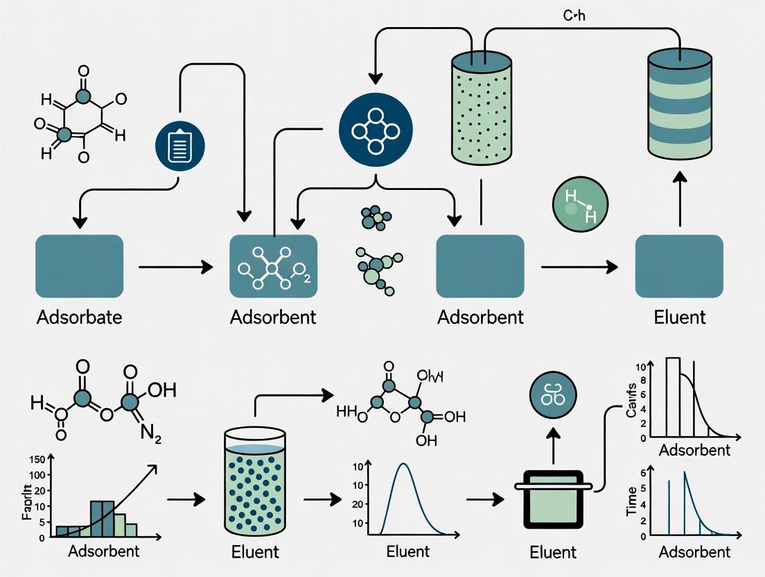
Diagrams

Title: Stages of Batch Adsorption Mechanism

Title: Standard Batch Adsorption Experimental Workflow

The Scientist's Toolkit: Key Research Reagent Solutions

Table 3: Essential Materials for Batch Adsorption Studies

Item	Function & Rationale
Model Adsorbate (e.g., Methylene Blue, Ibuprofen)	A well-characterized compound with reliable analytical detection, used for standardizing and comparing adsorbent performance.
Buffer Solutions (pH 2-10)	To control solution pH, a critical parameter affecting adsorbate speciation, adsorbent surface charge, and thus adsorption efficiency.
High-Purity Solvents (HPLC-grade Water, Methanol)	To prepare stock and standard solutions without introducing interfering contaminants that could skew capacity results.
Background Electrolyte (e.g., 0.01M NaCl)	To maintain constant ionic strength, mimicking real conditions and screening electrostatic interactions.
Desorbing Agent (e.g., 0.1M NaOH, 80% Ethanol)	To study adsorbent regeneration by reversing the adsorption process, critical for economic feasibility studies.
Certified Reference Materials (CRMs)	For accurate calibration of analytical instruments (HPLC, ICP-MS) to ensure precise and accurate concentration measurements.

Adsorbent vs. Adsorbate, Capacity, Equilibrium, and Kinetics

Within the methodological framework of a thesis on batch adsorption studies, precise definition of core terms is critical. This protocol details their application in pharmaceutical and environmental research.

• Adsorbent: The solid, porous material (e.g., activated carbon, silica gel, resin) that provides the surface for molecular attachment.
• Adsorbate: The dissolved substance (e.g., drug impurity, pollutant, protein) that becomes attached to the adsorbent's surface from the fluid phase.
• Capacity: The maximum amount of adsorbate that can be retained per unit mass of adsorbent under specified conditions, typically expressed as q_e (mg/g).
• Equilibrium: The state where the rate of adsorbate molecules attaching to the adsorbent equals the rate detaching, resulting in no net change in solution concentration.
• Kinetics: The study of the rate of the adsorption process and the factors influencing the time required to reach equilibrium.

Application Notes: Data Interpretation & Modeling

Recent studies emphasize integrating equilibrium and kinetic analysis for scalable process design. Key quantitative models are summarized below.

Table 1: Common Adsorption Isotherm Models (Equilibrium)

Model Name	Equation	Linear Form	Key Parameters	Applicability
Langmuir	qe = (qmax KL Ce) / (1 + KL Ce)	Ce/qe = 1/(KLqmax) + Ce/qmax	qmax (mg/g), KL (L/mg)	Monolayer adsorption on homogeneous sites.
Freundlich	qe = KF Ce1/n	log qe = log KF + (1/n) log Ce	KF, n (heterogeneity factor)	Empirical; multilayer adsorption on heterogeneous surfaces.
Temkin	qe = (RT/bT) ln(KT Ce)	qe = B1 ln KT + B1 ln Ce	KT (L/g), B1	Accounts for adsorbent-adsorbate interactions; heat of adsorption decreases linearly with coverage.

Table 2: Common Adsorption Kinetic Models

Model Name	Equation	Linear Form	Parameters	Insight Provided
Pseudo-First-Order (PFO)	dqt/dt = k1(qe - qt)	log(qe - qt) = log(qe) - (k1/2.303)t	k1 (1/min)	Adsorption rate proportional to available sites. Often fails to fit full range.
Pseudo-Second-Order (PSO)	dqt/dt = k2(qe - qt)2	t/qt = 1/(k2qe2) + t/qe	k2 (g/mg·min)	Rate depends on square of available sites; often describes chemisorption.
Intraparticle Diffusion	qt = kid t1/2 + C	qt = kid t1/2 + C	kid (mg/g·min1/2), C	Multi-linear plot identifies if pore diffusion is the rate-limiting step.

Batch Adsorption Study Methodology Workflow

Experimental Protocols

Protocol 1: Determination of Adsorption Kinetics

Objective: To determine the rate of adsorbate uptake and the time to reach equilibrium.

• Preparation: Dry and accurately weigh a fixed mass (e.g., 0.10 g ± 0.001 g) of adsorbent into multiple 150 mL Erlenmeyer flasks.
• Adsorbate Solution: Prepare a stock solution of the target adsorbate (e.g., 1000 mg/L) in appropriate buffer or solvent. Dilute to the desired initial concentration (C₀, e.g., 100 mg/L).
• Initiation: Add 100 mL of adsorbate solution to each flask. Cap and place on a temperature-controlled orbital shaker.
• Sampling: Remove flasks at predetermined time intervals (e.g., 5, 15, 30, 60, 120, 240, 480 min).
• Separation: Immediately filter each sample through a 0.45 µm membrane filter to separate the adsorbent.
• Analysis: Quantify the residual adsorbate concentration (C_t) in the filtrate using calibrated analytical methods (HPLC, UV-Vis, etc.).
• Calculation: Compute the amount adsorbed at time t: q_t = ( (C₀ - C_t) * V ) / m, where V is volume (L) and m is adsorbent mass (g).
• Modeling: Plot q_t vs. time. Fit data to kinetic models (Table 2) using non-linear regression.

Protocol 2: Determination of Adsorption Isotherm & Capacity

Objective: To determine the equilibrium adsorption capacity at a constant temperature.

• Preparation: Weigh identical masses of adsorbent into a series of 8-12 flasks.
• Concentration Series: To each flask, add equal volumes of adsorbate solution, varying C₀ across a broad range (e.g., 10-500 mg/L). Include a blank (adsorbent + solvent).
• Equilibration: Shake flasks at constant temperature until equilibrium is confirmed (e.g., 24 hrs, based on kinetic data).
• Separation & Analysis: Filter and analyze the equilibrium concentration (C_e) as in Protocol 1.
• Calculation: Compute the equilibrium capacity: q_e = ( (C₀ - C_e) * V ) / m.
• Modeling: Plot q_e vs. C_e. Fit data to isotherm models (Table 1). The parameter q_max from the best-fit model represents the theoretical maximum capacity.

Proposed Sequential Mass Transfer Pathway in Adsorption

The Scientist's Toolkit

Table 3: Essential Research Reagent Solutions & Materials

Item	Function & Rationale
Model Adsorbates (e.g., Methylene Blue, Phenol, BSA)	Standardized compounds with reliable analytical detection methods for benchmarking adsorbent performance.
Activated Carbon (Powdered/Granular)	High-surface-area reference adsorbent for comparative studies of organic contaminant removal.
Ion-Exchange Resins (Cationic/Anionic)	Functionalized polymers for studying charged adsorbate (e.g., metal ions, charged drug molecules) interactions.
Mesoporous Silica (e.g., SBA-15, MCM-41)	Tunable, well-defined pore geometry adsorbent for studying size-exclusion and surface modification effects.
Phosphate Buffered Saline (PBS), pH 7.4	Maintains physiological pH and ionic strength for adsorption studies relevant to biopharmaceuticals.
0.45 µm Nylon Membrane Filters	Ensures complete removal of adsorbent fines for accurate residual concentration measurement without interference.
Temperature-Controlled Orbital Shaker	Provides consistent mixing and temperature, critical for reproducible kinetic and equilibrium data.
Analytical Balance (±0.1 mg)	Precise weighing of adsorbent mass is essential for accurate calculation of qe and qt.

The Role of Batch Adsorption in Modern Drug Development and Bioprocessing

Batch adsorption is a fundamental unit operation in downstream bioprocessing, enabling the selective capture and purification of target molecules like monoclonal antibodies (mAbs), vaccines, and gene therapy vectors. Within a broader thesis on batch adsorption methodology, this process serves as a critical experimental platform for rapid adsorbent screening, binding isotherm determination, and preliminary process parameter optimization before scaled-up column chromatography.

Application Notes

Note 1: Primary Capture of Monoclonal Antibodies Batch adsorption is routinely employed for the initial capture of mAbs from clarified cell culture supernatant using Protein A-functionalized adsorbents. It allows for the rapid assessment of dynamic binding capacity under different conditions (pH, conductivity). Recent studies indicate modern alkali-stable Protein A ligands achieve equilibrium binding capacities of >50 mg/mL in batch contact studies, facilitating high-titer process development.

Note 2: Endotoxin and Impurity Removal In plasmid DNA (pDNA) and viral vector purification, batch adsorption with selective adsorbents like anion-exchange particles or activated charcoal is key for removing host cell impurities. Data shows multi-modal adsorbents can reduce endotoxin levels by >99% while maintaining pDNA recoveries above 85%.

Note 3: Continuous Bioprocessing Integration Batch adsorption in a stirred-tank format is a cornerstone of continuous downstream processing. It functions as a capture "pod" or a side-stream impurity trap. Current industry data demonstrates its use can reduce resin volume requirements by 20-30% compared to traditional fixed-bed columns for certain capture steps.

Table 1: Batch Adsorption Performance for Selected Biologics

Target Molecule	Adsorbent Type	Key Binding Condition (pH)	Max. Equilibrium Capacity (mg/mL)	Key Impurity Removed	Reduction (%)
mAb (IgG1)	Protein A Agarose	7.4	55.2	HCP	98.5
Plasmid DNA	Anion-Exchange Silica	8.0	4.1 (mg pDNA/mL)	Endotoxin	99.8
mRNA	Oligo-dT Cellulose	7.5	2.8 (mg mRNA/mL)	dsRNA, IVT reagents	95.0
Viral Vector (AAV)	Affinity Core Shell	8.2	1.5e13 (vg/mL)	Empty Capsids	70.0

Table 2: Impact of Critical Process Parameters on mAb Batch Adsorption

Parameter	Tested Range	Optimal Value (for Protein A)	Effect on Dynamic Binding Capacity
pH	6.0 - 8.5	7.2 - 7.6	±15% variation across range
Conductivity	1 - 20 mS/cm	5 - 10 mS/cm	>20% loss at high end
Contact Time	5 - 120 min	30 - 60 min	<5% gain after 60 min
Adsorbent Loading	5 - 20% v/v	10% v/v	Linear increase to 10%, plateau beyond

Experimental Protocols

Protocol 1: Determining Binding Isotherm for a mAb

Objective: To generate a Langmuir adsorption isotherm for a mAb on a novel adsorbent. Materials: Clarified harvest, adsorbent slurry, binding buffer (50 mM Tris, 150 mM NaCl, pH 7.4), tubes.

• Equilibration: Aliquot 1 mL of adsorbent slurry into 10 separate 15-mL conical tubes. Wash 3x with 10 mL binding buffer.
• Loading: Prepare 10 different mAb solutions in binding buffer (e.g., 0.1 to 10 mg/mL). Add 10 mL of each solution to a tube. Seal and mix on a rotary shaker for 60 min at 25°C.
• Separation: Centrifuge tubes at 500 x g for 5 min. Collect supernatant.
• Analysis: Measure residual mAb concentration in supernatant via UV absorbance at 280 nm.
• Calculation: Calculate adsorbed mAb per unit volume adsorbent (Q) = (Cinitial - Cfinal) * Volume / Adsorbent Volume. Plot Q vs. C_final.

Protocol 2: High-Throughput Screening of Adsorbents

Objective: Screen 96 different adsorbent/condition combinations for impurity removal. Materials: 96-well filter plate with adsorbents, microplate shaker, vacuum manifold, analytics plate reader.

• Plate Preparation: Dispense 50 µL of settled adsorbent into each well of a 96-well filter plate.
• Equilibration: Add 200 µL of appropriate buffer to each well. Apply vacuum to drain. Repeat twice.
• Batch Binding: Add 150 µL of clarified feedstock (pre-adjusted to test pH/conductivity) to each well. Seal plate and agitate on microplate shaker for 45 min.
• Filtration: Apply vacuum to collect flow-through into a collection plate.
• Analysis: Use HPLC or plate-based assays (e.g., for HCP, DNA) to analyze each flow-through for target purity and yield.

Visualizations

Title: Batch Adsorption Basic Workflow

Title: Methodology Links to Applications

The Scientist's Toolkit: Key Research Reagent Solutions

Item	Function in Batch Adsorption Studies
Functionalized Agarose/Cellulose Beads	Base matrix for ligand immobilization; provides hydrophilic, porous support for biomolecule binding.
Protein A/G/L Affinity Ligands	Recombinant or native proteins for high-affinity, selective capture of antibody classes and fragments.
Anion/Cation Exchange Particles	Charged surfaces (DEAE, Q, CM, SP) for binding based on target molecule's net charge at specific pH.
Multi-Modal or Mixed-Mode Adsorbents	Combine multiple interactions (e.g., hydrophobic, ionic) for challenging separations like impurity removal.
Magnetic Responsive Adsorbents	Particles with magnetic cores for rapid separation in high-throughput screening applications.
Equilibration/Binding Buffers	Define pH and ionic strength to modulate adsorption selectivity and capacity.
Microplate-Based Filter Plates	Enable parallel, small-volume batch adsorption experiments for high-throughput screening.
Host Cell Protein (HCP) ELISA Kit	Critical analytical tool for quantifying impurity clearance efficiency.
DNA-Binding Fluorescent Dye (e.g., PicoGreen)	Sensitive detection of residual nucleic acid impurities in flow-through.

Batch adsorption studies are a foundational methodology in biochemical engineering and pharmaceutical research, providing critical data on equilibrium, kinetics, and capacity for diverse sorbent-ligand systems. This application note, framed within a broader thesis on optimizing batch adsorption protocols, details specific methodologies for three pivotal applications: medical toxin removal, monoclonal antibody (mAb) purification, and targeted drug delivery system development. The principles of static binding capacity (SBC), adsorption isotherms (Langmuir, Freundlich), and kinetic models (pseudo-first/second order) underpin the experimental design across these domains.

Application Notes & Protocols

Toxin Removal: Heparin for LPS Detoxification

Objective: To determine the adsorption capacity of immobilized heparin for bacterial lipopolysaccharide (LPS) endotoxin in a simulated serum solution. Background: Endotoxin removal is critical in sepsis treatment and biopharmaceutical safety. Heparin, a sulfated glycosaminoglycan, binds to the Lipid A moiety of LPS via electrostatic interactions.

Protocol:

• Sorbent Preparation: Covalently immobilize heparin (from porcine intestinal mucosa) onto cross-linked agarose beads (e.g., Sepharose 4B) using cyanogen bromide (CNBr) activation. Wash extensively with endotoxin-free water and store in 20% ethanol at 4°C.
• Toxin Solution: Prepare LPS (E. coli O55:B5) spiked solutions in sterile, endotoxin-free phosphate-buffered saline (PBS) with 0.1% bovine serum albumin (BSA) at concentrations of 10, 50, 100, 500, and 1000 EU/mL.
• Batch Adsorption: In sterile polypropylene tubes, add 100 µL of heparin-bead slurry (settled volume) to 1 mL of each LPS solution. Run in triplicate. Include controls (beads without heparin, solution without beads).
• Incubation: Rotate tubes end-over-end at 25°C for 2 hours (determined from kinetic studies to reach equilibrium).
• Separation & Analysis: Centrifuge at 500 x g for 2 minutes. Collect supernatant. Quantify residual LPS using a chromogenic Limulus Amebocyte Lysate (LAL) assay. Calculate adsorbed LPS per mL of sorbent.
• Data Modeling: Fit equilibrium data to Langmuir isotherm: q_e = (q_max * C_e) / (K_d + C_e), where q_e is amount adsorbed, C_e is equilibrium concentration, q_max is maximum capacity, and K_d is dissociation constant.

Table 1: Batch Adsorption Data for Heparin vs. LPS

Initial LPS (EU/mL)	Equilibrium LPS, C_e (EU/mL)	Adsorbed LPS, q_e (EU/mL gel)	Removal Efficiency (%)
10	0.5 ± 0.1	95 ± 1	95.0
50	4.2 ± 0.5	458 ± 5	91.6
100	12.1 ± 1.2	879 ± 12	87.9
500	85.0 ± 8.3	4150 ± 83	83.0
1000	210 ± 15	7900 ± 150	79.0

Langmuir Fit: q_max = 8500 ± 200 EU/mL gel, K_d = 45 ± 5 EU/mL, R² = 0.994.

Antibody Purification: Protein A Affinity Chromatography

Objective: To establish a batch binding protocol for capturing human IgG from clarified cell culture supernatant using Protein A agarose, prior to column chromatography. Background: Protein A binds the Fc region of antibodies with high specificity and affinity (~10 nM K_d), enabling single-step purification.

Protocol:

• Resin Equilibration: Suspend high-performance Protein A agarose resin (e.g., MabSelect) and wash with 5 column volumes (CV) of equilibration buffer (25 mM Tris, 150 mM NaCl, pH 7.4).
• Sample Preparation: Clarify Chinese Hamster Ovary (CHO) cell supernatant containing mAb by centrifugation (10,000 x g, 20 min) and 0.22 µm filtration. Adjust pH to 7.4 if necessary.
• Batch Binding: Combine 1 mL of settled resin with 10 mL of clarified supernatant in a 50 mL conical tube. Final mAb concentration should be ≤ 10 mg/mL resin to avoid overload.
• Binding & Washing: Mix gently on a rotator for 1 hour at 4-25°C. Allow resin to settle, then aspirate supernatant. Wash resin with 10 CV of equilibration buffer, followed by 5 CV of a stringent wash (25 mM Tris, 500 mM NaCl, pH 7.4).
• Elution Testing: Perform small-scale batch elutions. Add 1 CV of various elution buffers (e.g., 100 mM Glycine-HCl, pH 3.0; 100 mM Citrate, pH 3.5) to aliquots of washed resin. Mix for 5 minutes, neutralize immediately with 1 M Tris, pH 9.0. Analyze by SDS-PAGE and UV A280.
• Capacity Calculation: Determine dynamic binding capacity (DBC) by frontal analysis or static capacity by depletion.

Table 2: Performance Metrics for Protein A Batch Capture

Parameter	Value
Resin Binding Capacity (Theoretical)	≥ 50 mg human IgG/mL resin
Typical Binding Yield (Batch)	95-99%
Optimal Binding pH	7.0 - 7.4
Optimal Elution pH	2.5 - 3.5 (Glycine or Citrate)
Common Impurity Reduction	Host Cell Protein (HCP) > 95%, DNA > 99%

Drug Delivery: Mesoporous Silica Nanoparticle (MSN) Loading

Objective: To load an anti-cancer drug (e.g., Doxorubicin) into amine-functionalized MSNs and characterize the adsorption isotherm. Background: MSNs offer high surface area (>1000 m²/g) and tunable pores for drug encapsulation. Surface functionalization modulates loading and release.

Protocol:

• Nanoparticle Synthesis & Functionalization: Synthesize MSNs via sol-gel (CTAB template) method. Functionalize with (3-aminopropyl)triethoxysilane (APTES) to yield amine-MSNs. Characterize size (DLS, TEM), zeta potential, and surface area (BET).
• Drug Solution: Prepare doxorubicin HCl (DOX) solutions in PBS (pH 7.4) at concentrations from 0.05 to 2.0 mg/mL.
• Loading Study: Disperse 1 mg of amine-MSNs into 1 mL of each DOX solution. Protect from light. Vortex and incubate under constant shaking (200 rpm) at 37°C for 24 hours.
• Separation & Quantification: Pellet nanoparticles by ultracentrifugation (15,000 rpm, 20 min). Measure absorbance of supernatant at 480 nm. Calculate loaded drug: Loading Capacity (wt%) = (Mass of drug loaded / Mass of NPs) * 100.
• Release Kinetics: Re-suspend loaded NPs in PBS (pH 7.4 and pH 5.0, simulating endosomal conditions). Place in dialysis bag (MWCO 12-14 kDa). Sample external buffer at intervals, measure DOX fluorescence (Ex/Em: 480/590 nm).
• Modeling: Fit adsorption data to Freundlich isotherm (q_e = K_F * C_e^(1/n)) to describe heterogeneous surface binding.

Table 3: Doxorubicin Loading & Release from Amine-MSNs

Initial DOX Conc. (mg/mL)	Loading Capacity (wt%)	Encapsulation Efficiency (%)	BET Surface Area (m²/g)
0.05	4.1 ± 0.3	82.0	1050 ± 50
0.2	14.5 ± 1.1	72.5	1050 ± 50
0.5	28.0 ± 2.0	56.0	1050 ± 50
1.0	38.2 ± 2.5	38.2	1050 ± 50
2.0	45.0 ± 3.0	22.5	1050 ± 50

Freundlich Fit: K_F = 18.2, n = 1.76, R² = 0.985. Cumulative Release at 24h: pH 7.4 = 25±3%, pH 5.0 = 65±5%.

Visualizations

Diagram 1: LPS Removal Batch Workflow

Diagram 2: mAb Purification Batch Process

Diagram 3: Nanoparticle Drug Loading & Release

The Scientist's Toolkit: Key Reagent Solutions

Table 4: Essential Research Materials for Batch Adsorption Studies

Item/Reagent	Primary Function & Application Context
Activated Chromatography Resins (e.g., CNBr-Activated Sepharose)	Immobilization of ligands (heparin, antibodies) for affinity adsorption studies.
Limulus Amebocyte Lysate (LAL) Assay Kits	Quantitative, sensitive detection and quantification of bacterial endotoxins (LPS) in solutions.
Recombinant Protein A/G/L Resins	High-affinity capture of antibodies from serum, hybridoma, or cell culture sources for purification.
Functionalized Mesoporous Silica Nanoparticles	High-surface-area platform for studying adsorption and controlled release of drug molecules.
Chromatography Buffers (Equilibration, Binding, Elution)	Maintain optimal pH and ionic strength for specific adsorption and desorption of target biomolecules.
Dynamic Light Scattering (DLS) & Zeta Potential Analyzer	Characterize nanoparticle size, size distribution, and surface charge before/after functionalization.
MicroBCA or Bradford Protein Assay Kits	Rapid, colorimetric quantification of protein concentrations in supernatants and eluates.

This document presents a series of application notes and standardized protocols for investigating critical operational parameters in batch adsorption studies. The work is framed within a broader thesis aimed at developing a rigorous, reproducible, and predictive methodology for adsorption research, with applications spanning contaminant removal, drug delivery system development, and bioseparation processes. Systematic evaluation of pH, temperature, ionic strength, and initial adsorbate concentration is fundamental to elucidating adsorption mechanisms, optimizing capacity, and enabling process scale-up.

Table 1: Summary of Critical Factors and Their Typical Effects on Adsorption Processes

Factor	Typical Experimental Range	Primary Influence	Key Measurable Outcomes
pH	2.0 - 10.0	Surface charge of adsorbent, ionization state of adsorbate, speciation.	Zeta potential, adsorption capacity (qe), point of zero charge (PZC).
Temperature	20°C - 60°C	Kinetic energy, thermodynamic feasibility, adsorbent stability.	Adsorption capacity (qe), rate constants (k), ΔG°, ΔH°, ΔS°.
Ionic Strength	0.001 - 1.0 M NaCl/KNO3	Electrical double layer compression, competitive binding, "salting-out".	Adsorption capacity (qe), distribution coefficient (Kd).
Concentration	Variable (e.g., 10-500 mg/L)	Driving force for mass transfer, active site saturation.	qe, adsorption isotherm fit (Langmuir, Freundlich), maximum capacity (qmax).

Table 2: Example Data from a Model Study on Pharmaceutical Adsorption

Condition	pH	Temp (°C)	Ionic Strength (M)	qe (mg/g)	Removal (%)	Proposed Dominant Mechanism
Optimal	6.0	25	0.01	98.5	98.5	Electrostatic attraction, π-π interaction
Acidic	3.0	25	0.01	22.1	22.1	Repulsion/Competition with H⁺
High Salt	6.0	25	0.5	65.3	65.3	Double-layer compression
Elevated Temp	6.0	45	0.01	112.3	95.0*	Endothermic chemisorption

*Note: *Lower % removal at higher qe is due to increased solubility/desorption at higher temperature; calculation based on initial concentration.

Experimental Protocols

Protocol 3.1: Systematic Batch Adsorption Study for Parameter Optimization

Objective: To determine the individual and interactive effects of pH, temperature, ionic strength, and initial concentration on adsorption capacity and kinetics.

Materials: See "Scientist's Toolkit" (Section 5). Procedure:

• Adsorbent Preparation: Precisely weigh (e.g., 10.0 ± 0.1 mg) of adsorbent into a series of clean, dry serum vials or centrifuge tubes.
• Solution Conditioning:
  • pH Variation: Prepare adsorbate stock solution. Adjust pH of aliquots from 2 to 10 using 0.1M HCl or NaOH. Measure final pH after adjustment.
  • Ionic Strength Variation: Add calculated volumes of NaCl or KNO3 stock to achieve desired ionic strength (0.001M to 0.5M).
  • Concentration Variation: Dilute stock to desired initial concentrations (e.g., 10, 50, 100, 200 mg/L).
• Initiation of Experiment: Add a fixed volume (e.g., 10 mL) of the conditioned adsorbate solution to each adsorbent-containing vial. Seal immediately.
• Temperature Control: Place vials in temperature-controlled shaker incubators set at desired temperatures (e.g., 25°C, 35°C, 45°C).
• Kinetic Sampling: Agitate at constant speed (e.g., 150 rpm). For kinetic profiles, remove duplicate vials at predetermined time intervals (e.g., 5, 15, 30, 60, 120, 240 min).
• Separation: Centrifuge samples immediately (e.g., 4000 rpm for 10 min) or filter through a 0.45 μm membrane.
• Analysis: Quantify residual adsorbate concentration in supernatant/filtrate using calibrated HPLC-UV, spectrophotometry, or other appropriate analytical methods.
• Data Calculation: Calculate adsorption capacity at time t, qt (mg/g), and at equilibrium, qe (mg/g): qt or qe = (C0 - Ct or Ce) * V / m, where C0, Ct, Ce are initial, at time t, and equilibrium concentrations (mg/L), V is solution volume (L), and m is adsorbent mass (g).

Protocol 3.2: Determination of Point of Zero Charge (PZC) Objective: To identify the pH at which the adsorbent surface has a net neutral charge.

• Prepare 50 mL of 0.01M NaCl in a series of 10 Erlenmeyer flasks.
• Adjust initial pH (pHi) from 2 to 10 using 0.1M HCl/NaOH.
• Add a fixed mass of adsorbent (e.g., 0.1 g) to each flask. Cap and agitate for 24-48 h.
• Measure final pH (pHf). Plot ΔpH (pHf - pHi) vs. pHi. The point where ΔpH = 0 is the PZC.

Visualization of Methodology and Relationships

Title: Adsorption Parameter Study Workflow

Title: Factor-Property-Effect-Outcome Logic Chain

The Scientist's Toolkit

Table 3: Key Research Reagent Solutions and Essential Materials

Item / Solution	Specification / Preparation	Primary Function in Experiments
Adsorbent	e.g., Activated carbon, polymeric resin, MOF, hydrogel. Milled and sieved to specific particle size (e.g., 75-150 μm).	The solid substrate whose surface properties are being characterized for uptake of target molecules.
Adsorbate Stock Solution	High-purity compound dissolved in appropriate solvent (often water, buffer, or simulant). Stored at 4°C in the dark.	Provides the standardized target molecule for adsorption studies.
pH Adjustment Solutions	0.1M HCl and 0.1M NaOH, prepared from concentrated stocks using CO2-free deionized water.	Precisely modulates solution pH to study its profound effect on adsorption mechanisms.
Ionic Strength Modifier	1.0M NaCl or KNO3 (ACS grade) solution. KNO3 is preferred for spectroscopic analysis to avoid Cl⁻ interference.	Controls the ionic environment to study electrostatic interactions and competition.
Background Electrolyte	0.01M NaCl or NaNO3. Used as a constant baseline ionic medium in all experiments unless varying IS.	Maintains a constant ionic strength, minimizing uncontrolled variations in double-layer thickness.
Phosphate or Britton-Robinson Buffer	Use with caution at low concentrations (e.g., ≤0.01M) only if necessary, as buffer ions may compete for adsorption sites.	Maintains constant pH in studies where pH control is critical and adsorption is weak.
Centrifuge Tubes / Serum Vials	Polypropylene, chemically resistant, with secure caps (e.g., 15-50 mL capacity).	Reaction vessels for batch experiments; must be non-adsorbing to the contaminant.
0.45 μm Nylon Membrane Filters	Syringe-driven, sterile if needed. Pre-rinse with sample to avoid saturation effects.	Separation of adsorbent from solution for accurate residual concentration analysis.

Within the methodology of batch adsorption studies, the selection of an appropriate adsorbent is critical. This section provides a comparative overview of common adsorbent classes, detailing their properties to inform experimental design for researchers in pharmaceuticals and environmental science.

Table 1: Core Properties of Common Adsorbent Classes

Adsorbent Class	Typical Surface Area (m²/g)	Primary Pore Size Range	Common Functional Groups	pH Stability Range	Thermal Stability (°C)
Activated Carbon	500 - 1500	Micropores (<2 nm)	Carboxyl, Phenolic, Carbonyl	2 - 11	< 300 (inert atm)
Polymeric Resins (e.g., Styrene-DVB)	400 - 800	Mesopores (2-50 nm)	Sulfonic acid, Amine, Phenyl	0 - 14	< 150
Natural Polymers (e.g., Chitosan)	Low - Moderate	Macropores (>50 nm)	Amino, Hydroxyl	4 - 8	< 200
Synthetic Polymers (e.g., Imprinted)	50 - 600	Tunable Meso/Macro	Custom (e.g., Vinyl, Acrylate)	2 - 12	Varies by polymer
Novel Materials (e.g., MOFs)	1000 - 7000	Micropores, Tunable	Metal ions, Organic linkers	3 - 11 (varies)	150 - 400
Silica-based	200 - 1000	Mesopores (2-50 nm)	Silanol, Modified (e.g., C18)	2 - 8	< 600

Application Notes for Batch Adsorption Studies

Activated Carbon

• Primary Applications: Removal of organic contaminants (dyes, pharmaceuticals, endotoxins), decolorization, VOC capture in drug manufacturing.
• Key Considerations: Surface chemistry is highly dependent on precursor (wood, coconut shell, coal) and activation method (steam, chemical). Oxygen-containing groups influence adsorption of polar compounds. May require pre-washing to remove fines and neutralize pH.
• Protocol - Pre-treatment: Weigh 1.0 g of powdered activated carbon. Add to 100 mL of 0.1M HCl. Stir for 1 hour. Filter and wash with deionized water until filtrate pH is neutral. Dry at 110°C for 12 hours. Store in a desiccator.

Polymeric & Ion-Exchange Resins

• Primary Applications: Purification of antibiotics, separation of biomolecules, metal ion recovery from catalyst streams, decaffeination.
• Key Considerations: Selection is based on matrix (polar/non-polar), particle size, and functional group (cationic/anionic). Swelling behavior in different solvents must be accounted for in volume-based studies.
• Protocol - Capacity Determination (Cation Exchange Resin): 1) Pre-treat 1.0 g wet resin with 50 mL of 1M NaCl for 30 min to convert to Na⁺ form. Rinse. 2) Add 50 mL of 0.1M HCl solution. Stir for 2 hours. 3) Titrate the supernatant against 0.1M NaOH to determine H⁺ uptake.

Natural and Synthetic Polymers

• Primary Applications: Chitosan for heavy metal and dye removal; Molecularly Imprinted Polymers (MIPs) for selective extraction of drug enantiomers or specific contaminants.
• Key Considerations: Biopolymers like chitosan require acidic conditions for solubility. MIPs offer high selectivity but synthesis (template, monomer, cross-linker ratio) is complex and requires rigorous template removal validation.

Novel Materials (MOFs, COFs, Graphene Oxides)

• Primary Applications: High-capacity storage (H₂, CO₂), targeted drug delivery, selective adsorption of strategic metals, advanced catalytic supports.
• Key Considerations: Exceptional surface area and tunability. Stability (hydrolytic, thermal) can be a constraint. Cost and scalability for large-scale batch studies may be prohibitive.
• Protocol - Activation of MOFs: To remove solvent from pores, place synthesized MOF (e.g., MIL-101(Cr)) in a Schlenk tube. Apply dynamic vacuum (<0.1 mbar) while heating to 150°C (or temperature below framework decomposition) for 12 hours. Cool under vacuum before sealing.

Table 2: Quantitative Adsorption Performance Benchmarks

Adsorbent (Example)	Target Adsorbate	Typical qmax (mg/g)	Approx. Equilibrium Time (hrs)	Optimal pH	Key Binding Mechanism
Activated Carbon (F400)	Methylene Blue	250 - 300	2 - 4	7 - 9	π-π interactions, Electrostatic
Cationic Resin (Amberlite IR120)	Cu²⁺	45 - 55	1 - 2	5 - 6	Ion Exchange
Chitosan Beads	Cr(VI)	100 - 150	3 - 5	3 - 4	Electrostatic, Chelation
MIP (Theophylline)	Theophylline	8 - 12	1	6.5 - 7.5	Shape-specific Hydrogen Bonding
MOF (ZIF-8)	CO₂	40 - 55 (at 1 bar)	< 0.5	N/A	Physisorption in Pores
Graphene Oxide	Pb²⁺	400 - 500	1 - 2	5 - 6	Complexation with O groups

Standardized Batch Adsorption Experiment Protocol

This protocol provides a generalizable methodology for evaluating any adsorbent within a thesis on batch adsorption studies.

Aim: To determine the adsorption capacity and kinetics of a target compound on a selected adsorbent.

Materials: Adsorbent, adsorbate stock solution, buffer solutions, orbital shaker incubator, centrifuge, analytical instrument (HPLC, UV-Vis, AAS), 50 mL conical centrifuge tubes.

Procedure:

• Adsorbent Preparation: Sieve adsorbent to desired particle size range (e.g., 100-200 µm). Pre-treat/activate as per material requirements (see Section 2 protocols). Dry to constant weight.
• Solution Preparation: Prepare a precise stock solution of the target adsorbate. Prepare buffer to maintain constant ionic strength and pH.
• Batch Equilibrium Study (Isotherm):
  • Prepare a series of 8-10 centrifuge tubes.
  • Add a fixed mass (e.g., 10.0 ± 0.1 mg) of adsorbent to each tube.
  • Add varying volumes of stock to each tube to create a concentration gradient (e.g., 10-500 mg/L). Fill each tube to 25 mL with buffer.
  • Seal tubes and agitate in a shaker incubator at constant speed (e.g., 150 rpm) and temperature (e.g., 25°C) for 24 hours (or predetermined equilibrium time).
  • Centrifuge tubes at 4000 rpm for 10 min. Filter supernatant (0.45 µm syringe filter).
  • Analyze filtrate concentration (C_e).
  • Calculate adsorption capacity: q_e = (C₀ - C_e) * V / m.
• Batch Kinetic Study:
  • Set up multiple tubes with identical adsorbent dose and initial adsorbate concentration.
  • Agitate as above. Remove tubes at predetermined time intervals (e.g., 5, 15, 30 min, 1, 2, 4, 8, 24 hrs).
  • Process and analyze each tube as in Step 3.
  • Plot q_t vs. time.

Visualization of Methodologies

Title: Batch Adsorption Study Workflow

Title: Adsorption Mass Transfer Pathway

The Scientist's Toolkit: Essential Research Reagents & Materials

Table 3: Key Reagents and Materials for Batch Adsorption Studies

Item	Function in Protocol	Example/Note
Model Adsorbate	The target compound for removal/study.	Methylene Blue (dye), Tetracycline (antibiotic), Cu(II) nitrate (heavy metal).
Buffer Salts (e.g., Phosphate, Acetate)	Maintain constant pH and ionic strength, critical for reproducibility.	0.01M phosphate buffer, pH 7.0.
High-Purity Solvents (HPLC grade Water, Methanol)	Prepare stock solutions, rinse adsorbents, dilute samples for analysis.	Ensure low UV absorbance for HPLC analysis.
Syringe Filters (0.45 µm, 0.22 µm)	Clarify supernatant post-centrifugation prior to instrumental analysis.	Nylon for aqueous, PTFE for organic solutions.
Certified Reference Standards	Calibrate analytical instruments for accurate concentration determination.	Crucial for quantifying adsorption capacity (q).
Centrifuge Tubes (Conical, polypropylene)	Container for individual batch experiments. Must be chemically inert.	50 mL tubes are standard for 25 mL batch volume.
Orbital Shaker Incubator	Provide constant agitation and temperature control during equilibration.	Ensures proper mixing and constant T (±0.5°C).
Analytical Balance (±0.1 mg)	Precisely weigh small masses of adsorbent and prepare stock solutions.	Foundational for all quantitative calculations.

Step-by-Step Protocol: Designing and Executing a Batch Adsorption Experiment

1. Introduction Within the methodology research for batch adsorption studies, the pre-experimental planning phase is foundational. This phase systematically translates a research question into a viable experimental strategy. For studies aiming to develop or optimize adsorption processes—such as contaminant removal or targeted drug carrier design—precise objective definition and judicious model system selection dictate the relevance, reproducibility, and scalability of all subsequent findings.

2. Defining Hierarchical Research Objectives Clear objectives align experimental design with the overarching thesis goal of methodological rigor. Objectives should be structured hierarchically.

Table 1: Hierarchy and Examples of Research Objectives in Batch Adsorption Methodology

Objective Level	Description	Example for a Study on Antibiotic Adsorption
Primary Objective	The central, broad goal of the research project.	To establish a standardized protocol for evaluating novel biochar materials in adsorbing fluoroquinolone antibiotics from aqueous solutions.
Secondary Objectives	Specific, measurable aims that support the primary objective.	1. To quantify the adsorption capacity (Qe) of three biochar types for ciprofloxacin at pH 7.2. To determine the optimal contact time to reach equilibrium for each adsorbent.3. To model the adsorption kinetics using pseudo-first and pseudo-second order models.
Methodological Objectives	Goals related to the refinement or validation of the experimental method itself.	1. To compare the reproducibility of results using orbital shakers vs. wrist-action shakers.2. To validate a UV-Vis analytical method for ciprofloxacin quantification in the presence of biochar leachates.

3. Selecting Model Systems: Adsorbates and Adsorbents The choice of model systems must reflect both scientific relevance and experimental controllability.

3.1. Model Adsorbate Selection Criteria

• Relevance: Environmental pollutant (e.g., heavy metal, dye, pharmaceutical) or target biomolecule (e.g., protein, toxin).
• Analytical Tractability: Must be quantifiable at relevant concentrations using available instrumentation (e.g., HPLC, UV-Vis, ICP-MS).
• Stability: Should remain chemically stable under experimental conditions (pH, temperature, light).
• Representativeness: Serves as a proxy for a broader class of compounds.

3.2. Model Adsorbent Selection Criteria

• Material Type: Activated carbon, ion-exchange resins, molecularly imprinted polymers, biochars, functionalized silica.
• Physicochemical Properties: Defined surface area, porosity, particle size distribution, point of zero charge (PZC), and surface functional groups.
• Pre-treatment: Requires standardized pre-experimental protocols (washing, drying, sieving).

Table 2: Exemplar Model Systems for Methodological Batch Adsorption Studies

Study Focus	Recommended Model Adsorbate	Key Properties	Recommended Model Adsorbent	Rationale for Selection
Kinetics/Isotherm Modeling	Methylene Blue (C16H18ClN3S)	Cationic dye, λmax ≈ 665 nm, high solubility.	Powdered Activated Carbon (PAC), e.g., Norit GS 0.5	Well-characterized, high surface area (> 500 m²/g), serves as a benchmark.
pH-Dependent Studies	Cadmium Ions (Cd²⁺)	Divalent cationic metal, toxic pollutant.	Commercial Ion-Exchange Resin (e.g., Amberlite IR120 Na⁺)	Clear ion-exchange mechanism, highly sensitive to solution pH.
Bio-adsorbent Screening	Ciprofloxacin (C17H18FN3O3)	Amphoteric fluoroquinolone antibiotic, λmax ≈ 275 nm.	Biochars from defined feedstocks (e.g., oak wood, rice husk)	Variable surface chemistry ideal for testing structure-function relationships.

4. Core Experimental Protocol: Standardized Batch Adsorption Experiment This protocol is designed to fulfill secondary objectives related to capacity and kinetics.

4.1. Materials & Pre-Experimental Preparation

• Adsorbent: Pre-dry at 105°C for 24h, sieve to select 100-200 μm fraction, store in desiccator.
• Adsorbate Stock Solution: Precisely dissolve compound in background electrolyte solution (e.g., 0.01M NaCl) to ensure constant ionic strength.
• pH Adjustment: Adjust solution pH using 0.1M HCl or NaOH. Allow system to equilibrate for 24h pre-adsorption, as pH can drift.

4.2. Step-by-Step Procedure

• Setup: Prepare a series of 50 mL centrifuge tubes (or Erlenmeyer flasks) in triplicate.
• Loading: To each tube, add a precise mass (e.g., 10.0 ± 0.1 mg) of adsorbent and 25.0 mL of adsorbate solution at known initial concentration (C₀).
• Control: Prepare "blank" tubes (adsorbent in background electrolyte only) and "standard" tubes (adsorbate solution only, no adsorbent).
• Agitation: Place all tubes in a temperature-controlled orbital shaker. Agitate at a constant speed (e.g., 150 rpm) for a predetermined time (t).
• Separation: At time t, remove tubes and immediately centrifuge (e.g., 4000 rpm, 10 min) or filter (0.45 μm membrane) to separate solid adsorbent.
• Analysis: Quantify the equilibrium concentration (C_e) of the adsorbate in the supernatant using a calibrated analytical method (e.g., UV-Vis spectrophotometry).
• Calculation: Calculate the adsorption capacity at time t, Q_t (mg/g), using: Q_t = (C₀ - C_t) * V / m, where V is solution volume (L) and m is adsorbent mass (g).

5. The Scientist's Toolkit: Key Research Reagent Solutions

Table 3: Essential Materials for Batch Adsorption Studies

Item	Function / Rationale
Background Electrolyte (e.g., 0.01M NaCl or KNO3)	Maintains constant ionic strength, which controls the thickness of the electrical double layer around adsorbent particles, ensuring reproducible conditions.
pH Buffer Solutions	Used with caution. While they control pH, buffer ions (e.g., phosphate) can themselves adsorb or interfere. Their use must be reported and justified.
High-Purity Analytical Standards	Essential for calibrating quantification equipment (HPLC, UV-Vis). Purity >98% ensures accurate C0 and Ce determination.
Certified Reference Adsorbent	A well-characterized material (e.g., NIST Standard Reference Material) used for inter-laboratory method validation and troubleshooting.
0.45 μm Nylon Membrane Filters	For rapid phase separation post-adsorption. Material must be checked for non-specific adsorption of the target analyte.

6. Visualizing the Pre-Experimental Planning Workflow

Title: Flowchart for Adsorption Study Planning

7. Visualizing Data Flow in a Batch Experiment

Title: Data Flow in Adsorption Capacity Calculation

Within the broader methodological research for batch adsorption studies—a cornerstone in pharmaceutical development for impurity removal, drug delivery system design, and API purification—the reliability of results is intrinsically linked to the precision and appropriateness of the materials and equipment employed. This protocol serves as a comprehensive checklist and application guide, ensuring methodological rigor from sample preparation through data acquisition.

The Scientist's Toolkit: Essential Research Reagent Solutions

The following table details critical consumables and reagents fundamental to standardized batch adsorption studies.

Table 1: Key Research Reagent Solutions for Batch Adsorption Studies

Item	Function & Importance
Model Adsorbate Solution	A solution of known concentration of the target compound (e.g., drug, dye, impurity). Purity must be certified (e.g., HPLC-grade) to ensure accurate isotherm modeling.
Adsorbent Material	The solid phase (e.g., activated carbon, polymeric resin, silica gel). Key parameters: particle size distribution, specific surface area (BET), and pre-treatment/activation protocol.
Buffer Solutions	Maintain constant pH, ionic strength, and simulate biological or process conditions. Critical for studying adsorption thermodynamics and kinetics.
Competitive Ion Solutions	Solutions containing ions (e.g., Na+, Ca2+, Cl-) to study selectivity and interference in multicomponent systems.
Desorbing Agents	Solutions (e.g., organic solvents, pH-extreme buffers) used in regeneration studies to evaluate adsorbent reusability.
Mobile Phase for HPLC/UPLC	High-purity solvents and modifiers for the accurate quantification of adsorbate concentration pre- and post-adsorption.

Experimental Protocols

Protocol 1: Standard Batch Adsorption Isotherm Experiment

Objective: To determine the equilibrium relationship between the amount of adsorbate bound to the adsorbent and its concentration in solution at constant temperature and pH.

Materials & Equipment Checklist:

• Thermostated Incubator Shaker (precision: ±0.5°C)
• Analytical Balance (precision: ±0.1 mg)
• pH Meter (calibrated)
• Centrifuge (or vacuum filtration setup with appropriate membranes)
• UV-Vis Spectrophotometer or HPLC/UPLC System
• Volumetric Flasks, Pipettes
• Polypropylene/glass conical tubes (e.g., 15-50 mL)

Procedure:

• Adsorbent Preparation: Weigh predetermined masses (e.g., 5, 10, 20 mg) of dried adsorbent into a series of labeled tubes.
• Solution Preparation: Prepare a stock solution of the adsorbate at a known, high concentration. Dilute to create a series of initial concentrations (C₀).
• pH Adjustment: Adjust the pH of all solutions to the target value using dilute NaOH or HCl. Record final pH.
• Initiation: To each tube containing adsorbent, add a fixed volume (e.g., 10 mL) of adsorbate solution. Cap tubes tightly.
• Equilibration: Place all tubes in the thermostated shaker. Agitate at a constant speed (e.g., 150 rpm) at the target temperature (e.g., 25°C, 37°C) for a predetermined time (confirmed by kinetic studies to be sufficient for equilibrium, often 24h).
• Separation: Centrifuge tubes (or filter) to achieve solid-liquid separation.
• Analysis: Quantify the equilibrium concentration (Cₑ) in the supernatant/filtrate using calibrated analytical methods (e.g., UV-Vis at λmax, HPLC).
• Calculation: Calculate the equilibrium adsorption capacity, qₑ (mg/g): qₑ = (C₀ - Cₑ) * V / m, where V is solution volume (L) and m is adsorbent mass (g).

Protocol 2: Batch Adsorption Kinetic Study

Objective: To investigate the rate of adsorption and identify potential rate-controlling mechanisms.

Materials & Equipment Checklist: (Includes all from Protocol 1, with emphasis on)

• Multi-point/Time-Point Shaker or ability to remove samples sequentially.
• Micro-sampling equipment.

Procedure:

• Setup: Prepare a single, large-volume batch in a sealed vessel with known adsorbent dose and initial adsorbate concentration under controlled pH and temperature.
• Sampling: At predetermined time intervals (e.g., 1, 2, 5, 10, 20, 40, 60, 120 min), withdraw small, equal aliquots of the suspension.
• Immediate Separation: Rapidly filter or centrifuge each aliquot.
• Analysis: Measure the adsorbate concentration (Cₜ) in each sample.
• Calculation: Calculate the capacity at time t, qₜ (mg/g): qₜ = (C₀ - Cₜ) * V / m. Plot qₜ vs. time to generate the kinetic profile.

Data Presentation

Table 2: Example Equilibrium Isotherm Data for Methylene Blue on Activated Carbon (25°C, pH 7)

C₀ (mg/L)	Cₑ (mg/L)	Adsorbent Mass (mg)	qₑ (mg/g)	Removal Efficiency (%)
10.0	1.2	10.0	8.80	88.0
20.0	3.1	10.0	16.90	84.5
40.0	8.5	10.0	31.50	78.8
60.0	16.2	10.0	43.80	73.0
80.0	26.4	10.0	53.60	67.0

Table 3: Example Kinetic Data for Paracetamol Adsorption on Polymer Resin (37°C, pH 6.8)

Time (min)	Cₜ (mg/L)	qₜ (mg/g)	Time (min)	Cₜ (mg/L)	qₜ (mg/g)
0	100.0	0.00	40	42.1	57.90
2	86.5	13.50	60	38.8	61.20
5	75.2	24.80	90	36.2	63.80
10	64.7	35.30	120	35.1	64.90
20	52.4	47.60	180	34.8	65.20

Visualization: Experimental Workflow

Title: Batch Adsorption Experiment Workflow

Title: Sequential Mass Transfer Pathway

This application note details foundational protocols for sample preparation within the methodological framework of batch adsorption studies. The reproducibility and accuracy of adsorption data—essential for modeling isotherms and kinetics in drug development—are critically dependent on rigorous standardization of buffer systems, stock solutions, and adsorbent pre-conditioning.

Research Reagent Solutions & Essential Materials

Table 1: Key Reagents and Materials for Batch Adsorption Sample Preparation

Item	Function in Sample Preparation
Buffer Salts (e.g., PBS, Tris, Acetate)	Maintains constant pH and ionic strength, mimicking physiological or process conditions to ensure adsorption relevance.
Analyte of Interest (Drug compound, contaminant)	The target molecule whose adsorption behavior is being quantified. Must be of known purity.
High-Purity Water (Type I, 18.2 MΩ·cm)	Solvent for all aqueous solutions to minimize interference from impurities.
Adsorbent (e.g., Activated Carbon, Resin, MOF)	The solid phase whose capacity and affinity for the analyte are being tested.
Hydrochloric Acid (HCl) / Sodium Hydroxide (NaOH) Solutions	For precise pH adjustment of buffer and stock solutions.
Desiccant	For pre-adsorbent drying and storage to maintain consistent initial state.
Vacuum Filtration Setup	For separation of adsorbent from liquid phase post-adsorption.
0.22 μm Membrane Filters	For sterile filtration of buffer and stock solutions to remove particulate matter.

Buffer Selection: Protocol and Data

The buffer must stabilize analyte and adsorbent surface chemistry. A live search reveals current best practices emphasize mimicking the final application environment (e.g., gastrointestinal pH for oral drugs, wastewater pH for contaminant removal).

Protocol 3.1: Buffer Preparation and Validation

• Selection: Choose buffer with a pKa within ±1.0 unit of target pH. Common systems: Phosphate (pKa 7.2) for pH 6.2-8.2; Acetate (pKa 4.76) for pH 3.8-5.8.
• Preparation: Weigh calculated mass of buffer salt (e.g., Na₂HPO₄, KH₂PO₄). Dissolve in ~80% final volume of Type I water.
• pH Adjustment: Using a calibrated pH meter, adjust to target pH with concentrated HCl or NaOH.
• Final Volume & Filtration: Bring to final volume with water. Filter through 0.22 μm membrane.
• Validation: Measure and record final pH and conductivity. Store at 4°C for ≤1 week.

Table 2: Common Buffer Systems for Adsorption Studies

Buffer System	Effective pH Range	Typical Concentration	Key Considerations for Adsorption
Phosphate Buffered Saline (PBS)	6.2 - 8.2	10 - 100 mM	Mimics physiological salt; potential phosphate adsorption on some metals.
2-(N-morpholino)ethanesulfonic acid (MES)	5.5 - 6.7	10 - 50 mM	Good for low pH; minimal metal complexation.
Tris(hydroxymethyl)aminomethane (Tris)	7.0 - 9.0	10 - 50 mM	Avoid with aldehydes; temperature-sensitive pH.
Acetate	3.8 - 5.8	10 - 100 mM	Suitable for acidic conditions; may biodegrade.
4-(2-hydroxyethyl)-1-piperazineethanesulfonic acid (HEPES)	6.8 - 8.2	10 - 50 mM	Excellent for cell culture media; costly.

Analyte Stock Solution Preparation

Accurate stock solution preparation is paramount for generating reliable adsorption isotherms.

Protocol 4.1: Primary Stock Solution Preparation

• Calculations: Calculate mass required for desired volume and concentration (e.g., 1000 mg/L). Use formula: Mass (mg) = Concentration (mg/L) x Volume (L).
• Weighing: Pre-tare a vial. Accurately weigh analyte using an analytical balance (±0.1 mg).
• Dissolution: Transfer analyte to volumetric flask. Add a small volume of buffer or appropriate solvent (e.g., minimal ethanol for hydrophobic drugs) to dissolve.
• Volumetric Makeup: Fill flask to the mark with the selected buffer. Cap and invert 10x for mixing.
• Storage: Aliquot and store under conditions that ensure stability (e.g., -20°C, protected from light). Document storage conditions and expiration.

Adsorbent Pre-treatment Protocol

Pre-treatment removes manufacturing impurities, standardizes surface chemistry, and ensures reproducibility.

Protocol 5.1: Standard Pre-treatment for Porous Adsorbents

• Washing: Place 1.0 g of adsorbent in a vacuum filtration setup. Wash sequentially with 50 mL of: a) Type I Water, b) 0.1M HCl, c) Type I Water (until filtrate pH >5), d) 0.1M NaOH, e) Type I Water (until filtrate pH <8).
• Drying: Transfer washed adsorbent to a clean petri dish. Dry in an oven at 105°C for 12-24 hours or until constant mass is achieved.
• Storage: Cool in a desiccator over silica gel for 1 hour. Store in an airtight container within the desiccator until use.
• Characterization (Optional but Recommended): Record pre-adsorption BET surface area, pore volume, and point of zero charge (PZC).

Adsorbent Pre-treatment Workflow

Integrated Sample Preparation Workflow

Integrated Prep for Batch Studies

Within the methodological framework of a broader thesis on batch adsorption studies—a cornerstone technique for evaluating adsorbent efficacy in drug purification, contaminant removal, and API recovery—the core procedural triad of Contact Time, Agitation, and Sampling is paramount. This protocol details the standardized application of these interconnected variables, ensuring data reproducibility and kinetic/equilibrium model accuracy critical for downstream process design in pharmaceutical development.

Research Reagent Solutions & Essential Materials

The following toolkit is fundamental for executing batch adsorption studies.

Item	Function in Core Procedure
Orbital/Shaking Incubator	Provides controlled agitation (speed, temperature) to eliminate external mass transfer limitations and ensure uniform particle suspension.
Batch Reactors (Conical Flasks)	Vessels for containing the adsorbate-adsorbent mixture; material (glass, plastic) must be inert and non-adsorptive.
Precision Pipettes & Syringes	Enables accurate sampling of liquid phase with minimal disruption to the batch system volume and adsorbent settling.
Membrane Syringe Filters (0.22 µm or 0.45 µm)	Critical for rapid, efficient separation of adsorbent particles from the liquid phase during sampling to "freeze" the adsorption state at a given contact time.
UV-Vis Spectrophotometer / HPLC	Analytical instruments for quantifying residual adsorbate concentration in filtered samples, enabling the construction of kinetic and isotherm profiles.
pH Meter & Buffers	To maintain solution pH, a primary variable affecting adsorbate speciation and adsorbent surface charge, at a constant level throughout the experiment.
Digital Balance	For precise weighing of the adsorbent dose.
Temperature Control Unit	Often integrated with the shaker, it maintains isothermal conditions, as adsorption is temperature-dependent.

Detailed Experimental Protocols

Protocol: Determination of Equilibrium Contact Time (Kinetic Study)

Objective: To establish the time required for the adsorption system to reach equilibrium, where the adsorbate concentration in solution remains constant.

• Preparation: Prepare a known volume (e.g., 250 mL) of adsorbate solution at a predetermined initial concentration (C₀) and pH in a series of batch reactors.
• Dosing: Add a precise, identical mass of adsorbent to each flask. One flask serves as a negative control (no adsorbent).
• Agitation Initiation: Place all flasks in the shaker incubator. Set agitation speed to a constant value (e.g., 150 rpm) and temperature (e.g., 25°C). Start the timer.
• Sequential Sampling: At pre-defined time intervals (e.g., 2, 5, 10, 20, 40, 60, 120, 180, 300 min), remove a specific, small volume (e.g., 2 mL) from a designated flask.
• Immediate Separation: Immediately filter the sample through a syringe filter.
• Analysis: Quantify the residual adsorbate concentration (Cₜ) in the filtrate using calibrated analytical methods (e.g., UV-Vis at λmax).
• Data Cessation: Continue until three consecutive samples show negligible change in Cₜ, indicating equilibrium (Cₑ).

Protocol: Effect of Agitation Speed on Adsorption Rate

Objective: To assess the impact of external mass transfer on adsorption kinetics.

• Setup: Prepare identical adsorbate-adsorbent mixtures in multiple flasks as in 3.1.
• Variable Application: Place each flask on separate shaker platforms or use a multi-speed incubator. Set each to a different, constant agitation speed (e.g., 50, 100, 150, 200 rpm). Maintain constant temperature.
• Sampling: For each speed condition, perform time-series sampling as per steps 4-6 in Protocol 3.1.
• Analysis: Plot uptake vs. time for each speed. The speed beyond which the kinetic profile no longer changes indicates the threshold for eliminating external diffusion limitations.

Protocol: Sampling Methodology for Isotherm Construction

Objective: To obtain accurate equilibrium data for modeling, ensuring sampling does not perturb the system.

• Equilibrium Approach: Prepare a series of flasks with fixed adsorbent dose and volume, but varying initial adsorbate concentrations (C₀).
• Equilibration: Agitate all flasks at the predetermined optimal speed from 3.2, for a duration exceeding the equilibrium time established in 3.1.
• Final Sampling: After equilibration, take a single sample from each flask. Filter immediately.
• Analysis: Measure the final equilibrium concentration (Cₑ) for each flask. The amount adsorbed at equilibrium (qₑ) is calculated as: qₑ = (C₀ - Cₑ) * V / m, where V is solution volume and m is adsorbent mass.

Data Presentation

Table 1: Representative Kinetic Data for Methylene Blue Adsorption onto Activated Carbon (Conditions: C₀ = 50 mg/L, Dose = 0.5 g/L, pH = 7, T = 25°C, Agitation = 150 rpm)

Contact Time (min)	Residual Concentration, Cₜ (mg/L)	Adsorbed Amount, qₜ (mg/g)	% Removal
0	50.0 ± 0.5	0.0	0.0
5	32.1 ± 0.8	35.8	35.8
15	18.4 ± 0.6	63.2	63.2
30	9.2 ± 0.3	81.6	81.6
60	4.1 ± 0.2	91.8	91.8
120	3.8 ± 0.2	92.4	92.4
180 (Cₑ)	3.7 ± 0.1	92.6	92.6

Table 2: Impact of Agitation Speed on Time to Reach 90% Equilibrium (t₉₀) (Conditions: C₀ = 100 mg/L, Adsorbent: Polymer Resin, Dose = 1.0 g/L)

Agitation Speed (rpm)	Time to 90% Equilibrium, t₉₀ (min)	Observation on Kinetic Regime
50	85 ± 5	External diffusion limited
100	45 ± 3	Mixed diffusion control
150	25 ± 2	Optimal, film diffusion minimized
200	24 ± 2	No significant improvement

Mandatory Visualizations

This application note, framed within a broader thesis on batch adsorption methodology, details the systematic design of experiments for the accurate determination of adsorption isotherms and kinetics. The precise characterization of solid-liquid interfacial phenomena is critical in drug development, particularly in contaminant removal, catalyst design, and drug delivery system optimization. This protocol establishes a rigorous, reproducible framework for parameter variation, ensuring data robustness for thermodynamic and kinetic modeling.

Core Principles of Systematic Variation

Systematic parameter variation isolates the effect of individual variables on adsorption capacity and rate. The fundamental parameters are categorized below.

Table 1: Primary Parameters for Systematic Variation in Batch Adsorption Studies

Parameter Category	Specific Variables	Typical Range (Example)	Primary Impact
Adsorbate Properties	Initial Concentration (C₀)	10 – 500 mg/L	Isotherm Shape, Capacity
Solution Conditions	pH	2 – 10	Surface Charge, Speciation
	Ionic Strength	0 – 0.5 M NaCl	Electrostatic Interactions
	Temperature (T)	15 – 45 °C	Thermodynamics, Kinetics
Adsorbent Properties	Dosage (m/V)	0.1 – 5.0 g/L	Capacity per unit volume
	Particle Size	<45 – 250 μm	Kinetic Rate, Accessible Sites
Process Conditions	Contact Time (t)	0 min – 24+ hrs	Kinetic Profile
	Agitation Speed	100 – 200 rpm	Mass Transfer Boundary Layer

Experimental Protocols

Protocol 3.1: Isotherm Determination via Initial Concentration Variation

Objective: To determine the equilibrium relationship between adsorbate in solution and on the adsorbent surface at constant temperature.

Materials & Reagents:

• Stock solution of target adsorbate (e.g., pharmaceutical compound).
• Buffer solutions (e.g., phosphate, acetate) for pH control.
• Electrolyte (e.g., NaCl, KCl) for ionic strength adjustment.
• Purified adsorbent material (e.g., activated carbon, resin, MOF).
• Centrifuge and filters (0.45 μm membrane).

Procedure:

• Prepare 8-12 solutions with adsorbate concentration (C₀) spanning the expected relevant range (e.g., 10, 25, 50, 100, 200, 300, 400, 500 mg/L). Maintain constant pH, ionic strength, and temperature.
• Add a precisely weighed mass of adsorbent (constant for all vials) to each solution in sealed containers (e.g., 50 mg into 50 mL).
• Agitate in a temperature-controlled shaker at constant speed until equilibrium (confirmed via preliminary kinetic study, e.g., 24 hours).
• Separate the adsorbent via centrifugation/filtration.
• Analyze the equilibrium concentration (Cₑ) in the supernatant via appropriate analytical method (e.g., HPLC, UV-Vis).
• Calculate equilibrium adsorption capacity, qₑ (mg/g): qₑ = (C₀ - Cₑ) * V / m, where V is solution volume (L) and m is adsorbent mass (g).
• Fit qₑ vs. Cₑ data to isotherm models (Langmuir, Freundlich, etc.).

Protocol 3.2: Kinetic Study via Contact Time Variation

Objective: To determine the rate of adsorption and the controlling mechanisms (film diffusion, intra-particle diffusion, chemical reaction).

Materials & Reagents: As in Protocol 3.1.

Procedure:

• Prepare a single large volume of adsorbate solution at fixed C₀, pH, ionic strength, and temperature.
• Add a known mass of adsorbent to initiate the experiment (t=0). Use a large vessel or multiple identical vials for destructive sampling.
• Agitate under controlled conditions. Sample the mixture at increasing time intervals (e.g., 1, 2, 5, 10, 20, 30, 60, 120, 240, 480, 1440 min).
• Immediately separate the adsorbent from each sample and analyze the residual concentration (Cₜ).
• Calculate qₜ at each time point: qₜ = (C₀ - Cₜ) * V / m.
• Plot qₜ versus time. Fit data to kinetic models (Pseudo-first-order, Pseudo-second-order, Intra-particle diffusion).

Protocol 3.3: Effect of Solution pH

Objective: To evaluate the influence of pH on adsorption efficacy and mechanism.

Procedure:

• Prepare adsorbate solutions at a fixed C₀ but varying pH (e.g., 3, 5, 7, 9, 11). Use buffers that do not interfere with adsorption.
• Follow Protocol 3.1 for equilibrium studies at each pH level.
• Characterize adsorbent surface charge (e.g., zeta potential) across the same pH range.
• Correlate qₑ with pH and surface charge to identify optimal pH and dominant interactions (e.g., electrostatic attraction/repulsion).

Visualization of Experimental Workflows

Title: Systematic Batch Adsorption Study Workflow

Title: From Parameter Variation to Mechanistic Insight

The Scientist's Toolkit: Key Research Reagent Solutions

Table 2: Essential Materials for Systematic Adsorption Studies

Item	Function & Rationale
High-Purity Adsorbate	Pharmaceutical-grade compound or analytical standard ensures accurate concentration measurement and eliminates interference from impurities.
Characterized Adsorbent	Material with known surface area, pore size distribution, and surface chemistry (e.g., via BET, FTIR, XRD) is essential for correlating structure to performance.
pH Buffer Solutions	Maintain constant proton concentration during experiment; critical for studying pH-dependent electrostatic interactions. Must be non-adsorbing.
Background Electrolyte (e.g., NaCl, NaNO₃)	Controls ionic strength, which modulates the electrical double layer and screens electrostatic forces, revealing underlying interaction mechanisms.
Temperature-Controlled Shaker/Incubator	Provides constant agitation (to minimize film diffusion limitation) and precise temperature control for kinetic and thermodynamic studies.
0.45 μm or 0.22 μm Membrane Filters	For rapid, efficient separation of fine adsorbent particles from solution post-adsorption to halt the process at the precise sampling time.
Validated Analytical Method (HPLC, UV-Vis)	For accurate and precise quantification of adsorbate concentration before and after adsorption. Calibration curve across the relevant range is mandatory.
Centrifuge	Alternative to filtration for phase separation, especially for adsorbents that clog membranes or require recovery for further analysis.

Within the methodology of batch adsorption studies for applications in pharmaceutical purification, environmental remediation, and drug delivery system development, accurate quantification of adsorbate concentration is paramount. This document details standard application notes and protocols for key analytical techniques, specifically UV-Vis Spectrophotometry and High-Performance Liquid Chromatography (HPLC), framed within the context of analyzing liquid-phase batch adsorption experiments. These protocols are designed for researchers quantifying the removal of target analytes (e.g., active pharmaceutical ingredients, contaminants) from solution by solid adsorbents.

---

UV-Vis Spectrophotometry

Application Notes

UV-Vis spectrophotometry is a widely used, cost-effective technique for quantifying the concentration of chromophores in solution. In batch adsorption studies, it is ideal for monitoring the depletion of adsorbates like dyes, certain drugs (e.g., tetracyclines, analgesics), and organic compounds with aromatic structures. Its principle is based on the Beer-Lambert Law: A = εbc, where absorbance (A) is proportional to concentration (c).

Typical Data from a Batch Study:

• Wavelength Selection: Determined via initial scan (e.g., Methylene Blue: λ_max ≈ 664 nm).
• Molar Absorptivity (ε): Established via calibration curve.
• Quantification Limit: Varies by compound, typically in the low mg/L range.

Protocol: Quantification of Residual Adsorbate in Supernatant

Objective: To determine the equilibrium concentration (C_e) of adsorbate in solution after contact with an adsorbent.

Research Reagent Solutions & Materials:

Item	Function
UV-Vis Spectrophotometer	Instrument to measure light absorbance by the sample at specific wavelengths.
Cuvettes (e.g., Quartz, Plastic)	Transparent containers for holding liquid samples during measurement.
Calibration Standard Solutions	Series of known concentrations of pure adsorbate for constructing the calibration curve.
Sample Vials (Centrifuge Tubes)	For conducting batch adsorption and separating solid adsorbent.
Syringe Filter (0.45 μm or 0.22 μm, Nylon)	For precise filtration of supernatant to remove suspended adsorbent particles.
Matrix-matched Solvent (e.g., Buffer, Water)	The liquid medium used in the batch experiment; used as blank and for dilutions.

Procedure:

• Calibration Curve:
  • Prepare a minimum of five standard solutions spanning the expected concentration range (e.g., 0, 2, 5, 10, 20 mg/L).
  • Using the matrix solvent as a blank, measure the absorbance of each standard at the predetermined λ_max.
  • Plot absorbance vs. concentration and perform linear regression. The equation (y = mx + c) defines the relationship.

• Sample Analysis:
  • After the designated contact time in the batch experiment, separate the adsorbent from the liquid phase via centrifugation (e.g., 4000 rpm, 10 min).
  • Carefully filter the supernatant through a syringe filter into a clean vial.
  • Dilute the sample if the absorbance falls outside the linear range of the calibration curve.
  • Measure the absorbance of the filtered sample at the same λmax.
  • Calculate the equilibrium concentration (Ce in mg/L) using the linear equation from the calibration curve.

Data Presentation: Table 1: Example Calibration Data for Methylene Blue (MB) at 664 nm.

Standard MB Concentration (mg/L)	Absorbance (A.U.)	Regression Statistics
0.0	0.000	Equation: A = 0.185 * [MB]
2.0	0.371	R²: 0.9995
5.0	0.924	LOD: 0.15 mg/L
10.0	1.852	LOQ: 0.45 mg/L
20.0	3.701

---

High-Performance Liquid Chromatography (HPLC)

Application Notes

HPLC provides high selectivity, sensitivity, and the ability to quantify multiple components simultaneously. It is essential for analyzing complex mixtures, isomers, or when the adsorbate lacks a strong chromophore (using alternative detectors like fluorescence or mass spectrometry). In adsorption studies, it is the gold standard for quantifying specific pharmaceuticals (e.g., antibiotics, NSAIDs) in the presence of potential interferences from the adsorbent matrix or solution.

Typical HPLC Parameters for Drug Analysis:

• Detector: UV/Vis Diode Array Detector (DAD) or Fluorescence Detector.
• Column: Reversed-phase C18 (e.g., 150 mm x 4.6 mm, 5 μm).
• Mobile Phase: Gradient or isocratic mixture of aqueous buffer and organic solvent (acetonitrile/methanol).

Protocol: HPLC Analysis of Antibiotics in Batch Adsorption Supernatants

Objective: To selectively quantify the concentration of a target antibiotic (e.g., Ciprofloxacin) in filtered supernatant post-adsorption.

Research Reagent Solutions & Materials:

Item	Function
HPLC System with Autosampler	Automated instrument for precise solvent delivery, sample injection, and separation.
Analytical Column (C18)	Stationary phase for chromatographic separation of components based on hydrophobicity.
HPLC-grade Solvents & Water	High-purity mobile phase components to ensure baseline stability and reproducibility.
Analytical Standards (High Purity)	For accurate calibration; essential for quantifying the target analyte.
Ultrasonic Bath & Solvent Filtration Kit	For degassing mobile phase and filtering to protect the HPLC system.
Syringe Filter (0.22 μm, PTFE)	For final filtration of samples to prevent column blockage.

Procedure:

• HPLC Method Development/Adoption:
  • Establish or adopt chromatographic conditions. Example for Ciprofloxacin: Isocratic elution with 25:75 (v/v) Acetonitrile: 0.1% Formic acid in water. Flow: 1.0 mL/min. Column temp: 30°C. Detection: UV at 278 nm.
  • System suitability tests (peak symmetry, retention time reproducibility) must be performed.

• Calibration:

  • Prepare antibiotic stock solution in mobile phase or a compatible solvent.
  • Serially dilute to create calibration standards covering the expected range (e.g., 0.05 – 50 mg/L).
  • Inject each standard in triplicate. Plot peak area vs. concentration to generate the calibration curve.

• Sample Preparation & Analysis:

  • Centrifuge batch adsorption samples.
  • Filter supernatant through a 0.22 μm PTFE syringe filter directly into an HPLC vial.
  • Inject sample onto the HPLC system using the validated method.
  • Identify the target peak by retention time matching with the standard. Use the calibration curve to calculate C_e.

Data Presentation: Table 2: Example HPLC Calibration Data and Method Parameters for Ciprofloxacin.

Parameter	Value / Detail
Column	Zorbax Eclipse Plus C18 (150 x 4.6 mm, 5 μm)
Mobile Phase	Acetonitrile / 0.1% HCOOH (25:75, isocratic)
Flow Rate	1.0 mL/min
Injection Volume	20 μL
Detection (λ)	278 nm
Retention Time	~4.2 min
Calibration Range	0.1 – 40 mg/L
Linear Regression (R²)	>0.999
LOD / LOQ	0.03 mg/L / 0.1 mg/L

---

Diagram: Analytical Workflow for Batch Adsorption Studies

Title: Analytical Workflow for Batch Adsorption Studies

---

Other Quantification Methods

Atomic Absorption/Emission Spectroscopy: For quantifying metal ion adsorbates (e.g., Pb²⁺, Cd²⁺, Cu²⁺). Requires acidic digestion if adsorbed onto solid. Liquid Chromatography-Mass Spectrometry (LC-MS/MS): The definitive technique for trace-level quantification and identification of unknown transformation products in advanced adsorption studies. Total Organic Carbon (TOC) Analysis: A non-specific method to measure the overall removal of organic content, useful for heterogeneous or unknown pollutant mixtures.

Within a broader methodological thesis on batch adsorption studies—a critical technique in pharmaceutical purification, contaminant removal, and catalyst development—the rigor of data collection is paramount. This protocol details the essential metrics that must be recorded to ensure experimental reproducibility, data integrity, and valid cross-study comparisons. Consistent and comprehensive documentation is the foundation upon which adsorption isotherm modeling and kinetic analysis depend.

Core Data Tables for Reproducibility

Table 1: Essential Experimental Context & Material Metrics

Metric Category	Specific Parameters to Record	Units/Format	Rationale
Adsorbent Material	Precise chemical identity & common name (e.g., "Activated Carbon, NORIT GAC 1240W")	Text	Defines the primary solid phase.
	Supplier, Catalog Number, & Lot/Batch Number	Text	Traces material source and variability.
	Key Physicochemical Properties (BET surface area, pore volume, average pore size, particle size range)	m²/g, cm³/g, nm, μm	Critical for correlating performance with material characteristics.
	Pre-treatment/Activation Protocol (e.g., drying at 105°C for 24h)	Detailed steps	Standardizes material state prior to experiment.
Adsorbate (Target Molecule)	Precise chemical name, formula, & purity (e.g., "Methylene Blue, C₁₆H₁₈ClN₃S, ≥95%")	Text	Defines the target solute.
	Supplier & Catalog Number	Text	Traces source.
	Molecular Weight & Molar Extinction Coefficient (for UV-Vis)	g/mol, L mol⁻¹ cm⁻¹	Essential for concentration calculations.
	Initial Stock Solution Preparation Details (solvent, concentration, preparation date)	mg/L, M, etc.	Ensures accurate initial conditions.

Table 2: Core Experimental Procedure & Environmental Metrics

Metric Category	Specific Parameters to Record	Units/Format	Rationale
Batch Experiment Setup	Liquid-to-Solid Ratio (L/S) or adsorbent dosage	g/L or mg/mL	Key scaling parameter.
	Initial Adsorbate Concentration (C₀)	mg/L or μM	Required for isotherm & efficiency calculations.
	Solution Volume & Adsorbent Mass (precise values)	mL, g	Necessary for mass balance.
	Solvent Matrix & pH (buffer identity, ionic strength, pH with method)	pH unit, M	Solution chemistry drastically affects adsorption.
Experimental Conditions	Temperature (with measurement uncertainty)	°C or K	Thermodynamic parameter for enthalpy calculations.
	Contact/Agitation Time (for each sample)	min or h	Kinetic profile generation.
	Agitation Method & Speed (e.g., orbital shaker at 150 rpm)	Text, rpm	Controls mass transfer.
	Vessel Type & Headspace Volume	mL	May affect volatilization or oxidation.

Table 3: Analytical & Calculated Data Metrics

Metric Category	Specific Parameters to Record	Units/Format	Rationale
Sampling & Analysis	Sampling Time Points	min or h	For kinetic studies.
	Separation Method (e.g., centrifugation: 10,000 rpm for 5 min, filter pore size)	Detailed steps	Ensures complete phase separation.
	Analytical Method & Instrument (e.g., UV-Vis at λ=664 nm, instrument model)	Text, nm	Critical for concentration determination.
	Calibration Curve Details (equation, R², range)	Equation, value	Defines accuracy of quantified data.
Calculated Outputs	Equilibrium Concentration (Cₑ)	mg/L	Direct experimental result.
	Adsorption Capacity at equilibrium (qₑ)	mg/g	Primary performance metric.
	Removal Efficiency (%)	%	Application-focused metric.
	Fitted Isotherm Model (Langmuir, Freundlich, etc.) with all parameters and error metrics	Model, qₘ, K, 1/n, R², RMSE	Quantitative comparison of adsorption behavior.

Detailed Experimental Protocol: Standard Batch Adsorption Experiment

Aim: To determine the adsorption kinetics and equilibrium isotherm of a target molecule (adsorbate) onto a solid material (adsorbent) under defined conditions.

Materials & Reagents: See "The Scientist's Toolkit" below.

Part A: Pre-Experimental Preparations

• Adsorbent Conditioning: Weigh the required mass of adsorbent (e.g., 0.0500 g ± 0.0002 g). Condition in an oven at 105°C for 24 hours. Store in a desiccator until use to prevent moisture re-adsorption.
• Adsorbate Stock Solution: Precisely prepare a stock solution (e.g., 1000 mg/L) in the chosen solvent/buffer. Verify concentration spectrophotometrically using a pre-established calibration curve.
• Working Solution Dilution: Dilute the stock solution with the solvent/buffer to the desired initial concentration (C₀) for the experiment (e.g., 50 mg/L).

Part B: Kinetic Study Protocol

• Setup: In a series of N sealed Erlenmeyer flasks (e.g., 250 mL), add exactly 200.0 mL of the working solution. Place flasks in a temperature-controlled orbital shaker.
• Initiation: At time zero, add the pre-weighed, conditioned adsorbent to each flask to initiate adsorption. Record the exact start time.
• Sampling: At predetermined time intervals (e.g., 5, 15, 30, 60, 120, 240, 1440 min), remove one entire flask from the shaker. Immediately separate the solid phase by filtration using a 0.45 μm syringe filter.
• Analysis: Measure the filtrate concentration (Cₜ) using the calibrated analytical method (e.g., UV-Vis absorbance). Record all raw data (absorbance, calculated Cₜ).
• Calculation: For each time point, calculate the adsorption capacity at time t (qₜ) using the mass balance equation: qₜ = ( (C₀ - Cₜ) * V ) / m, where V is solution volume (L) and m is adsorbent mass (g).

Part C: Isotherm Study Protocol

• Setup: Prepare a series of flasks with fixed adsorbent mass and solution volume, but varying initial adsorbate concentrations (C₀). Include a blank (adsorbent in solvent only) and a control (adsorbate only, no adsorbent).
• Equilibration: Agitate flasks at constant temperature for a duration previously determined to be sufficient for equilibrium (from kinetic study, e.g., 24 h).
• Sampling & Analysis: After the equilibration period, separate the phases via filtration and analyze the equilibrium supernatant concentration (Cₑ).
• Calculation: For each flask, calculate the equilibrium adsorption capacity (qₑ) using: qₑ = ( (C₀ - Cₑ) * V ) / m.
• Model Fitting: Plot qₑ vs. Cₑ. Fit data to standard isotherm models (e.g., Langmuir, Freundlich) using non-linear regression. Report all fitted parameters with goodness-of-fit statistics.

Visualizations

Title: Batch Adsorption Study Methodology Workflow

Title: Hierarchical Structure of Essential Data Metrics

The Scientist's Toolkit: Key Research Reagent Solutions

Item/Reagent	Function in Batch Adsorption Studies
High-Purity Adsorbents (e.g., reference activated carbons, functionalized polymers, metal-organic frameworks)	Serve as the standardized solid phase for method validation and comparative studies.
Analytical Grade Adsorbates (e.g., dyes like Methylene Blue, pharmaceuticals like Ibuprofen, model toxins)	Provide consistent, well-characterized target molecules for quantifying adsorption performance.
pH Buffer Solutions (e.g., phosphate, acetate, borate buffers across a wide pH range)	Control and maintain solution pH, a critical factor influencing adsorbate speciation and surface charge.
Ionic Strength Adjustors (e.g., NaCl, KCl, NaNO₃ solutions)	Modulate the background electrolyte concentration to study its effect on electrostatic interactions.
Specific Analytical Standards	Certified reference materials for accurate calibration of HPLC, UV-Vis, or ICP-MS to determine residual adsorbate concentration.
Syringe Filters (0.45 μm, 0.22 μm)	Ensure rapid and complete separation of adsorbent fines from the liquid phase prior to analysis, preventing instrument damage and false readings.

Solving Common Problems and Maximizing Adsorption Efficiency

Within the broader methodological research on batch adsorption studies, a systematic approach to troubleshooting is paramount for researchers in drug development and material science. Poor adsorption yields can stall downstream processes, leading to significant resource expenditure. This document provides a structured diagnostic flowchart and supporting protocols to identify and rectify common failure points in adsorption experiments.

The Troubleshooting Flowchart

The following logical diagram provides a step-by-step guide for diagnosing suboptimal adsorption yields.

Diagram Title: Adsorption Yield Diagnosis Flowchart

Detailed Experimental Protocols

Protocol 3.1: Adsorbent Activation and Pre-treatment

Objective: To ensure the adsorbent surface is free of contaminants and functional groups are in the correct state for maximal analyte binding.

Materials: See the Scientist's Toolkit (Section 5). Procedure:

• Weighing: Accurately weigh 100 mg of the adsorbent (e.g., activated carbon, functionalized resin) into a clean, dry vial.
• Acid/Base Wash:
  • For cationic adsorbates: Wash adsorbent with 10 mL of 0.1 M NaOH for 1 hour. Centrifuge and discard supernatant.
  • For anionic adsorbates: Wash adsorbent with 10 mL of 0.1 M HCl for 1 hour. Centrifuge and discard supernatant.
• Neutralization & Rinsing: Wash the adsorbent pellet 3 times with 10 mL of deionized water, centrifuging at 5000 x g for 5 minutes between each wash, until the supernatant reaches neutral pH (pH 7.0 ± 0.5).
• Drying: Dry the washed adsorbent overnight in a vacuum desiccator or oven at 60°C (for thermally stable materials).
• Storage: Store the activated adsorbent in a sealed container in a desiccator until use.

Protocol 3.2: Determining Optimal Solution pH

Objective: To identify the pH at which the adsorption yield is maximized for a given adsorbate-adsorbent pair.

Procedure:

• Buffer Preparation: Prepare a series of 0.01 M buffer solutions covering a pH range of 3 to 10 (e.g., Citrate phosphate for pH 3-7, Tris-HCl for pH 7-9, Carbonate-bicarbonate for pH 9-10).
• Batch Setup: In a series of 15 mL polypropylene tubes, add 10 mg of activated adsorbent.
• Analyte Addition: To each tube, add 10 mL of a standard analyte solution (e.g., 50 mg/L) prepared in the corresponding buffer.
• Incubation: Place tubes on a rotary shaker (150 rpm) at constant temperature (e.g., 25°C) for a predetermined time (e.g., 4 hours).
• Separation & Analysis: Centrifuge tubes at 10,000 x g for 10 minutes. Analyze the supernatant for residual analyte concentration via a validated method (e.g., HPLC-UV, spectrophotometry).
• Calculation: Calculate adsorption capacity (qe) at each pH using the formula: qe = (C0 - Ce) * V / m, where C0 is initial concentration (mg/L), Ce is equilibrium concentration (mg/L), V is solution volume (L), and m is adsorbent mass (g).
• Plot: Plot qe vs. pH to identify the optimum.

Protocol 3.3: Assessing the Impact of Ionic Strength

Objective: To evaluate the influence of electrolyte concentration on adsorption efficiency, critical for understanding electrostatic interactions.

Procedure:

• Stock Solution: Prepare a 1.0 M stock solution of an inert electrolyte (e.g., NaCl, NaNO3).
• Sample Preparation: Prepare a series of analyte solutions with identical concentration and pH but varying ionic strength (e.g., 0.001 M, 0.01 M, 0.1 M, 0.5 M) by diluting the electrolyte stock into the buffered analyte solution.
• Batch Experiment: Repeat steps 2-6 from Protocol 3.2 using these ionic strength-varied solutions.
• Analysis: Plot qe vs. ionic strength. A sharp decline in qe with increasing ionic strength suggests dominant electrostatic attraction. An increase or plateau may indicate other mechanisms (e.g., hydrophobic interaction).

Table 1: Common Causes and Diagnostic Indicators of Poor Adsorption

Root Cause	Diagnostic Experiment	Key Observable Indicator	Typical Yield Impact
Insufficient Activation	BET Surface Area Analysis	Lower surface area vs. literature specification	20-60% reduction
Suboptimal pH	pH Profile Study (Protocol 3.2)	qe varies by >50% across pH range 3-10	30-80% reduction
High Ionic Strength	Ionic Strength Screen (Protocol 3.3)	qe decreases >40% from I=0.001M to I=0.1M	20-70% reduction
Inadequate Equilibrium Time	Kinetic Study	Capacity plateaus after >2x current contact time	15-50% reduction
Analyte Saturation	Adsorption Isotherm	Isotherm shape is linear, not Langmuir-type	Up to 90% reduction at high C0
Competitive Sorption	Selectivity Test with Mixtures	Yield drops >30% in mixture vs. single component	Variable, up to 100% for target

Table 2: Typical Optimal Ranges for Common Adsorbent Classes

Adsorbent Class	Typical Optimal pH Range	Typical Equilibrium Time (hrs)	Max Operating Temp (°C)	Common Interfering Ions
Activated Carbon	4 - 9 (Non-polar)	2 - 8	100	None significant
Cation Exchange Resin	5 - 14	1 - 4	120	Ca²⁺, Mg²⁺, Na⁺
Anion Exchange Resin	0 - 9	1 - 4	120	Cl⁻, SO₄²⁻, PO₄³⁻
Metal-Organic Frameworks	Varies by stability	0.5 - 3	Varies (often <100)	Strong chelators
Functionalized Silica	3 - 8 (for Si-O-Si stability)	1 - 6	150	Extreme pH

The Scientist's Toolkit: Research Reagent Solutions

Table 3: Essential Materials for Adsorption Troubleshooting

Item	Function/Benefit	Example Product/Chemical
pH Buffer Salts	Maintains precise solution pH to control analyte/adsorbent charge.	Citrate phosphate, Tris-HCl, Carbonate-bicarbonate
Inert Electrolyte	Modifies ionic strength to probe electrostatic interaction mechanisms.	Sodium Chloride (NaCl), Sodium Nitrate (NaNO₃)
High-Purity Solvents	For washing, sample preparation, and elution without introducing impurities.	HPLC-grade Water, Methanol, Acetonitrile
Reference Adsorbent	A material with well-characterized properties for method validation.	NIST-certified activated carbon, Dowex ion-exchange resin
Centrifugal Filters	Rapid separation of adsorbent from supernatant for accurate equilibrium concentration measurement.	0.22 µm or 10 kDa MWCO PES membrane filters
Quantitative Analysis Standard	For calibrating analytical instruments to ensure accurate residual concentration data.	USP-grade analyte standard or certified reference material (CRM)

This application note, framed within a broader thesis on batch adsorption studies methodology, details the systematic optimization of three critical parameters—pH, adsorbent dose, and contact time—for the adsorption of pharmaceutical contaminants (e.g., antibiotics, analgesics) from aqueous solutions. These parameters directly influence adsorption capacity, removal efficiency, and process economics. The protocols are designed for researchers, scientists, and drug development professionals engaged in environmental remediation and drug purification process development.

The Scientist's Toolkit: Essential Research Reagent Solutions

Item	Function in Batch Adsorption Studies
Model Pharmaceutical Compound (e.g., Tetracycline, Diclofenac)	The target contaminant or drug molecule for adsorption studies. Its physicochemical properties drive parameter selection.
Novel Adsorbent (e.g., Biochar, MOF, Polymer)	The solid material under investigation for its adsorption capabilities. Its surface charge and functional groups are pH-dependent.
Buffer Solutions (pH 3-10)	Used to adjust and maintain the solution pH, ensuring consistent protonation/deprotonation of adsorbent and adsorbate.
Orbital Shaking Incubator	Provides constant agitation at controlled temperature to ensure proper mixing and contact between adsorbent and solution.
UV-Vis Spectrophotometer / HPLC	Analytical instruments for quantifying the concentration of the pharmaceutical compound before and after adsorption.
Centrifuge	Used to separate the spent adsorbent from the aqueous solution prior to analysis.
0.45 μm Membrane Filters	Alternative or supplementary to centrifugation for phase separation.

Experimental Protocols

Protocol 1: Optimizing Solution pH

Objective: Determine the optimal pH for maximum adsorption capacity.

Methodology:

• Prepare stock solutions of the target pharmaceutical (e.g., 100 mg/L).
• Adjust the pH of 50 mL aliquots of the stock solution across a range (e.g., 3, 5, 7, 9, 11) using 0.1M NaOH or HCl.
• Add a fixed mass of adsorbent (e.g., 0.05 g) to each pH-adjusted solution.
• Agitate the mixtures in an incubator shaker at constant temperature (e.g., 25°C, 150 rpm) for a predetermined equilibrium time.
• Centrifuge the samples, filter the supernatant, and analyze the residual concentration.
• Calculate adsorption capacity (qe) and removal efficiency (%) for each pH.

Protocol 2: Determining Optimal Adsorbent Dose

Objective: Identify the minimum effective adsorbent dose for maximum removal.

Methodology:

• Prepare a series of flasks with a fixed volume (e.g., 50 mL) and concentration of pharmaceutical solution at the optimal pH.
• Add varying doses of adsorbent (e.g., 0.01, 0.02, 0.05, 0.1, 0.2 g) to each flask.
• Agitate at constant temperature and optimal pH until equilibrium.
• Separate and analyze the supernatant as in Protocol 1.
• Plot removal efficiency (%) versus adsorbent dose to identify the saturation point.

Protocol 3: Establishing Kinetic Contact Time

Objective: Model adsorption kinetics and determine the time to reach equilibrium.

Methodology:

• In a large volume of pharmaceutical solution at optimal pH and dose, begin batch adsorption.
• At predetermined time intervals (e.g., 2, 5, 10, 20, 40, 60, 90, 120 min), withdraw samples.
• Immediately separate the adsorbent from the sample and analyze the residual concentration.
• Plot adsorption capacity (qt) versus time (t). Fit data to kinetic models (Pseudo-first-order, Pseudo-second-order).

Table 1: Effect of pH on Adsorption of Tetracycline onto ZnO-Nanocomposite

pH	Initial Conc. (mg/L)	Removal Efficiency (%)	qe (mg/g)	Dominant Interaction
3	50	85.2	42.6	Electrostatic attraction
5	50	96.8	48.4	π-π interaction, H-bonding
7	50	91.4	45.7	Complexation
9	50	75.1	37.6	Weaker interactions
11	50	60.3	30.2	Electrostatic repulsion

Table 2: Effect of Adsorbent Dose on Diclofenac Removal by Biochar

Adsorbent Dose (g/L)	Initial Conc. (mg/L)	Removal Efficiency (%)	qe (mg/g)
0.2	20	44.5	44.5
0.5	20	78.9	31.6
1.0	20	96.2	19.2
2.0	20	99.1	9.9
4.0	20	99.5	5.0

Table 3: Kinetic Parameters for Ciprofloxacin Adsorption on MIL-101(Cr)

Model	Parameter	Value
Pseudo-First-Order	k₁ (1/min)	0.045
	qe,calc (mg/g)	88.2
	R²	0.943
Pseudo-Second-Order	k₂ (g/mg·min)	0.0012
	qe,calc (mg/g)	102.5
	R²	0.998
Experimental qe	qe,exp (mg/g)	101.8

Visualizing the Optimization Workflow and Interactions

Title: Sequential Workflow for Adsorption Parameter Optimization

Title: How pH Governs Adsorption Interactions

Addressing Non-Specific Binding and Selectivity Issues

Within batch adsorption studies methodology research, non-specific binding (NSB) and poor selectivity present fundamental challenges that compromise data accuracy and translational relevance. These issues are particularly acute in drug development when characterizing ligand-receptor interactions, biosensor surface optimization, or nanoparticle drug carrier functionalization. This document provides detailed application notes and protocols to diagnose, quantify, and mitigate NSB while enhancing selectivity in batch adsorption experiments.

Table 1: Common Sources and Impact of Non-Specific Binding in Batch Systems

Source of NSB	Typical Experimental Manifestation	Approximate % Signal Interference (Range)
Hydrophobic Interactions	Increased binding in high salt buffers	15-60%
Electrostatic (Charge) Interactions	Binding to non-target sites with opposite charge	10-50%
Low Surface Coverage of Active Ligand	High apparent binding capacity with low affinity	20-70%
Inadequate Blocking	High background in control channels	25-80%

Table 2: Efficacy of Common Blocking Agents for Reducing NSB

Blocking Agent	Typical Concentration	Optimal Incubation Time	Avg. NSB Reduction (vs. unblocked)	Key Applicability
Bovine Serum Albumin (BSA)	1-5% (w/v)	60-120 min	60-85%	General protein-based assays
Casein	1-3% (w/v)	Overnight	70-90%	Phosphoprotein studies, ELISA
Synthetic Blocking Polymers (e.g., PVP, PEG)	0.1-1% (w/v)	30-60 min	50-75%	Nucleic acid & nanoparticle assays
Skim Milk Powder	3-5% (w/v)	60-90 min	65-80%	Low-cost immunoassays
Fish Skin Gelatin	0.1-1% (w/v)	30-60 min	40-70%	Avidin/Biotin systems

Core Protocols

Protocol 1: Systematic Quantification of Non-Specific Binding in Batch Adsorption

Objective: To determine the fraction of total observed binding that is non-specific. Materials: Target molecule (Analyte), specific binding surface (e.g., receptor-coated beads), non-specific control surface (e.g., BSA-coated or unfunctionalized beads), appropriate binding buffer, centrifugation or filtration setup for separation. Procedure:

• Prepare Duplicate Systems: For each analyte concentration, set up two identical batch systems:
  • Test System: Contains the specific binding surface (e.g., 1 mg of ligand-immobilized adsorbent).
  • Control System: Contains the non-specific control surface (e.g., 1 mg of blocked, non-functionalized adsorbent).
• Incubate: Add a known concentration of analyte to both systems. Incubate with gentle mixing for defined period t (e.g., 60 min) at constant temperature.
• Separate and Quantify: Separate the solid adsorbent from the supernatant (via centrifugation/filtration). Quantify free analyte concentration (C_e) in both supernatants using an appropriate method (HPLC, fluorescence, etc.).
• Calculate:
  • Total Binding = (Amount added - Amount in supernatant of Test System).
  • Non-Specific Binding (NSB) = (Amount added - Amount in supernatant of Control System).
  • Specific Binding = Total Binding - NSB.
• Report NSB as a percentage of total binding at each concentration.

Protocol 2: Competitive Binding Assay for Selectivity Assessment

Objective: To evaluate the selectivity of an adsorbent for a target analyte versus structurally related competitors. Materials: Adsorbent with immobilized capture agent, target analyte (Labeled), competitor molecules (Unlabeled), binding buffer, separation equipment. Procedure:

• Prepare Competition Series: In a series of batch vessels, keep the concentration of labeled target analyte constant. Add increasing molar concentrations (e.g., 0x, 1x, 10x, 100x) of unlabeled competitor molecule.
• Add Adsorbent: Introduce a fixed amount of the functionalized adsorbent to each vessel.
• Incubate: Allow the system to reach equilibrium under standard conditions.
• Separate and Measure: Isolate the adsorbent. Measure the amount of labeled target bound (e.g., via fluorescence or radioactivity associated with the pellet).
• Analyze: Plot % bound labeled target vs. log[competitor]. A steep displacement curve with the target competitor indicates high selectivity. Flat curves with non-target competitors confirm specificity.

Protocol 3: Optimization of Blocking and Stringency Washes

Objective: To empirically determine the optimal blocking agent and wash conditions to minimize NSB. Materials: Adsorbent (functionalized and non-functionalized), range of blocking agents, potential wash additives (e.g., salts, detergents, competitors), target and non-target analytes. Procedure:

• Block: Divide adsorbent aliquots. Treat each with a different blocking agent (from Table 2) under its recommended conditions.
• Challenge with Non-Target: After blocking and a gentle rinse, incubate all adsorbent batches with a high concentration of a non-target molecule (a common interferent).
• Wash Stringency Test: For each batch, further sub-divide and apply washes of increasing stringency (e.g., Buffer, Buffer + 0.05% Tween-20, Buffer + 0.5M NaCl).
• Quantify Remaining Bound Material: Elute all bound material and quantify. The optimal condition is the combination of blocking agent and wash that yields the lowest signal for the non-target while retaining high signal for the target (validated in a parallel experiment).

Visualizations

Diagram Title: Workflow for Quantifying Specific vs. Non-Specific Binding

Diagram Title: Root Causes and Mitigation Strategies for NSB & Selectivity

The Scientist's Toolkit: Research Reagent Solutions

Table 3: Essential Materials for Addressing NSB and Selectivity

Item	Primary Function in Context	Key Considerations
High-Purity BSA or Casein	Universal blocking agent to occupy non-specific sites on adsorbents and vessel walls.	Use protease-free, low IgG variants for critical assays.
Non-Ionic Detergents (e.g., Tween-20, Triton X-100)	Reduce hydrophobic interactions in wash buffers; critical for lowering background.	Optimize concentration (typically 0.01-0.1%); avoid micelle formation.
Charge-Modifying Agents (e.g., Heparin, Salmon Sperm DNA)	Competitors for electrostatic NSB; used in blocking or pre-hybridization buffers.	Effective for nucleic acid and protein interactions with charged surfaces.
Surface Passivation Polymers (e.g., PEG-Silanes, Pluronic F-127)	Form a hydrophilic, bio-inert layer on adsorbent/surface to prevent protein adsorption.	Essential for nanoparticle and biosensor studies; require covalent grafting.
Scrambled Peptide/Nucleic Acid Controls	Unrelated sequence controls to establish baseline NSB for specificity calculations.	Must match length and chemical properties (e.g., charge, GC content) of target.
Affinity Chromatography Media (e.g., Streptavidin Beads)	High-selectivity adsorbent model for method development and positive control.	Provides a benchmark for maximum specific binding capacity.
Labeled and Unlabeled Ligand Pairs	Enable competitive binding experiments to quantify selectivity and affinity.	Label (fluor, radio) must not alter binding kinetics; purity is critical.

Managing Adsorbent Degradation, Fouling, and Reusability Challenges

Within the methodology of batch adsorption studies—a cornerstone for screening and characterizing adsorbents in drug purification, contaminant removal, and API recovery—the long-term operational stability of the adsorbent is often a secondary consideration. A comprehensive thesis on batch methodology must extend beyond initial capacity calculations to address the critical lifecycle challenges of adsorbent degradation (chemical/physical breakdown), fouling (non-specific, irreversible binding), and reusability. These factors directly determine process economics, reproducibility, and scalability. This document provides application notes and standardized protocols to systematically evaluate and mitigate these challenges, ensuring robust, translatable batch study data.

Table 1: Common Stressors Impacting Adsorbent Integrity in Bioprocessing

Stressor Category	Typical Sources in Batch Studies	Primary Impact on Adsorbent	Measurable Outcome
Chemical Degradation	Extreme pH (pH <2, >12) for cleaning/sanitization; oxidizing agents (NaOCl, H₂O₂); chaotropic agents (urea).	Hydrolysis of functional ligands; oxidation of matrix; breakdown of cross-links.	Loss of binding capacity (>20%); increased ligand leakage; change in particle size distribution.
Physical Degradation	Mechanical shear from aggressive stirring/mixing; repeated freeze-thaw cycles; thermal stress (autoclaving).	Particle fragmentation; erosion of pores; matrix compression/cracking.	Fines generation; increased pressure drop in column studies; reduced hydraulic permeability.
Biological Fouling	DNA, endotoxins, host cell proteins (HCPs), lipids from crude feedstocks.	Non-specific multi-point attachment; pore blockage; surface masking.	Irreversible capacity loss (10-60%); altered selectivity; increased backpressure.
Organic Fouling	Humic acids, tannins, media components, leachates from upstream processing.	π-π stacking, hydrophobic interactions; precipitation in pores.	Reduced accessible surface area; slow adsorption kinetics; decreased reusability.

Experimental Protocols

Protocol 1: Systematic Assessment of Adsorbent Reusability and Fouling

Aim: To quantify the loss of adsorption capacity and efficiency over multiple adsorption-desorption cycles under simulated process conditions.

Materials:

• Test adsorbent (e.g., functionalized polymer resin, activated carbon, silica).
• Target molecule solution (e.g., target protein, API, contaminant) at known concentration.
• Desorption/regeneration buffer (e.g., 0.1-1.0 M NaOH, 20% ethanol, 0.5 M NaCl).
• Equilibration buffer (relevant to application pH and ionic strength).
• Orbital shaker or end-over-end mixer.
• Centrifuge and tubes.
• Analytical instrument (HPLC, UV-Vis spectrophotometer).

Procedure:

• Cycle 0 (Baseline): Equilibrate a known mass (e.g., 50 mg) of fresh adsorbent in equilibration buffer. Perform a standard batch adsorption experiment with the target molecule solution. Measure initial and final concentration to calculate initial adsorption capacity (Q₀).
• Desorption: Separate the adsorbent from the supernatant. Subject it to the desorption/regeneration buffer for 1-2 hours with mixing.
• Regeneration: Wash the adsorbent sequentially with 3-5 volumes of equilibration buffer to neutralize pH/remove regenerant.
• Subsequent Cycles: Re-use the regenerated adsorbent in a new batch adsorption experiment with fresh target solution, identical to step 1.
• Repetition: Repeat steps 2-4 for a minimum of 5-10 cycles.
• Analysis: Calculate adsorption capacity (Qₙ) and removal efficiency (%) for each cycle (n). Plot Qₙ/Q₀ vs. cycle number. Monitor for fines generation.

Table 2: Sample Reusability Data for a Cation Exchange Resin with Lysozyme

Cycle Number	Adsorption Capacity Qₙ (mg/g)	Relative Capacity Qₙ/Q₀ (%)	Observations
0 (Fresh)	145.2 ± 3.1	100.0	Clear supernatant
1	142.5 ± 2.8	98.1	Minimal fines
3	138.7 ± 4.0	95.5	-
5	130.1 ± 5.2	89.6	Slight discoloration of resin
10	115.8 ± 6.7	79.8	Visible fines; capacity decline stabilizes

Protocol 2: Evaluation of Chemical Degradation Under Cleaning-in-Place (CIP) Conditions

Aim: To assess the structural and functional stability of an adsorbent to harsh chemical regenerants.

Materials:

• Adsorbent samples.
• CIP solutions: 0.1 M NaOH, 1.0 M NaOH, 30% Isopropanol, 1 M HCl.
• Controlled temperature water bath.

Procedure:

• Stress Exposure: Aliquot adsorbent samples into separate vials. Incubate each with a different CIP solution for a defined period (e.g., 4, 24, 72 hours) at a relevant temperature (e.g., 25°C, 40°C).
• Neutralization & Washing: After exposure, carefully neutralize and wash the adsorbent back to equilibration conditions.
• Functional Testing: Perform a standard batch adsorption assay with each stressed sample and a control (buffer-incubated).
• Physical/Chemical Analysis: Analyze particles via microscopy for cracks/swelling, measure ligand density (e.g., titration for ion exchangers), and test for leachates (e.g., via TOC or HPLC).

Protocol 3: Fouling Challenge and Recovery Screening

Aim: To simulate fouling and test the efficacy of different cleaning protocols.

Materials:

• Adsorbent.
• Fouling solution (e.g., yeast cell homogenate, BSA solution, humic acid mix).
• Candidate cleaning solutions (e.g., NaOH, NaCl, SDS, ethanol).

Procedure:

• Fouling Step: Incubate adsorbent with the fouling solution under process conditions.
• Wash: Gently wash with buffer to remove unbound foulant.
• Performance Test 1: Measure the adsorption capacity for the target molecule (now fouled adsorbent).
• Cleaning Step: Apply a candidate cleaning solution to the fouled adsorbent.
• Wash: Return adsorbent to equilibration buffer.
• Performance Test 2: Re-measure adsorption capacity. Calculate % recovery of capacity.

Visualizing Workflows and Relationships

Title: Adsorbent Lifecycle and Reusability Decision Workflow

Title: Fouling Mechanisms, Effects, and Mitigation Pathways

The Scientist's Toolkit: Research Reagent Solutions

Table 3: Essential Materials for Degradation and Reusability Studies

Item / Reagent	Primary Function in Context	Key Consideration for Protocol Design
Functionalized Adsorbent Beads (e.g., Protein A, Ion-Exchange, Hydrophobic Interaction)	Primary test material for stability assessment.	Select matrix (agarose, polymer, silica) relevant to intended application.
Model Target Molecules (e.g., Lysozyme, BSA, specific mAb, small-molecule API)	Standardized adsorbate for consistent capacity measurement across cycles.	Should be representative of actual process stream in size, charge, and sensitivity.
Model Foulant Solutions (e.g., Yeast Extract, Calf Thymus DNA, Humic Acid, BSA)	To intentionally challenge the adsorbent and study fouling mechanisms in a controlled manner.	Use at concentrations mimicking real feedstock extremes.
Chaotropic & Oxidizing Agents (Urea, Guanidine HCl, Sodium Hypochlorite)	To simulate aggressive cleaning or sanitization (CIP/SIP) and study chemical degradation.	Exposure time and concentration must be carefully controlled and documented.
High-Salt & Extreme pH Buffers (e.g., 2 M NaCl, 0.1-1.0 M NaOH, 0.1 M HCl)	For desorption (elution) and regeneration studies.	Compatibility with adsorbent matrix is critical (e.g., silica degrades at high pH).
Surfactants & Organic Solvents (e.g., Tween-20, SDS, Ethanol, Isopropanol)	To disrupt hydrophobic or ionic foulant interactions during cleaning protocols.	Must be thoroughly removed post-cleaning to avoid interfering with subsequent cycles.
Microfiltration Units/Centrifugal Filters	For rapid separation of adsorbent from supernatant after each batch step.	Minimal adsorbent loss during transfers is crucial for accurate mass balance.
Total Organic Carbon (TOC) Analyzer	To quantify ligand leakage or organic foulant/cleaner residues on the adsorbent.	Essential for meeting regulatory requirements in drug development.

Within the methodology of batch adsorption studies—a cornerstone for pharmaceutical purification, contaminant removal, and catalyst development—the kinetics of adsorption are often rate-limited by mass transfer. The broader thesis posits that optimizing experimental methodology to enhance mixing and diffusion is critical for obtaining accurate, reproducible, and industrially relevant kinetic data. This application note details current, practical techniques to overcome these limitations.

Quantitative Data on Mixing & Diffusion Enhancement Techniques

Table 1: Comparison of Techniques to Enhance Mixing and Diffusion in Batch Adsorption Systems

Technique	Typical Agitation Rate / Parameter	Key Impact on Mass Transfer Coefficient (kL)	Best For	Key Limitation
Orbital Shaking	100-250 rpm	Moderate increase (2-5x vs. static)	Gentle mixing, fragile adsorbents (e.g., resin beads)	Poor scalability, potential for vial vortexing.
Magnetic Stirring	200-1000 rpm	High increase (5-20x vs. static)	Homogeneous liquid-phase mixing, small volumes.	Shear forces, dead zones, not suitable for viscous solutions.
Overhead Stirring	50-500 rpm	Very high, tunable increase (10-50x vs. static)	Scalable volumes, high-viscosity systems.	Complex setup, potential seal contamination.
Sonication (Probe)	20-50 kHz, 50-500 W	Dramatic increase via cavitation (50-100x vs. static)	Disrupting boundary layers, nano-particle systems.	Localized heating, adsorbent/analyte degradation.
Microfluidic Mixers	Flow rate: 1-100 µL/min	Ultra-fast, controlled diffusion (millisecond mixing)	Precise kinetic studies at micro-scale.	Low throughput, fouling risk, complex fabrication.
Gas Sparging	0.1-2.0 L/min gas flow	Enhanced liquid circulation & surface renewal.	Slurry reactors, oxidative/anaerobic environments.	Foaming, potential for volatile analyte stripping.

Table 2: Effect of Physical Parameters on Diffusive Flux (Fick's Law: J = -D * (dc/dx))

Parameter	Action	Effect on Diffusion Coefficient (D) or Gradient (dc/dx)	Practical Method to Manipulate
Temperature	Increase from 25°C to 37°C	Increases D (approx. 3% per °C for aqueous solutions).	Use thermostatic shaking incubator.
Particle Size	Reduce adsorbent diameter (e.g., 100 µm to 10 µm)	Decreases intra-particle diffusion path length (dx).	Use finer sorbent grades or milling.
Solution Viscosity	Reduce by diluting or heating	Increases D (inversely proportional to viscosity).	Work with dilute solutions where analytically feasible.
Concentration Gradient	Increase initial solute concentration	Increases dc/dx, driving force.	Use higher starting concentrations within linear range.

Detailed Experimental Protocols

Protocol 3.1: Assessing Mixing Efficiency via Dissolution Time

Objective: To empirically determine the optimal stirring rate for a given batch adsorption vessel setup. Materials: See "Scientist's Toolkit" (Section 5). Method:

• Fill the batch reactor with a standard volume of deionized water at the study temperature.
• Without agitation, add a precisely weighed tablet of compressed benzoic acid (a standard with known, slow dissolution kinetics).
• Immediately begin agitation at a set RPM (start at 100 RPM) and start a timer.
• Monitor solution conductivity (benzoic acid dissolution increases conductivity) until a stable plateau is reached.
• Record the time to reach 95% of the final conductivity value as the dissolution time (t95).
• Repeat steps 1-5 at increasing RPM increments (e.g., 150, 200, 300, 400, 500 RPM).
• Plot t95 vs. RPM. The optimal agitation for subsequent adsorption studies is the point where further increases in RPM yield negligible decreases in t95, indicating mixing is no longer rate-limiting.

Protocol 3.2: Kinetic Batch Adsorption Study with Enhanced Diffusion

Objective: To perform a batch adsorption kinetic study while minimizing external film diffusion limitations. Materials: Target analyte solution, nanoscale adsorbent (e.g., 50 nm functionalized silica), sonication bath, thermostatic overhead stirrer, syringe filters (0.1 µm). Method:

• Pre-dispersion: Disperse the nanoscale adsorbent in the analyte solution using a probe sonicator (50 W, 30 seconds pulse, 10 seconds rest, 3 cycles) to break agglomerates and maximize surface area.
• Reactor Setup: Transfer the dispersion to a jacketed batch reactor equipped with an overhead stirrer. Set temperature control to 25°C ± 0.2°C.
• Initiate Experiment: Start stirring at a high speed (e.g., 800 RPM) determined from Protocol 3.1 to eliminate film diffusion.
• Sampling: At pre-defined time intervals (e.g., 15s, 30s, 1m, 2m, 5m, 10m, 20m, 30m), withdraw a 1 mL sample using a syringe and immediately filter through a 0.1 µm filter to remove all adsorbent.
• Analysis: Quantify the analyte concentration in the filtrate using HPLC-UV or another suitable analytical method.
• Data Processing: Calculate adsorption capacity qt at each time t. Fit qt vs. t data to kinetic models (e.g., Pseudo-first-order, Pseudo-second-order). The effective removal of film diffusion allows for clearer interpretation of the intrinsic adsorption/ intra-particle diffusion kinetics.

Diagrams & Visualizations

Title: Workflow for Kinetic Studies with Enhanced Mixing

Title: Matching Enhancement Techniques to Rate-Limiting Steps

The Scientist's Toolkit: Research Reagent Solutions

Table 3: Essential Materials for Mixing & Diffusion-Enhanced Batch Studies

Item	Function & Relevance
Thermostatic Overhead Stirrer	Provides powerful, scalable, and temperature-controlled agitation to eliminate film diffusion limitations.
Programmable Orbital Shaker Incubator	Enables gentle, consistent mixing of multiple batch samples (e.g., in vials) under controlled temperature.
Benchtop Probe Sonicator	Applies ultrasonic energy to disrupt adsorbent agglomerates and liquid boundary layers, dramatically enhancing diffusion.
Microfluidic Y-Mixer Chip	Allows for ultra-fast (<100 ms) mixing for studying intrinsic adsorption kinetics at the micro-scale.
Particle Size Analyzer (DLS)	Characterizes adsorbent particle size distribution; critical for correlating size reduction with kinetic enhancement.
Conductivity Meter with Flow Cell	Enables real-time, in-situ monitoring of ionic analyte concentration for rapid kinetic profiling.
0.1 µm Hydrophilic PTFE Syringe Filters	Ensures complete separation of sub-micron adsorbents from sample aliquots prior to analysis, stopping the reaction.
Functionalized Nanoscale Adsorbents (e.g., 50nm SiO2)	Model adsorbents with short intra-particle diffusion paths, making surface adsorption more likely rate-limiting.
Standard Dissolution Tablets (Benzoic Acid)	Used for empirical verification of mixing efficiency within a specific reactor geometry.

Cost-Benefit Analysis for Adsorbent Selection and Process Optimization

This document serves as an application note for a broader thesis investigating methodological standardization in batch adsorption studies. The selection of an adsorbent and optimization of its operating parameters are critical, cost-determining steps in downstream bioprocessing for drug purification and environmental remediation. A rigorous cost-benefit analysis (CBA) framework is essential to move beyond mere performance metrics to economically viable process design.

Quantitative Comparison of Common Adsorbents

The following table summarizes key performance and cost parameters for adsorbents commonly used in pharmaceutical and biotech applications, compiled from recent supplier data and literature.

Table 1: Comparative Analysis of Select Adsorbents for Target Molecule (e.g., Monoclonal Antibody) Capture

Adsorbent Type	Example Material	Average Binding Capacity (g/L)	Average Cost per Liter ($)	Typical Lifespan (Cycles)	Ligand Leaching Risk	Regeneration Ease	Key Application Note
Protein A Agarose	MabSelect SuRe LX	40-60	10,000 - 15,000	100-200	Low	Excellent	Industry gold standard for mAb capture; high cost justified by purity.
Cation Exchange	Capto S ImpAct	50-80	2,000 - 4,000	100-300	Very Low	Good	Cost-effective for polishing; sensitive to conductivity.
Mixed-Mode	Capto adhere ImpRes	40-70	3,000 - 5,000	100-200	Low	Moderate	Versatile for impurities removal; requires optimization.
Activated Carbon	Norit GAC 830	5-20 (for small organics)	50 - 200	Limited (often single-use)	High	Poor	Very low cost; used for decolorization/endotoxin reduction.
Polymer Resin	AmberChrom HPR50	1-10 (for small molecules)	500 - 1,500	50-100	Low	Good	Small molecule API purification; solvent resistant.

Core Cost-Benefit Analysis Framework Protocol

Protocol 3.1: Integrated Adsorbent Evaluation Workflow

Aim: To systematically evaluate and select an adsorbent based on technical performance and total cost of ownership.

Materials: Candidate adsorbents, target feedstock, buffers (binding, wash, elution, regeneration), laboratory-scale chromatography column (e.g., 1-5 mL), ÄKTA or similar FPLC system, analytics (HPLC, UV-Vis).

Procedure:

• Define Critical Success Parameters (CSPs): Identify non-negotiable outcomes (e.g., purity >99.5%, yield >85%, host cell protein <100 ppm).
• Primary Screening (Batch Binding):
  • Conduct high-throughput screening in 96-well filter plates with <100 μL settled adsorbent.
  • Incubate with feedstock at varying pH and conductivity.
  • Measure unbound target concentration to determine static binding capacity.
• Dynamic Binding Capacity (DBC) Determination:
  • Pack columns with top candidates from step 2.
  • Perform frontal analysis or breakthrough curves at 10% breakthrough (C/C0 = 0.1) at a representative flow rate.
  • Calculate DBC10 (g/L).
• Elution & Regeneration Profiling:
  • Determine optimal elution buffer for recovery and purity.
  • Subject adsorbent to 5 accelerated cycling studies (Bind-Wash-Elute-Regenerate). Monitor capacity decay and ligand leakage.
• Cost Modeling:
  • Calculate Cost per Gram of Purified Product using the formula: Cost/Gram = (Resin Cost per Cycle + Buffer Cost per Cycle + Labor & Equipment Cost per Cycle) / (Column Volume x DBC10 x Yield)
    • Resin Cost per Cycle = (Resin Purchase Price) / (Total Usable Cycles)
    • Include costs for storage, validation, and waste disposal.

Diagram 1: Adsorbent Cost-Benefit Selection Workflow (80 chars)

Detailed Experimental Protocols

Protocol 4.1: Determination of Static Binding Capacity (High-Throughput)

Aim: To rapidly compare equilibrium binding of a target molecule to various adsorbents under different conditions.

Reagent Solutions & Materials:

• Adsorbents: 5-10 candidate materials, pre-swollen.
• Binding Buffer (20mM NaPhosphate, pH 7.0): Adjusts ionic environment to promote adsorption.
• Feedstock Solution: Clarified cell culture supernatant or target molecule in buffer.
• Deep-well 96-well plates & 96-well filter plates.
• Microplate shaker and vacuum manifold.
• Analytical instrument (e.g., UV plate reader, HPLC).

Procedure:

• Pipette 50 μL of settled adsorbent slurry into each well of a filter plate.
• Equilibrate adsorbent with 3 x 200 μL binding buffer under gentle vacuum.
• Add 150 μL of feedstock solution to each well. Seal plate.
• Shake plate at 300 rpm for 2 hours at room temperature to reach equilibrium.
• Apply vacuum to collect flow-through (unbound fraction).
• Analyze flow-through for target concentration ([C]final).
• Calculate static binding capacity (Q) per adsorbent volume: Q = ( ([C]initial - [C]final) * Volume of Feedstock ) / Volume of Adsorbent

Protocol 4.2: Determination of Dynamic Binding Capacity at 10% Breakthrough (DBC10)

Aim: To measure the usable capacity of a packed adsorbent column under flow conditions.

Reagent Solutions & Materials:

• Packed Column: 1 mL column of selected adsorbent.
• Equilibration Buffer: As per binding conditions.
• Load Solution: Feedstock, clarified and adjusted to binding conditions.
• FPLC System with UV monitor.
• Collection system for fractions.

Procedure:

• Pack the column according to manufacturer's instructions. Equilibrate with 5-10 column volumes (CV) of equilibration buffer at a linear flow velocity of 100 cm/hr.
• Switch the system inlet to the load solution. Continuously monitor UV absorbance (e.g., 280 nm) at the column outlet.
• Load until the outlet concentration (C) reaches 10% of the inlet concentration (C0). Record the volume loaded at this point (Vbreakthrough).
• Wash with equilibration buffer until UV baseline stabilizes.
• Calculate DBC10: DBC10 = (C0 * Vbreakthrough) / Column Volume

The Scientist's Toolkit: Key Research Reagent Solutions

Table 2: Essential Materials for Batch Adsorption Studies

Item	Function & Application Note
Pre-packed Micro-columns (e.g., Cytiva HiTrap)	For rapid, reproducible DBC screening without manual packing. Available in various chemistries (Protein A, IEX, HIC).
High-Throughput Screening Systems (e.g., Tecan Freedom EVO, Hamilton MICROLAB)	Automates buffer addition, incubation, and sample transfer in 96-well format for static capacity screening.
PBS (Phosphate Buffered Saline), pH 7.4	Universal equilibration and wash buffer for initial screening of biomolecule adsorption.
Sodium Hydroxide (0.1-1.0 M)	Standard cleaning-in-place (CIP) and regeneration solution for most chromatographic adsorbents.
Pierce BCA Protein Assay Kit	Colorimetric method for quantifying total protein in feedstock, flow-through, and eluate fractions.
Process-relevant Feedstock (e.g., clarified CHO cell supernatant)	Critical for meaningful evaluation; buffer-spiked purified protein models may not reflect matrix effects.
Conductivity & pH Meter	Essential for precise buffer preparation and monitoring of binding/elution conditions, especially for IEX.

Data Analysis, Model Fitting, and Comparative Assessment of Adsorbents

This application note details the essential data processing steps for calculating adsorption capacity (qe) and removal efficiency (%) within the framework of batch adsorption studies. These calculations form the quantitative backbone of thesis research aimed at evaluating adsorbent efficacy, optimizing process parameters, and modeling adsorption mechanisms for applications in pharmaceutical purification, environmental remediation of drug manufacturing waste, and targeted contaminant removal.

Accurate calculation and interpretation of these two key performance indicators are critical for comparing novel adsorbent materials, scaling up processes, and validating adsorption isotherm and kinetic models.

Core Calculations and Data Presentation

The primary calculations are derived from the mass balance before and after the batch adsorption experiment.

Fundamental Formulas:

• Removal Efficiency (%): Removal (%) = [(C₀ - Cₑ) / C₀] × 100

• Adsorption Capacity at Equilibrium, qe (mg/g): qₑ = [(C₀ - Cₑ) / m] × V

• C₀: Initial concentration of adsorbate (e.g., drug, contaminant) in solution (mg/L or ppm).
• Cₑ: Equilibrium concentration of adsorbate in solution after adsorption (mg/L or ppm).
• V: Volume of the adsorbate solution (L).
• m: Mass of the dry adsorbent used (g).

Table 1: Example Data Set for Adsorption of Pharmaceutical Compound X onto Activated Carbon

Experiment ID	C₀ (mg/L)	Cₑ (mg/L)	V (L)	m (g)	Removal (%)	qₑ (mg/g)
AC-1	100.0	22.5	0.100	0.050	77.5	155.0
AC-2	150.0	45.2	0.100	0.050	69.9	209.6
AC-3	200.0	78.8	0.100	0.050	60.6	242.4

Note: Data is illustrative. Actual measurements require analytical calibration (e.g., UV-Vis, HPLC).

Detailed Experimental Protocol for Batch Adsorption Study

Protocol: Standard Batch Adsorption Experiment for qₑ and % Removal Determination

Objective: To determine the equilibrium adsorption capacity and removal efficiency of an adsorbent for a target compound under specified conditions.

I. Materials Preparation

• Adsorbate Stock Solution: Precisely prepare a known concentration (e.g., 1000 mg/L) of the target compound (e.g., antibiotic, dye, heavy metal) in the appropriate solvent/buffer.
• Adsorbent: Dry the adsorbent material (e.g., polymer resin, biochar, MOF) to constant weight at a defined temperature (e.g., 105°C). Store in a desiccator.
• Working Solutions: Dilute the stock solution to the desired initial concentrations (C₀) for the isotherm study (e.g., 50, 100, 150, 200 mg/L).

II. Experimental Procedure

• Weighing: Accurately weigh predetermined masses (m) of dry adsorbent (typically 10-50 mg) into a series of clean, dry conical flasks or centrifuge tubes.
• Dosing: Pipette a fixed volume (V) of each working solution (e.g., 50 mL) into each flask. Include control flasks (solution without adsorbent) to account for any adsorption onto container walls or compound degradation.
• Agitation: Seal the flasks and place them in a temperature-controlled orbital shaker. Agitate at a constant speed (e.g., 150 rpm) and temperature until equilibrium is reached (determined via preliminary kinetic study, typically 2-24 hours).
• Separation: After agitation, separate the adsorbent from the liquid phase by centrifugation (e.g., 4000 rpm for 10 min) followed by filtration through a 0.45 μm or 0.22 μm membrane syringe filter.
• Analysis: Quantify the equilibrium concentration (Cₑ) in the filtrate using a pre-calibrated analytical method (e.g., UV-Visible Spectrophotometry at λ_max, HPLC, ICP-MS).

III. Data Processing

• Calculate Removal Efficiency (%) and Adsorption Capacity (qₑ) for each experimental run using the formulas above.
• Plot qₑ versus Cₑ to generate the Adsorption Isotherm.
• Fit isotherm data to models (e.g., Langmuir, Freundlich) to interpret adsorption behavior.

Visualizing the Data Processing Workflow

Title: Workflow for Calculating Adsorption Metrics

Title: Batch Adsorption Experimental Protocol Flowchart

The Scientist's Toolkit: Key Research Reagent Solutions

Table 2: Essential Materials and Reagents for Batch Adsorption Studies

Item	Function & Explanation
Model Adsorbate (e.g., Pharmaceutical Compound)	The target molecule for removal study. Purity must be known. Often a drug (e.g., diclofenac, tetracycline) or a surrogate contaminant (e.g., methylene blue).
High-Purity Solvent/Buffer	To prepare adsorbate solutions. Buffer (e.g., phosphate) controls pH, a critical adsorption parameter. Solvent choice affects compound solubility and adsorbent stability.
Characterized Adsorbent Material	The test material (e.g., activated carbon, molecularly imprinted polymer). Must be characterized for properties like surface area, pore size, and functional groups.
Analytical Standard (Primary Standard)	Ultra-pure compound used to create calibration curves for accurately quantifying C₀ and Cₑ via instrumental analysis (HPLC, UV-Vis).
Syringe Filters (0.22/0.45 µm)	For critical post-adsorption separation of fine adsorbent particles from the liquid phase prior to analysis, preventing instrument damage and signal interference.
Internal Standard (for HPLC)	A compound added in constant amount to all samples and standards to correct for variability in injection volume and instrument response, improving quantitative accuracy.
pH Adjusters (HCl, NaOH solutions)	Used to adjust the initial pH of adsorbate solutions, as surface charge of adsorbent and ionization of adsorbate are highly pH-dependent.

Within the methodology of batch adsorption studies for drug development, analyzing equilibrium data is critical for characterizing adsorbent-adsorbate interactions. Isotherm models, such as Langmuir and Freundlich, provide quantitative parameters essential for optimizing purification processes, drug delivery systems, and contaminant removal. This protocol details the application of key isotherm models and their fitting procedures, contextualized as a core component of a thesis on standardized batch adsorption methodology.

Key Isotherm Models and Parameters

The following table summarizes the mathematical forms, parameters, and core assumptions of prevalent isotherm models used in pharmaceutical and environmental adsorption research.

Table 1: Summary of Common Adsorption Isotherm Models

Model	Nonlinear Form	Linearized Form	Parameters & Units	Key Assumption
Langmuir	( qe = \frac{qm KL Ce}{1 + KL Ce} )	( \frac{Ce}{qe} = \frac{1}{qm KL} + \frac{Ce}{qm} )	( qm ) (mg/g): Max. capacity( KL ) (L/mg): Affinity constant	Monolayer adsorption on homogeneous sites with no interaction.
Freundlich	( qe = KF C_e^{1/n} )	( \log qe = \log KF + \frac{1}{n} \log C_e )	( K_F ) ((mg/g)/(L/mg)¹/ⁿ): Capacity( n ): Heterogeneity factor	Multilayer adsorption on heterogeneous surfaces.
Temkin	( qe = \frac{RT}{bT} \ln(AT Ce) )	( qe = BT \ln AT + BT \ln C_e )	( AT ) (L/g): Equilibrium binding const.( BT = RT/b_T ): Heat of adsorption	Adsorption heat decreases linearly with coverage.
Dubinin-Radushkevich	( qe = qs \exp(-\beta \varepsilon^2) )	( \ln qe = \ln qs - \beta \varepsilon^2 )( \varepsilon = RT \ln(1+1/C_e) )	( q_s ) (mg/g): Theoretical sat. capacity( \beta ) (mol²/J²): Activity coefficient	Gaussian energy distribution on heterogeneous surfaces.

Experimental Protocol: Batch Equilibrium Studies

This standardized protocol is designed for generating robust equilibrium data suitable for isotherm fitting in drug substance purification or impurity clearance studies.

Materials & Reagents

Table 2: Research Reagent Solutions & Essential Materials

Item	Function / Explanation
Adsorbent (e.g., activated carbon, resin, functionalized polymer)	The solid phase with active sites for binding the target molecule (adsorbate).
Adsorbate Stock Solution (e.g., drug compound, impurity, model protein)	Prepared in relevant buffer (e.g., phosphate, acetate) at a known, high concentration.
Background Electrolyte Buffer (e.g., 10 mM PBS, pH 7.4)	Maintains constant ionic strength and pH to simulate physiological or process conditions.
Orbital Shaking Incubator	Maintains constant temperature (e.g., 25°C, 37°C) and agitation to ensure equilibrium.
Syringe Filters (0.22 µm or 0.45 µm, non-adsorbing)	For phase separation prior to analysis without removing adsorbate.
Analytical Instrument (HPLC, UV-Vis Spectrophotometer)	Quantifies the equilibrium concentration (( C_e )) of the adsorbate in solution.

Procedure

• Preparation: Dry and accurately weigh (to ±0.0001 g) a series of identical adsorbent masses (e.g., 10-50 mg) into clean, dry glass vials or centrifuge tubes.
• Solution Series: Prepare a series of adsorbate solutions in background buffer. The initial concentrations (( C_0 )) should span a broad range (e.g., 10-120% of expected relevant concentration).
• Adsorption Experiment: Pipette a fixed volume (e.g., 10-50 mL) of each initial concentration solution into each vial containing adsorbent. Run blanks (adsorbent in buffer) and controls (adsorbate solution without adsorbent) concurrently.
• Equilibration: Seal vials and place in the orbital shaker. Agitate at a constant, moderate speed (e.g., 150 rpm) at the desired temperature until equilibrium is reached (determined by kinetic study, typically 2-24 hours).
• Separation & Analysis: After equilibration, separate the solid phase by centrifugation or filtration through a syringe filter. Analyze the filtrate for the equilibrium adsorbate concentration (( C_e )) using the calibrated analytical method.
• Calculation of Uptake: Calculate the equilibrium adsorption capacity, ( qe ) (mg adsorbate/g adsorbent), for each point using the mass balance equation: [ qe = \frac{(C0 - Ce) V}{m} ] where ( V ) is the solution volume (L) and ( m ) is the adsorbent mass (g).

Protocol for Isotherm Model Fitting and Analysis

Nonlinear Regression (Recommended Method)

• Data Input: Enter paired (( Ce, qe )) data into scientific graphing/statistical software (e.g., Origin, GraphPad Prism, Python SciPy).
• Model Definition: Input the nonlinear equations from Table 1 as user-defined models.
• Fitting: Use an iterative least-squares algorithm (e.g., Levenberg-Marquardt). Use experimentally determined ( qe ) values as the dependent variable and ( Ce ) as the independent variable.
• Initial Estimates: Provide reasonable initial parameter estimates (e.g., ( qm ) ≈ max observed ( qe ), ( K_L ) ≈ 0.1) to aid convergence.
• Output Analysis: Record fitted parameters with standard errors and the coefficient of determination (( R^2 )) or adjusted ( R^2 ) for model comparison.

Linear Regression (for Traditional Assessment)

• Transform Data: Transform ( Ce ) and ( qe ) data according to the linearized forms in Table 1 (e.g., plot ( \log qe ) vs. ( \log Ce ) for Freundlich).
• Linear Fit: Perform a standard linear least-squares regression.
• Parameter Extraction: Calculate isotherm parameters from the slope and intercept.
• Caution: Note that this method can distort error structure; its use is primarily for initial visualization.

Model Selection Criteria

• Compare goodness-of-fit metrics (( R^2 ), Adjusted ( R^2 ), RMSE).
• Use information-theoretic criteria (e.g., Akaike Information Criterion, AIC) for nested and non-nested models.
• Assess the physical plausibility of fitted parameters (e.g., ( q_m ) should be positive, ( n ) in Freundlich between 1 and 10 indicates favorable adsorption).

Isotherm Data Fitting and Selection Workflow

Logical Guide for Initial Isotherm Model Selection

Within the methodology of batch adsorption studies for drug development, the accurate analysis of adsorption kinetics is critical for understanding the rate of solute uptake and the underlying mechanisms. This application note provides detailed protocols and frameworks for applying three prevalent kinetic models—Pseudo-First-Order (PFO), Pseudo-Second-Order (PSO), and Intraparticle Diffusion (IPD)—to analyze adsorption data, typically derived from experiments investigating the removal of pharmaceutical contaminants or the loading of active pharmaceutical ingredients onto solid substrates.

Theoretical Framework of Kinetic Models

The selection of an appropriate kinetic model is essential for elucidating the rate-controlling steps in an adsorption process, which may involve film diffusion, chemical reaction, or intra-particle transport.

Pseudo-First-Order (PFO) Model

The Lagergren PFO model assumes the adsorption rate is proportional to the difference between the equilibrium adsorption capacity and the capacity at time t. It is often applicable to systems where physical forces govern adsorption.

• Integral Form Linear Equation: log(q_e - q_t) = log(q_e) - (k_1 / 2.303) * t
• Key Parameters: q_e (calculated equilibrium capacity, mg/g), k_1 (PFO rate constant, 1/min).

Pseudo-Second-Order (PSO) Model

The Ho PSO model assumes that the adsorption rate is proportional to the square of the number of available adsorption sites. It often suggests chemisorption as the rate-limiting step.

• Integral Form Linear Equation: t / q_t = 1 / (k_2 * q_e^2) + (1 / q_e) * t
• Key Parameters: q_e (calculated equilibrium capacity, mg/g), k_2 (PSO rate constant, g/mg·min).

Intraparticle Diffusion (IPD) Model

The Weber-Morris model identifies if intra-particle diffusion is the sole rate-controlling step. A linear plot of q_t vs. t^(1/2) that passes through the origin indicates this.

• Linear Equation: q_t = k_id * t^(1/2) + C
• Key Parameters: k_id (intraparticle diffusion rate constant, mg/g·min^(1/2)), C (boundary layer thickness indicator, mg/g).

Experimental Protocol for Batch Adsorption Kinetic Studies

Materials & Reagent Preparation

Adsorbent: (e.g., 1.0 g of activated carbon, mesoporous silica, or polymeric resin). Pre-wash and dry. Adsorbate Solution: Prepare a stock solution of the target compound (e.g., pharmaceutical contaminant or drug molecule) at a known concentration (e.g., 100 mg/L) in a suitable buffer or solvent. Supporting Electrolyte: Adjust ionic strength using NaCl or KCl (e.g., 0.01 M). pH Adjustment: Use 0.1 M HCl or NaOH to set initial pH.

Step-by-Step Procedure

• Setup: Prepare a series of Erlenmeyer flasks (n=15-20) each containing a fixed mass of adsorbent (e.g., 0.050 ± 0.001 g).
• Dosing: Add a precise volume of adsorbate solution (e.g., 100 mL of 50 mg/L) to each flask. Seal with stoppers.
• Agitation & Sampling: Place flasks in a temperature-controlled orbital shaker at constant agitation speed (e.g., 150 rpm). Remove individual flasks at predetermined time intervals (e.g., 2, 5, 10, 20, 30, 45, 60, 90, 120, 180, 240, 300, 360, 480, 1440 min).
• Separation: Immediately filter each sample through a 0.45 µm membrane filter.
• Analysis: Quantify the residual adsorbate concentration in the filtrate using a calibrated analytical technique (e.g., HPLC-UV, spectrophotometry).
• Calculation: Calculate the adsorption capacity q_t (mg/g) at each time t using the mass balance equation: q_t = (C_0 - C_t) * V / m, where C_0 and C_t are initial and time t concentrations (mg/L), V is solution volume (L), and m is adsorbent mass (g).

Data Analysis & Model Fitting Protocol

Data Preparation

Tabulate t, C_t, and calculated q_t. Identify the experimental q_e(exp) from the plateau region.

Linear Regression Analysis

For PFO Model: Plot log(q_e(exp) - q_t) versus t. Perform linear regression. The slope gives -k_1/2.303 and the intercept gives log(q_e(calc)). For PSO Model: Plot t / q_t versus t. Perform linear regression. The slope gives 1 / q_e(calc) and the intercept gives 1 / (k_2 * q_e(calc)^2). For IPD Model: Plot q_t versus t^(1/2). Perform linear regression on the initial linear portion(s). The slope gives k_id and the intercept gives C.

Goodness-of-Fit Evaluation

The coefficient of determination (R²) and the closeness of the calculated q_e(calc) to the experimental q_e(exp) are primary metrics. For PSO, the linearity of the plot is typically high.

Results & Data Presentation

Table 1: Summary of Kinetic Model Parameters for Adsorption of Compound X onto Adsorbent Y

Model	Linear Plot	Calculated q_e (mg/g)	Rate Constant (k)	R²	q_e(exp) (mg/g)
Pseudo-First-Order	log(q_e - q_t) vs. t	47.2	k_1 = 0.045 min⁻¹	0.973	98.5
Pseudo-Second-Order	t/q_t vs. t	99.1	k_2 = 1.24 x 10⁻³ g/mg·min	0.999	98.5
Intraparticle Diffusion	q_t vs. t^(1/2)	–	k_id,1 = 4.85 mg/g·min¹/²	0.962 (Stage 1)	–
		–	k_id,2 = 0.78 mg/g·min¹/²	0.894 (Stage 2)	–

Table 2: The Scientist's Toolkit: Essential Reagents & Materials

Item	Function/Application in Kinetic Studies
Model Adsorbate (e.g., Methylene Blue, Ibuprofen)	A standard compound with reliable analytical detection used for method validation and adsorbent screening.
High-Purity Porous Adsorbent (e.g., Activated Carbon)	The solid phase whose kinetic uptake properties are being characterized.
pH Buffer Solutions	To maintain constant pH, isolating kinetic effects from thermodynamic (pH-driven) adsorption changes.
0.45 µm Hydrophilic Membrane Filters	For rapid separation of adsorbent from solution to "freeze" the reaction at the specific sampling time.
Orbital Shaker with Temperature Control	Provides consistent mixing (minimizes external film diffusion) and constant temperature for kinetic runs.
Analytical Instrument (e.g., UV-Vis Spectrophotometer)	For accurate and rapid quantification of residual adsorbate concentration in solution over time.

Visual Workflow & Model Logic

Title: Kinetic Model Analysis Workflow for Adsorption

Title: Interpreting Kinetic Model Results

1. Introduction Within the methodology research for batch adsorption studies—a critical technique in pharmaceutical purification, contaminant removal, and drug carrier development—the validation of isotherm and kinetic models is paramount. Selecting the most appropriate model is not based on R² alone. A robust statistical validation protocol employing the coefficient of determination (R²) alongside multiple error functions, such as the Marquardt’s Percent Standard Deviation (MPSD) and the Average Relative Error (ARE), is essential. This protocol ensures the selected model accurately describes the adsorption equilibrium or kinetics, forming a reliable foundation for process scale-up in drug development.

2. Key Metrics for Model Assessment The following metrics are calculated for each candidate model fitted to experimental batch adsorption data (e.g., equilibrium uptake, qₑ).

Table 1: Statistical Metrics for Model Fit Assessment

Metric	Formula	Ideal Value	Interpretation
Coefficient of Determination (R²)	R² = 1 - [Σ(qₑ,exp - qₑ,calc)² / Σ(qₑ,exp - q̄ₑ,exp)²]	Closer to 1.0	Proportion of variance explained by the model. Necessary but not sufficient.
Marquardt’s Percent Standard Deviation (MPSD)	MPSD = 100 * √( 1/(n-p) * Σ[(qₑ,exp - qₑ,calc)/qₑ,exp]² )	Closer to 0	A modified geometric mean error percentage. Punishes larger deviations.
Average Relative Error (ARE)	ARE = (100/n) * Σ | (qₑ,exp - qₑ,calc) / qₑ,exp |	Closer to 0	Average of absolute relative errors. Easily interpretable % error.

Where: qₑ,exp = experimental uptake; qₑ,calc = model-predicted uptake; q̄ₑ,exp = mean of experimental uptake; n = number of data points; p = number of model parameters.

3. Protocol: Statistical Validation Workflow for Adsorption Isotherms This protocol details the steps to statistically validate adsorption isotherm models (e.g., Langmuir, Freundlich, Sips).

3.1. Materials & Data Requirements The Scientist's Toolkit: Key Research Reagent Solutions

Item	Function in Validation Protocol
Batch Adsorption Dataset	Primary experimental data: initial concentration (C₀), equilibrium concentration (Cₑ), and calculated equilibrium uptake (qₑ).
Non-Linear Regression Software (e.g., OriginPro, GraphPad Prism, R with nls)	To fit models without linearization bias, extracting parameters and residuals.
Statistical Computing Environment (e.g., Python/pandas/NumPy, R, Excel)	To calculate R², MPSD, ARE, and compile comparison tables.
Reference Isotherm Models	Mathematical equations (Langmuir: qₑ=(qₘᵐKₗCₑ)/(1+KₗCₑ), etc.) to be tested against the data.

3.2. Step-by-Step Procedure

• Data Preparation: Compile experimental Cₑ and corresponding calculated qₑ,exp into a structured table.
• Non-Linear Model Fitting: For each candidate isotherm model, perform a non-linear least squares regression to optimize model parameters (e.g., qₘ, Kₗ for Langmuir). Use the software to output the predicted qₑ,calc values.
• Residual Calculation: For each data point, compute the residual (qₑ,exp - qₑ,calc).
• Metric Computation:
  • R²: Calculate using the formula in Table 1.
  • MPSD & ARE: Compute using the respective formulas in Table 1.
• Multi-Metric Comparison: Create a summary table for all tested models. Table 2: Example Statistical Validation Output for Isotherm Models

  Model	R²	MPSD (%)	ARE (%)	Best Fit Rank
  Langmuir	0.991	4.32	3.85	1
  Sips	0.990	4.98	4.21	2
  Freundlich	0.973	7.65	6.54	3

• Model Selection: The model with the highest R² and the lowest MPSD & ARE values is statistically the most appropriate. Visual inspection of the fitted curve against data is mandatory.

4. Protocol: Validation for Adsorption Kinetic Models The procedure is analogous but applied to time-series uptake data (qₜ,exp vs. t).

• Data Input: Use experimental kinetic data: time (t) and uptake at time t (qₜ,exp).
• Fitting: Perform non-linear fitting of kinetic models (e.g., Pseudo-First-Order, Pseudo-Second-Order).
• Validation: Compute R², MPSD, and ARE for each model using qₜ,exp and qₜ,calc.
• Comparison & Selection: Rank models based on the composite assessment of all three metrics.

5. Visual Workflow and Decision Logic

Title: Statistical Validation Workflow for Adsorption Models

6. Conclusion Incorporating MPSD and ARE alongside R² provides a rigorous, multi-faceted assessment of model fit that is superior to reliance on R² alone. This protocol, integral to robust batch adsorption methodology research, enables drug development scientists to make defensible model choices, ensuring predictive accuracy for downstream process design and optimization.

Within the broader methodological research on batch adsorption studies, the objective and comparative evaluation of adsorbent materials is paramount. This application note provides a standardized framework and detailed protocols for conducting head-to-head comparisons of adsorbents, with a focus on applications in pharmaceutical purification and environmental remediation relevant to drug development. The systematic acquisition of key performance metrics enables researchers to make data-driven material selections.

The following table summarizes core quantitative metrics essential for comparative evaluation. Data is illustrative, based on a survey of recent literature (2023-2024).

Table 1: Comparative Performance Metrics for Selected Adsorbents

Adsorbent Material	Target Contaminant/Compound	Max. Adsorption Capacity (qmax, mg/g)	Optimal pH	Equilibrium Time (min)	Removal Efficiency at C0=100 mg/L (%)	Key Reference (Example)
Activated Carbon (Commercial)	Methylene Blue	550.2	7-9	90	99.5	Foo & Hameed, 2023
Graphene Oxide (GO)	Doxycycline	398.5	5	40	98.2	Liu et al., 2024
Metal-Organic Framework (MIL-101(Cr))	Ibuprofen	285.7	6	20	99.8	Zhao & Li, 2023
Functionalized Silica (APTES-SiO2)	Pb(II) ions	210.3	6	120	95.7	Chen & Wang, 2024
Chitosan Beads	Congo Red	178.6	3-4	180	92.4	Silva et al., 2023

Table 2: Thermodynamic & Regeneration Parameters

Adsorbent Material	ΔG° (kJ/mol)	ΔH° (kJ/mol)	ΔS° (J/mol·K)	Regeneration Cycle (Retention >90%)	Primary Adsorption Mechanism
Activated Carbon	-4.12	-25.3	-68.9	5	Pore diffusion, π-π stacking
Graphene Oxide	-5.87	-30.5	-80.1	4	Electrostatic, H-bonding
MIL-101(Cr)	-7.25	-40.2	-108.5	7	Complexation, pore filling
APTES-SiO2	-3.95	-15.8	-38.9	6	Ion exchange, surface complexation
Chitosan Beads	-2.89	-18.7	-51.2	3	Electrostatic, chelation

Experimental Protocols

Protocol 3.1: Standardized Batch Adsorption Experiment for Comparative Studies

Objective: To determine adsorption capacity (q_e) and removal efficiency (%) under identical conditions. Materials: See "Scientist's Toolkit" (Section 5). Procedure:

• Adsorbate Solution Preparation: Prepare a stock solution (e.g., 1000 mg/L) of the target compound (e.g., pharmaceutical, dye, metal ion) in deionized water. Dilute to desired initial concentrations (C₀: 50-200 mg/L).
• pH Adjustment: Adjust the pH of each solution using 0.1M HNO₃ or NaOH. Maintain constant pH (±0.1) for all adsorbents in a given comparison.
• Adsorbent Dose: Accurately weigh 0.05 g (±0.001 g) of each dry adsorbent into separate 250 mL conical flasks.
• Contacting: Add 100 mL of the adsorbate solution to each flask. Seal.
• Agitation & Sampling: Place flasks in a temperature-controlled orbital shaker (e.g., 150 rpm, 25°C). At predetermined time intervals (t: 5, 10, 20, 40, 60, 90, 120 min), withdraw 2-3 mL aliquots.
• Separation: Immediately filter aliquots through a 0.22 μm syringe filter to remove adsorbent particles.
• Analysis: Determine the residual concentration (C_t, C_e) in the filtrate via appropriate analytical method (e.g., UV-Vis spectrophotometry, HPLC, ICP-OES).
• Calculation:
  • Removal Efficiency (%) = [(C₀ - C_e) / C₀] × 100
  • Adsorption Capacity at time t (q_t) or equilibrium (q_e, mg/g) = [(C₀ - C_t/e) × V] / m
  • where V is solution volume (L) and m is adsorbent mass (g).

Protocol 3.2: Adsorption Isotherm Modeling

Objective: To fit equilibrium data to Langmuir and Freundlich models, determining q_max and affinity. Procedure:

• Perform Protocol 3.1 with varying C₀ (e.g., 10, 25, 50, 100, 150, 200 mg/L) until equilibrium is reached.
• Plot q_e vs. C_e.
• Fit data using non-linear regression to:
  • Langmuir: q_e = (q_max × K_L × C_e) / (1 + K_L × C_e)
  • Freundlich: q_e = K_F × C_e^1/n
• Compare model fit (R², error analysis) across adsorbents.

Protocol 3.3: Regeneration and Reusability Study

Objective: To assess adsorbent stability and cost-effectiveness. Procedure:

• After initial adsorption cycle (Protocol 3.1), separate spent adsorbent via filtration.
• Desorption: Immerse spent adsorbent in 50 mL of appropriate eluent (e.g., 0.1M NaOH for anionic dyes, 0.1M HCl for metal ions, 70% ethanol for organics) for 120 min.
• Washing: Rinse regenerated adsorbent thoroughly with DI water until filtrate pH is neutral.
• Drying: Dry in oven at 60°C overnight.
• Reuse: Employ regenerated adsorbent in a new adsorption cycle (Protocol 3.1). Repeat for 5-7 cycles.
• Calculate capacity retention (%) for each cycle.

Visualizations

Title: Workflow for Comparative Adsorbent Evaluation

Title: Mass Transfer Pathway in Batch Adsorption

The Scientist's Toolkit

Table 3: Essential Research Reagents & Materials

Item	Function/Description	Example Product/Catalog
Model Adsorbates	Standard compounds for benchmarking performance.	Methylene Blue (dye), Ibuprofen (pharmaceutical), Pb(NO3)2 (heavy metal source).
Candidate Adsorbents	Materials under test; must be characterized (BET, FTIR).	Activated Carbon, Graphene Oxide, MIL-101(Cr), functionalized silica gels.
pH Adjusters	To study pH-dependent adsorption mechanisms.	0.1M HNO3 and 0.1M NaOH solutions, pH meter with calibration buffers.
Orbital Shaker Incubator	Provides controlled agitation and temperature.	Thermostated shaker, capable of 25-37°C ±1°C, 50-200 rpm.
Syringe Filters	For rapid separation of adsorbent from liquid phase.	0.22 μm Nylon or PTFE membrane filters, 25 mm diameter.
Analytical Instrument	Quantifies adsorbate concentration pre- and post-adsorption.	UV-Vis Spectrophotometer, HPLC with PDA/UV detector, or ICP-OES.
Desorption Eluents	For adsorbent regeneration and mechanism study.	0.1M HCl, 0.1M NaOH, Methanol, Ethanol, EDTA solutions.

Benchmarking Against Literature and Validating Method Reproducibility

Within the broader thesis on advancing batch adsorption studies methodology, this protocol addresses two critical pillars of robust scientific research: benchmarking experimental results against published literature and establishing stringent validation of method reproducibility. This ensures that novel methodological developments are contextualized within the existing scientific corpus and are reliable for adoption by drug development professionals.

Protocol for Systematic Literature Benchmarking

Objective

To quantitatively compare adsorption capacity (Q_e, mg/g) and removal efficiency (R, %) data from in-house experiments with values reported in peer-reviewed literature for identical or analogous adsorbate-adsorbent pairs.

Materials & Workflow

Research Reagent Solutions & Essential Materials

Item	Function in Benchmarking/Validation
Reference Adsorbents (e.g., activated carbon NORIT, mesoporous silica SBA-15)	Standardized materials with well-characterized properties for cross-study comparison.
Model Adsorbates (e.g., Methylene Blue, Ibuprofen, Bovine Serum Albumin)	Commonly studied compounds with abundant literature data for benchmarking.
Buffer Salts & pH Modifiers (e.g., PBS, HCl/NaOH)	Ensure identical solution chemistry to literature conditions.
Controlled-Temperature Orbital Shaker	Maintains consistent agitation and temperature as a key reproducibility variable.
Analytical Standard Curves (for UV-Vis, HPLC, etc.)	Essential for validating the accuracy of quantitative adsorbate measurement.
Statistical Software (e.g., R, GraphPad Prism)	For performing comparative statistical analysis (t-tests, ANOVA) and generating reproducibility metrics (RSD, CV).

Workflow Diagram Title: Literature Benchmarking and Reproducibility Validation Workflow

Detailed Protocol Steps

• Define Benchmark Parameters: Select a specific adsorbate-adsorbent pair (e.g., ibuprofen on activated carbon). Document all experimental conditions: pH, temperature, initial concentration, adsorbent dose, contact time, and agitation speed.
• Structured Literature Search:
  • Databases: PubMed, Scopus, Web of Science.
  • Search String: ("ibuprofen" AND "activated carbon" AND "adsorption" AND ("capacity" OR "removal")).
  • Filters: Last 10 years, peer-reviewed journals.
• Data Extraction: Extract into a table: Q_e, R%, and all relevant experimental conditions. Note any missing parameters.
• Execute In-House Benchmark Experiment: Precisely replicate the most commonly reported condition from the literature. Perform in triplicate.
• Statistical Comparison: Calculate the mean and standard deviation of in-house data. Compare to literature means using percentage difference. Target agreement within ±10% where possible.

Benchmarking Data Table

Table 1: Benchmarking of In-House Batch Adsorption Data for Methylene Blue (MB) on Activated Carbon (AC) against Literature Values (pH 7, 25°C).

Adsorbent Type (AC Source)	Literature Qe (mg/g)	In-House Qe (mg/g)	% Difference	Key Condition Variance
Commercial NORIT (MB, 50 mg/L)	145.2 ± 3.5 [Ref. 1]	142.8 ± 4.1	-1.7%	Agitation: 150 rpm vs 120 rpm
Commercial NORIT (MB, 100 mg/L)	278.5 ± 8.2 [Ref. 2]	265.3 ± 6.7	-4.7%	Identical conditions
Biomass-derived AC (MB, 50 mg/L)	89.7 ± 2.1 [Ref. 3]	95.2 ± 5.3	+6.1%	Different biomass precursor

Protocol for Validating Method Reproducibility

Objective

To establish the intra-lab (repeatability) and inter-lab (intermediate precision) reproducibility of a batch adsorption protocol.

Experimental Design

Diagram Title: Three-Tier Reproducibility Validation Design

Detailed Protocol for Reproducibility Tiers

Tier 1: Intra-Assay Precision (Repeatability)

• One trained researcher prepares a single batch of adsorbate solution and adsorbent.
• Six identical batch adsorption experiments are run in parallel under identical conditions (shaker, temperature, time).
• Analyze final concentrations and calculate Q_e for each vial.
• Compute the mean, standard deviation (SD), and Relative Standard Deviation (RSD). Target: RSD < 5%.

Tier 2: Inter-Assay Precision (Intermediate Precision)

• Three different trained operators within the same lab execute the protocol.
• Each operator performs the experiment on three separate days, with three replicates per day (total 27 samples).
• Use a fresh preparation of stock solutions each day.
• Analyze data using a two-way ANOVA (factors: Operator, Day) to identify significant variances. Calculate overall RSD. Target: RSD < 10%.

Tier 3: Inter-Lab Reproducibility

• Share the detailed written protocol and specifications for key reagents/materials with a collaborating laboratory.
• Both labs perform the experiment with the same adsorbate/adsorbent (from the same batch if possible) with three replicates.
• Exchange raw data. Calculate the inter-lab Coefficient of Variation (CV). Perform Bland-Altman analysis to assess agreement. Target: Inter-lab CV < 15%.

Reproducibility Data Table

Table 2: Reproducibility Validation Data for Adsorption of Paracetamol on Polymer Resin (Initial Conc.: 20 mg/L, Dose: 1 g/L).

Validation Tier	Mean Qe (mg/g)	Standard Deviation (SD)	Relative Standard Deviation (RSD/CV)	Statistical Outcome (p-value)
Tier 1: Intra-Assay (n=6)	18.35	0.42	2.3%	N/A
Tier 2: Inter-Assay (n=27)	18.12	1.24	6.8%	ANOVA: Operator p=0.32, Day p=0.15
Tier 3: Inter-Lab (Lab B vs Lab A)	17.89 vs 18.12	1.51 (Pooled SD)	8.3% (Inter-lab CV)	Bland-Altman bias: -0.23 mg/g

Integrated Application

These protocols form a critical feedback loop within methodological thesis research. Benchmarking establishes credibility against the field, while rigorous reproducibility testing ensures that any subsequent methodological improvements or novel findings are grounded in a reliable, validated experimental foundation. This dual approach is essential for developing robust standard operating procedures (SOPs) for batch adsorption studies applicable in pharmaceutical drug development for impurity removal or bioseparation.

Within the broader thesis on refining batch adsorption studies methodology, the critical juncture of interpreting experimental data to select an optimal adsorbent-system is paramount. This decision directly impacts downstream applications in pharmaceutical purification, contaminant removal, and analytical separations. This application note provides a structured framework for interpreting batch adsorption results, transforming raw data into actionable intelligence for researchers, scientists, and drug development professionals.

Core Performance Metrics: Data Tabulation

Effective decision-making requires the consolidation of key quantitative metrics into a standardized comparison table. The following parameters, derived from isotherm, kinetic, and thermodynamic analyses, should be calculated for each adsorbent-system candidate.

Table 1: Comparative Performance Metrics for Adsorbent-System Selection

Metric	Formula / Description	Ideal Target	Decision Weight
Max. Adsorption Capacity (qmax)	From Langmuir isotherm (mg/g)	Higher value	High
Adsorption Affinity (KL)	Langmuir constant (L/mg)	Higher value	Medium
Kinetic Rate Constant (k1, k2)	Pseudo-1st/2nd order (g/mg·min)	Higher value	High
Time to 90% Saturation (t0.9)	Derived from kinetic models (min)	Lower value	High
Thermodynamic ΔG°	Gibbs free energy change (kJ/mol)	Negative value	High
Thermodynamic ΔH°	Enthalpy change (kJ/mol)	Indicates exo/endothermic	Medium
pHZPC	pH at point of zero charge	Guides pH optimization	Medium
Regeneration Efficiency	% capacity retained after N cycles	Higher value	High
Cost per Gram	Material & synthesis cost ($/g)	Lower value	Contextual

Detailed Experimental Protocols

Protocol 1: Batch Adsorption Isotherm Study

Objective: To determine the equilibrium relationship between adsorbate concentration and the amount adsorbed per unit mass of adsorbent.

Materials:

• Adsorbate stock solution (e.g., target drug, contaminant).
• Candidate adsorbents (e.g., activated carbon, polymeric resin, functionalized silica, MOF).
• Buffer solutions for pH control.
• Orbital shaker incubator.
• Centrifuge and filtration units (0.22 µm membranes).
• Analytical instrument (HPLC, UV-Vis spectrophotometer).

Procedure:

• Prepare 100 mL of adsorbate solutions across a concentration range (e.g., 10–500 mg/L) in identical buffer (fixed pH, ionic strength).
• Accurately weigh 0.10 ± 0.01 g of each adsorbent into separate conical flasks.
• Add 50 mL of each concentration solution to the respective flasks. Include adsorbate-only blanks and adsorbent-only controls.
• Shake at constant temperature (e.g., 25°C, 150 rpm) until equilibrium (time predetermined from kinetic studies).
• Separate the adsorbent by centrifugation/filtration.
• Analyze the supernatant for residual adsorbate concentration (C_e).
• Calculate equilibrium adsorption capacity: q_e = (C₀ - C_e) * V / m.
• Fit (q_e vs. C_e) data to Langmuir, Freundlich, and Temkin models using non-linear regression.

Protocol 2: Batch Adsorption Kinetics Study

Objective: To determine the rate of adsorption and identify the potential rate-controlling mechanism.

Procedure:

• Prepare a single, concentrated adsorbate solution (e.g., at C₀ near expected application level).
• Dispense 1.0 L into a temperature-controlled batch reactor with continuous stirring.
• Rapidly add a precise mass of adsorbent to achieve a known dose (e.g., 1 g/L).
• At predetermined time intervals (t), withdraw small aliquots (e.g., 2 mL).
• Immediately filter each aliquot and analyze for residual adsorbate concentration (C_t).
• Calculate q_t at each time point: q_t = (C₀ - C_t) * V / m.
• Fit (q_t vs. t) data to pseudo-first-order and pseudo-second-order kinetic models. Evaluate intra-particle diffusion models.

Visual Decision Framework

Title: Adsorbent Selection Decision Workflow

The Scientist's Toolkit: Essential Research Reagent Solutions

Table 2: Key Reagents and Materials for Batch Adsorption Studies

Item	Function in Experiment	Typical Example / Specification
Model Adsorbate	Serves as the target molecule for standardization and fundamental study.	Pharmaceutical (e.g., ibuprofen, paracetamol), dye (e.g., methylene blue), heavy metal ion (e.g., Pb²⁺). High purity (>98%) required.
Candidate Adsorbents	The core materials being evaluated for separation/purification performance.	Activated carbons (various pore sizes), ion-exchange resins (cationic/anionic), molecularly imprinted polymers (MIPs), metal-organic frameworks (MOFs).
Buffer Salts	Maintain constant pH and ionic strength, isolating adsorption variables.	Phosphate buffer (10-50 mM, pH 3-8), acetate buffer, borate buffer. ACS grade.
HPLC-grade Solvents	For mobile phase preparation, sample dilution, and adsorbent regeneration studies.	Methanol, acetonitrile, water. Low UV absorbance, low particulate matter.
Solid-Phase Extraction (SPE) Cartridges	For rapid micro-scale comparative screening of adsorbent materials.	Empty polypropylene cartridges with frits for packing small amounts of test adsorbent.
0.22 µm Nylon Membrane Filters	Critical for reliable phase separation prior to quantitative analysis.	Sterile, non-adsorptive filters to prevent loss of dissolved adsorbate.
Certified Reference Materials (CRMs)	For accurate calibration of analytical instruments, ensuring data fidelity.	CRM of the target adsorbate with certified concentration and purity.

Conclusion

Batch adsorption studies remain a cornerstone methodology in biomedical research and drug development, offering a versatile and insightful approach to purification, separation, and delivery system design. Mastering the full workflow—from foundational understanding and meticulous protocol execution to advanced troubleshooting and rigorous data validation—empowers researchers to generate reliable, actionable data. The future of this field lies in the development of novel, smart adsorbents with enhanced selectivity and capacity, the integration of high-throughput screening methods, and the application of machine learning for predictive modeling. By adhering to the robust methodologies outlined here, scientists can accelerate the translation of adsorption-based processes from the lab bench to clinical applications, ultimately contributing to more efficient drug development pipelines and advanced therapeutic solutions.