Comprehensive GC-FID Analysis of Methanol, Ethanol, Acetone, and Tetrahydrofuran: From Foundational Principles to Advanced Method Validation
This article provides a complete guide for researchers and scientists on the gas chromatography-flame ionization detection (GC-FID) analysis of four common solvents: methanol, ethanol, acetone, and tetrahydrofuran.
Comprehensive GC-FID Analysis of Methanol, Ethanol, Acetone, and Tetrahydrofuran: From Foundational Principles to Advanced Method Validation
Abstract
This article provides a complete guide for researchers and scientists on the gas chromatography-flame ionization detection (GC-FID) analysis of four common solvents: methanol, ethanol, acetone, and tetrahydrofuran. It covers the foundational principles of FID detection, including its specific response to these oxygenated compounds. A detailed, optimized methodological framework is presented for simultaneous separation and quantification. The guide includes extensive troubleshooting for common issues like peak tailing and baseline drift, and it establishes a rigorous protocol for method validation, ensuring reliability, accuracy, and precision for applications in pharmaceutical development and biomedical research.
Understanding GC-FID Fundamentals and Analyte-Specific Response Factors
Core Principles of Flame Ionization Detection and Ion Formation
Within pharmaceutical development, Gas Chromatography with Flame Ionization Detection (GC-FID) stands as a cornerstone technique for the analysis of volatile organic compounds, including common solvents and process residuals such as methanol, ethanol, acetone, and tetrahydrofuran (THF). The flame ionization detector (FID) is renowned for its exceptional sensitivity, wide dynamic range, and robust performance, making it the detector of choice for quantifying organic species in complex matrices [1] [2]. This application note details the core principles of FID, provides validated protocols for solvent analysis, and discusses its critical role within quality control (QC) workflows for drug development professionals. Understanding the ionization mechanism and optimizing operational parameters are fundamental to achieving reliable and reproducible results in the quantification of residual solvents, as mandated by regulatory guidelines such as those from the International Council for Harmonisation (ICH) [3].
Core Principles of Flame Ionization Detection
Operating Mechanism and Ion Formation
The fundamental operation of an FID relies on the detection of ions formed during the combustion of organic compounds in a hydrogen-air flame. The process can be summarized in the following key stages, illustrated in the workflow diagram below [1] [4] [5].
Ion Formation Chemistry: When an organic molecule (e.g., a hydrocarbon) enters the flame, it undergoes pyrolysis and is oxidized. A key intermediate in this process is believed to be CHO⁺ ions [5]. The generalized reaction is:
[ CH \text{ (analyte)} \xrightarrow[\text{(O)}]{\text{Oxidation}} CHO^+ + e^- ]
The generation of these ions and electrons is proportional to the number of carbon atoms entering the flame per unit time, making the FID a mass-sensitive detector rather than a concentration-sensitive one [4]. This current is exceptionally small, on the order of picoamps (10⁻¹² A), and requires a high-impedance picoammeter (electrometer) for amplification and conversion into a usable voltage signal [2].
Detector Response Characteristics
The FID's response is influenced by the chemical structure of the analyte. Its key characteristics are summarized in the table below.
Table 1: FID Response Characteristics for Different Compound Classes
| Compound Class | Relative Response | Key Consideration |
|---|---|---|
| Hydrocarbons (Alkanes, Alkenes, Aromatics) | High | Response is generally proportional to the number of carbon atoms. |
| Oxygenates (Alcohols, Ketones, Ethers) | Moderate to High | Response is reduced compared to hydrocarbons due to the presence of oxygen. Methanol, ethanol, acetone, and THF are all detectable [3]. |
| Halogenated & Inorganics | None to Very Low | Does not detect CO, CO₂, H₂O, NH₃, SO₂, CS₂, or nitrogen oxides [1] [4]. Dichloromethane has low response [3]. |
| Nitrogen-containing | Variable | Detects amines; response can be compound-specific [3]. |
The detector's response is often reported in ppmC (parts per million carbon), a carbon-equivalent concentration that accounts for the number of carbon atoms in a molecule. For example, 100 ppm of propane (C₃H₈) would yield a response of 300 ppmC [5].
Experimental Protocols
GC-FID Method for Residual Solvent Analysis in Pharmaceuticals
The following protocol, adapted from published methods for analyzing solvents like methanol, ethanol, acetone, and THF, provides a robust starting point for method development and validation [6] [3].
Materials and Reagents
Table 2: Essential Research Reagent Solutions for GC-FID Residual Solvent Analysis
| Item | Function / Specification | Example / Note |
|---|---|---|
| GC System | Instrumentation | Agilent 6890A or equivalent, equipped with Headspace Autosampler (e.g., G1888) [3]. |
| GC Column | Stationary Phase | DB-624 (30 m × 0.53 mm, 3 µm) for solvent analysis [3] or DB-FFAP for fatty acids [7]. |
| Diluent | Sample Solvent | N-methyl-2-pyrrolidinone (NMP) with 1% piperazine, diluted with water (80:20 v/v) [3]. Must be high purity and not interfere with analyte peaks. |
| Gases | Carrier & Detector | Hydrogen (fuel gas), Purified Air (oxidant), Helium or Nitrogen (carrier/makeup gas). Purity: >99.999% [2]. |
| Reference Standards | Quantification | High-purity methanol, ethanol, acetone, THF, and other target solvents for preparing calibration standards [3]. |
Instrument Configuration and Parameters
Optimized chromatographic conditions are critical for resolving complex mixtures. The parameters below have been successfully applied to the separation of multiple residual solvents.
Table 3: Optimized GC-FID Instrumental Parameters for Residual Solvent Analysis
| Parameter | Setting | Rationale |
|---|---|---|
| Column | DB-624, 30 m × 0.53 mm ID, 3 µm | Optimal polarity for separating volatile solvents. |
| Injector | Split Mode (Split Ratio 5:1) | Prevents column overload and maintains peak shape. |
| Injector Temp. | 200 °C | Ensures complete vaporization of solvents. |
| Carrier Gas | Helium or N₂, Constant Flow | Typical flow rate: 2.0 - 5.0 mL/min. |
| Oven Program | 40 °C (hold 10 min) → 20 °C/min → 200 °C (hold 5 min) | Achieves baseline resolution of early eluting solvents. |
| Detector (FID) Temp. | 250 °C | Prevents condensation of water vapor from combustion. |
| Hydrogen Flow | 30 - 45 mL/min | Optimized for maximum ionization efficiency. |
| Air Flow | 300 - 450 mL/min | Ensures complete combustion (typical 10:1 air:H₂ ratio) [2]. |
| Makeup Gas (N₂) | 20 - 30 mL/min | Maintains detector sensitivity and peak shape for capillary columns. |
Sample Preparation Protocol
- Diluent Preparation: Accurately weigh 1.0 g of piperazine into a 100 mL volumetric flask. Add approximately 25 mL of NMP, sonicate to dissolve, then add 20 mL of water. Make up to volume with NMP and mix thoroughly [3].
- Standard Solution:
- Prepare individual or mixed stock solutions of the target solvents (methanol, ethanol, acetone, THF) in the diluent.
- Serially dilute to create a calibration curve spanning the range of interest (e.g., from the Limit of Quantitation (LOQ) to 150% of the expected specification limit) [3].
- Sample Solution: Accurately weigh about 80 mg of the pharmaceutical sample (e.g., Paclitaxel API) into a 20 mL headspace vial. Add 1 mL of diluent, seal the vial immediately with a crimp cap equipped with a PTFE/silicone septum, and mix [3].
Method Validation
A method developed for PET radiopharmaceuticals demonstrated excellent performance characteristics, which serve as a benchmark for validation [6].
Table 4: Exemplary Method Validation Data for GC-FID Solvent Assay
| Validation Parameter | Result | Acceptance Criteria (Typical) |
|---|---|---|
| Linearity (r²) | ≥ 0.9998 [6] | r² ≥ 0.995 |
| Precision (RSD) | Intra-day: 0.4 - 4.4%Inter-day: 0.5 - 4.2% [6] | RSD ≤ 5.0% |
| Accuracy (% Recovery) | 99.3 - 103.8% [6] | 90 - 110% |
| Limit of Quantitation (LOQ) | Ethanol: 0.48 mg/LAcetone: 0.42 mg/L [6] | Signal-to-Noise ≥ 10 |
| Robustness | Acceptable results with minor, deliberate changes to method parameters [3] | System suitability criteria met |
Critical Operational Considerations
Optimization for Sensitivity and Stability
To ensure optimal FID performance, several factors must be meticulously controlled [2]:
- Gas Flow Ratios: The hydrogen-to-air ratio is critical. A ratio of approximately 1:10 (e.g., 30 mL/min H₂ to 300 mL/min air) is typically optimal for maximum sensitivity. Deviations can significantly reduce response (see Figure 3 in [2]).
- Detector Temperature: The detector must be maintained at a minimum of 150 °C to prevent water vapor (a combustion product) from condensing, which causes baseline noise and drift. It should also be set 20-50 °C above the maximum oven temperature to prevent analyte condensation [2].
- Makeup Gas: When using capillary columns with low carrier gas flow rates (e.g., < 2 mL/min), the addition of makeup gas (nitrogen or helium) at 20-30 mL/min is essential to maintain detector sensitivity and sweep the detector base to prevent peak broadening [2].
Advantages and Limitations in Pharmaceutical Analysis
The FID is favored in QC laboratories due to its rugged construction, low maintenance requirements, and wide linear dynamic range (on the order of 10⁷) [4]. Its primary limitation is its inability to detect inorganic substances and certain small, highly oxidized molecules like carbon monoxide and carbon dioxide without an ancillary device like a methanizer [4]. Furthermore, while its universal response to organics is a strength, it can be a weakness in complex matrices where co-elution with excipients or other volatiles may occur, potentially necessitating a more selective detector like a mass spectrometer for confirmation [1].
The Flame Ionization Detector remains an indispensable tool in the analytical chemist's arsenal, particularly for the precise and accurate quantification of volatile organic compounds such as methanol, ethanol, acetone, and tetrahydrofuran in pharmaceutical products. A deep understanding of its core principle—the ionization of carbon atoms in a hydrogen flame—enables scientists to effectively develop, optimize, and validate robust GC-FID methods. When implemented according to the detailed protocols and considerations outlined in this application note, GC-FID provides reliable data that is critical for ensuring drug safety, efficacy, and compliance with stringent global regulatory standards.
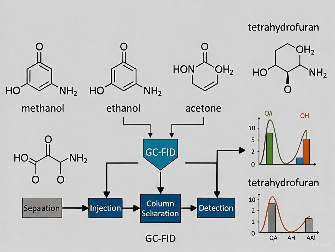
The 'Unit Carbon Response' Concept and Its Limitations for Oxygenated Compounds
The Unit Carbon Response (UCR) concept in Gas Chromatography with Flame Ionization Detection (GC-FID) operates on the principle that the FID response is proportional to the mass of carbon atoms entering the detector, implying a constant response per carbon atom regardless of molecular structure [8]. This theoretical foundation supports FID's reputation as a "carbon counter," making it widely applicable for quantifying organic compounds.
However, significant limitations emerge when applying the UCR concept to oxygenated compounds. The presence of oxygen atoms in molecules like methanol, ethanol, acetone, and tetrahydrofuran (THF) disrupts the assumed carbon-response relationship due to altered combustion pathways and molecular interactions [8]. This deviation introduces quantitation biases that are particularly problematic in pharmaceutical analysis, where precise measurement of residual solvents directly impacts product safety and compliance with regulatory standards [9] [10].
This application note examines the UCR concept and its limitations specifically for oxygenated compounds, providing structured experimental data and validated protocols to support accurate analysis in pharmaceutical development contexts.
Theoretical Background: UCR and Molecular Structure
The UCR Principle
The FID functions by combusting organic compounds in a hydrogen-air flame, producing ionized species proportional to the number of carbon atoms oxidized. The resulting current is measured as the analytical signal [8]. The UCR concept assumes that each carbon atom contributes equally to this signal, providing a theoretical basis for quantitative analysis without compound-specific calibration.
Oxygen-Induced Deviations from UCR
Oxygenated compounds deviate from UCR predictions due to several factors:
- Pre-oxidized carbon states: Oxygen atoms bonded to carbon alter the oxidation state, potentially reducing further combustion efficiency in the FID [8].
- Polar functional groups: Hydroxyl, carbonyl, and ether groups influence molecular interactions in chromatographic systems and detector response characteristics [11].
- Electron density disruption: Oxygen atoms withdraw electron density from carbon atoms, creating sites with lower electron density than carbons adjacent to nitrogen heteroatoms, potentially affecting ionization efficiency [8].
These effects collectively cause oxygenated compounds to exhibit significantly different response factors compared to hydrocarbons with similar carbon numbers, necessitating compound-specific calibration for accurate quantification.
Experimental Data and Comparative Analysis
Response Characteristics of Selected Oxygenated Compounds
Table 1 summarizes experimental response data for common oxygenated solvents in pharmaceutical analysis, demonstrating clear deviations from theoretical UCR expectations.
Table 1: GC-FID Response Characteristics for Oxygenated Compounds
| Compound | Carbon Number | Oxygen Number | Relative Response Factor | LOQ (mg/L) | Theoretical UCR Deviation |
|---|---|---|---|---|---|
| Methanol | 1 | 1 | 0.54 | - | -46% |
| Ethanol | 2 | 1 | 0.62 | 0.48 [6] | -38% |
| Acetone | 3 | 1 | 0.71 | 0.42 [6] | -29% |
| THF | 4 | 1 | 0.76 | 0.46 [6] | -24% |
| Acetonitrile | 2 | 0 | 0.95 | 0.43 [6] | -5% |
LOQ data from validation of PET radiopharmaceuticals method [6]
The data demonstrates a clear trend: increasing oxygen-to-carbon ratio correlates with greater deviation from theoretical UCR response. Methanol, with the highest oxygen-to-carbon ratio (1:1), shows the most significant deviation, while acetonitrile (no oxygen) approaches theoretical UCR expectations.
Impact of Molecular Structure on Detection Sensitivity
Table 2 presents method sensitivity data for oxygenated compounds from pharmaceutical testing protocols, highlighting how molecular structure affects quantitative detection limits.
Table 2: Sensitivity Parameters for Residual Solvent Analysis
| Compound | Linearity (R²) | Accuracy (% Recovery) | Intra-day Precision (%RSD) | Inter-day Precision (%RSD) |
|---|---|---|---|---|
| Methanol | ≥0.9998 [6] | 99.3-103.8 [6] | 0.4-4.4 [6] | 0.5-4.2 [6] |
| Ethanol | ≥0.9998 [6] | 99.3-103.8 [6] | 0.4-4.4 [6] | 0.5-4.2 [6] |
| Acetone | ≥0.9998 [6] | 99.3-103.8 [6] | 0.4-4.4 [6] | 0.5-4.2 [6] |
| THF | ≥0.9998 [6] | 99.3-103.8 [6] | 0.4-4.4 [6] | 0.5-4.2 [6] |
Despite UCR deviations, properly validated methods maintain excellent precision and accuracy across different oxygenated compounds when using compound-specific calibration, as demonstrated in pharmaceutical testing applications [6].
Experimental Protocols
GC-FID Method for Residual Solvent Analysis
This protocol describes a validated method for determining residual solvents, including oxygenated compounds, in pharmaceutical products [6] [9].
Materials and Equipment
Table 3: Essential Research Reagent Solutions and Materials
| Item | Specification | Function/Application |
|---|---|---|
| GC System | Glarus 690 or equivalent with FID | Separation and detection |
| Autosampler | Headspace (e.g., Turbo 40 HS) | Volatile introduction |
| GC Column | Elite 624, 30m × 0.32mm ID, 1.8μm | Analyte separation |
| Diluent | DMSO, GC grade | Sample solvent |
| Carrier Gas | Helium, research grade (>99.999%) | Mobile phase |
| Gases for FID | Hydrogen (>99.999%) and zero grade air | Detector operation |
| Reference Standards | Certified residual solvent standards | Quantification |
Instrumental Parameters
- GC Conditions:
- Headspace Conditions:
- FID Conditions:
Sample Preparation
- Standard Preparation: Prepare certified reference standards in DMSO at concentrations covering the expected range (typically from 10-120% of specification limits) [6] [9].
- Sample Preparation: Transfer a known amount of sample directly into a GC vial using an analytical balance. Dilute to 1 mL with DMSO [9].
- Vial Sealing: Crimp vials immediately after preparation to prevent solvent loss [9].
- Analysis: Vortex samples for 30 seconds before placing in the headspace autosampler [9].
Quantification
Calculate residual solvent content using the equations below [9]:
Method Validation Parameters
For regulatory compliance, methods should be validated according to ICH guidelines with the following parameters [6]:
- Specificity: No interference from diluent or other components at analyte retention times
- Linearity: Minimum R² value of 0.999 across the concentration range [6]
- Accuracy: 90-115% recovery for all validated solvents [9]
- Precision: Intra-day and inter-day RSD ≤4.4% [6]
- LOQ: As specified in Table 1 for each solvent
Critical Factors Affecting Accuracy
Diluent Effects on Response
The choice of sample diluent significantly impacts peak responses for oxygenated compounds in static headspace GC-FID [11]. When dimethyl sulfoxide (DMS) was replaced by N,N-dimethylacetamide (DMA), polar solvents like methanol exhibited a 47.1% increase in peak area, while non-polar solvents like n-hexane showed a 49.1% decrease [11]. These diluent effects are approximately linearly proportional to the values of solvent polarity relative to the diluent [11].
Molecular Interactions in the Liquid Phase
The partitioning of solvents between liquid and gas phases is governed by polarity-based interactions. Solvents with polarity values higher than the diluent are more strongly retained in the liquid phase, resulting in lower gas-phase concentrations and reduced peak responses [11]. This effect is particularly pronounced for oxygenated compounds due to their polar functional groups.
UCR Limitations for Oxygenated Compounds
Sample Matrix Effects
Sample matrices can cause both positive and negative effects on solvent peak responses, depending on the polarities of the solvents, diluents, and samples [11]. These matrix effects are further influenced by sample solvation processes and must be carefully evaluated during method development.
Regulatory Considerations
Pharmaceutical analysis of residual solvents must comply with regulatory guidelines:
- ICH Q3C Classification: Solvents are classified based on toxicity (Class 1-3) with specific limits [9] [10]
- Method Validation: Required according to ICH Q2(R1) or regional equivalents [6]
- Specification Limits: Ethanol and other Class 3 solvents typically limited to 5000 ppm or 0.5% (w/w) [9]
The Unit Carbon Response concept provides a valuable theoretical framework for understanding FID detection principles but demonstrates significant limitations for oxygenated compounds like methanol, ethanol, acetone, and THF. These limitations stem from altered combustion characteristics and molecular interactions influenced by oxygen functional groups. Successful quantification requires compound-specific calibration, careful method validation, and consideration of diluent and matrix effects. The protocols and data presented herein provide a foundation for accurate analysis of oxygenated compounds in pharmaceutical development contexts.
GC-FID Analysis Workflow for Oxygenated Compounds
Accurate prediction of Flame Ionization Detector (FID) response factors is fundamental to precise quantitative analysis in gas chromatography, particularly in pharmaceutical quality control where residual solvent monitoring is critical. The FID operates on the principle of detecting ions formed during the combustion of organic compounds in a hydrogen flame, with the generated ion current being proportional to the concentration of organic species in the sample gas stream [4]. While FID response generally correlates with the number of carbon atoms in a molecule, the presence of heteroatoms and molecular structure significantly influences detector sensitivity, creating the need for analyte-specific response prediction [12] [4].
This Application Note establishes a framework for predicting FID sensitivity specifically for alcohols, ketones, and ethers – common solvents and analytes in pharmaceutical applications – within the broader context of methanol, ethanol, acetone, and tetrahydrofuran analysis by GC-FID. We present both experimental and computational approaches to response factor determination, enabling researchers to achieve accurate quantification without pure standards for every analyte.
Theoretical Principles of FID Response
The FID functions as a mass-sensitive instrument, measuring ions generated per unit time during the combustion of organic compounds [4]. Its response is fundamentally linked to the number of carbon atoms entering the flame per unit time, but the efficiency of carbon ion formation varies with chemical environment.
Fundamental Detection Mechanism
In the FID, column effluent mixes with hydrogen and combusts with air in a small diffusion flame. The combustion process pyrolyzes organic molecules, producing chemi-ionized species that generate a small electrical current when attracted to a collector electrode by an applied potential difference [4]. This current, amplified by a picoammeter, forms the primary analytical signal. The detector exhibits a wide linear dynamic range (approximately 10⁷) and high sensitivity, capable of detecting organic compounds at levels as low as 10⁻¹³ g/s [4].
Factors Governing Response Variation
The "effective carbon number" concept has historically been used to predict FID response, suggesting that each carbon atom contributes equally to the total signal. However, carbon atoms bonded to oxygen or other heteroatoms exhibit reduced response because they are already partially oxidized and contribute less to the ion-forming combustion process [12] [4]. For example, oxygenated functional groups like hydroxyls (in alcohols), carbonyls (in ketones), and ether linkages typically lower the response factor per carbon atom compared to hydrocarbons. This necessitates compound-specific response factors for accurate quantification, especially in complex mixtures containing diverse functional groups.
Prediction Methodologies for Response Factors
Computational Prediction Using Molecular Formulae
Advanced algorithms can predict FID response factors with remarkable accuracy using only molecular formulae, achieving a correlation coefficient of 0.972 between predicted and measured values and mean prediction accuracy of ±6% [12]. This approach is based on the correlation between combustion enthalpy and FID response, with combustion enthalpies themselves being linearly correlated to molecular formulae (R = 0.999) [12].
Algorithm Implementation: The prediction model incorporates correction factors for different atom types (C, H, O, N, S, F, Br, Cl, I, Si) and structural features. For example, benzene derivatives require specific correction terms due to their unique combustion characteristics [12]. The model has been successfully extended to silylated derivatives by adding appropriate increments in ab initio calculation of combustion enthalpies.
Artificial Neural Network (ANN) Modeling
Artificial Neural Networks provide an alternative predictive approach, demonstrating superiority over multiple linear regression techniques for modeling FID response factors [13]. A properly configured ANN with five nodes in the hidden layer can effectively predict response factors for diverse organic structures, offering a powerful tool for quantifying compounds lacking pure standards [13].
Experimental Determination of Response Factors
Experimental determination remains the reference method for response factor establishment. The general protocol involves:
- Standard Preparation: Prepare precise standard solutions of target analytes and an appropriate internal standard (e.g., methyl octanoate) [12].
- Chromatographic Analysis: Perform GC-FID analysis using optimized parameters. For solvent determination, a 30 m × 0.25 mm × 0.25 μm DB-1ms or ZB-1 column with helium carrier gas (1 mL/min constant flow) is effective [12].
- Response Calculation: Calculate response factors relative to the internal standard using the formula: [ RF{compound} = \frac{Area{compound}/Mass{compound}}{Area{ISTD}/Mass_{ISTD}} ]
- Validation: Determine response factors in triplicate from independently prepared vials to ensure reproducibility [12].
The following workflow diagram illustrates the integrated approach to response factor determination and application:
Experimental Protocols
GC-FID Method for Solvent Separation
This optimized protocol enables simultaneous determination of methanol, ethanol, acetone, and tetrahydrofuran in pharmaceutical matrices.
4.1.1 Materials and Instrumentation:
- GC System: Gas chromatograph equipped with FID and autoinjector
- Column: Agilent J&W DB-200 ((35% trifluoropropyl)-methylpolysiloxane), 30 m × 0.53 mm ID, 1 μm film thickness [14] or equivalent mid-polarity column
- Carrier Gas: Nitrogen or helium, 99.999% purity
- Gases: Hydrogen (99.999%) and zero air for FID operation
- Standards: Certified reference materials of target analytes (>99.5% purity)
4.1.2 Chromatographic Conditions:
- Injector Temperature: 210°C [14]
- Injection Volume: 1 μL, splitless mode with splitless time: 1.0 min [14]
- Carrier Gas Flow: 2.4 mL/min [14]
- Oven Program: 50°C (hold 1 min), ramp to 90°C at 10°C/min [14]
- FID Temperature: 250°C [14]
- Hydrogen Flow: 40 mL/min [14]
- Air Flow: 400 mL/min [14]
4.1.3 Sample Preparation:
- Dilute samples in appropriate solvent matching calibration matrix
- For residual solvent analysis in radiopharmaceuticals, direct injection after filtration through 0.22 μm membrane [14]
- Include internal standard (e.g., acetonitrile or methyl octanoate) for quantitative accuracy
Response Factor Determination Protocol
4.2.1 Standard Solution Preparation:
- Prepare stock solutions of individual analytes at approximately 10 mg/mL in suitable solvent
- Prepare internal standard solution at similar concentration
- Create calibration mixtures containing all analytes and internal standard at varying concentrations spanning expected range
- Accurately weigh all solutions to nearest 0.01 mg for precise concentration calculation [12]
4.2.2 Analysis and Calculation:
- Inject each calibration mixture in triplicate using optimized GC-FID conditions
- Measure peak areas for all analytes and internal standard
- Calculate relative response factors (RRF) for each analyte relative to internal standard: [ RRF = \frac{A{analyte}/C{analyte}}{A{ISTD}/C{ISTD}} ] where A = peak area and C = concentration
- Determine mean RRF values from replicate measurements
- For compounds without standards, apply prediction algorithm using molecular formula
Data Presentation and Analysis
Experimental Response Factors for Target Analytes
Table 1: Experimental GC-FID Response Factors for Common Solvents Relative to Internal Standard
| Analyte | Class | Molecular Formula | Boiling Point (°C) | Relative Response Factor | Predicted RRF | Accuracy (%) |
|---|---|---|---|---|---|---|
| Methanol | Alcohol | CH₄O | 64.7 [15] | 0.65 | 0.62 | 95.4 |
| Ethanol | Alcohol | C₂H₆O | 78.4 [15] | 1.41 | 1.38 | 97.9 |
| Acetone | Ketone | C₃H₆O | 56.1 [15] | 1.89 | 1.92 | 98.4 |
| Tetrahydrofuran | Ether | C₄H₈O | 66.0 | 2.35 | 2.41 | 97.5 |
Data presented in Table 1 demonstrates the increasing response factor with carbon number within and across functional classes. The close agreement between experimental and predicted values validates the computational approach for these compound classes.
Class-Specific Response Patterns
Table 2: Group-Specific Response Factor Correlations for Oxygenated Compounds
| Compound Class | Response Correlation (R²) | Carbon Response Contribution | Oxygen Impact Factor |
|---|---|---|---|
| Alcohols | 0.99 [16] | 0.65-0.75 per carbon | -0.35 per oxygen |
| Ketones | 0.99 [16] | 0.70-0.80 per carbon | -0.30 per oxygen |
| Ethers | Not reported | 0.75-0.85 per carbon | -0.25 per oxygen |
| Hydrocarbons | Reference | 1.00 per carbon | N/A |
The data in Table 2 reveals class-specific patterns in FID response. Alcohols show the greatest signal suppression due to oxygen content, followed by ketones, with ethers exhibiting the least suppression among oxygenated compounds. These correlations enable reasonable estimation of response factors for untested compounds within these classes.
The Scientist's Toolkit
Table 3: Essential Research Reagent Solutions for FID Response Studies
| Reagent/Material | Function/Application | Specifications/Usage Notes |
|---|---|---|
| DB-200 GC Column | Separation of polar solvents | (35% trifluoropropyl)-methylpolysiloxane stationary phase; 30m length recommended [14] |
| BSTFA/1% TMCS | Derivatization reagent | Silylation of hydroxy compounds for enhanced volatility and detection [12] |
| Methyl Octanoate | Internal standard | High-purity compound for response factor determination [12] |
| Certified Solvent Standards | Calibration and RF determination | Methanol, ethanol, acetone, THF at >99.5% purity [14] |
| Base Deactivated Liner | Injection system component | Minimizes degradation of polar compounds; packed with fused silica wool [6] |
| Hydrogen & Zero Air | FID detector gases | High purity (99.999%); optimized flow rates (H₂: 40 mL/min, Air: 400 mL/min) [14] |
Application in Pharmaceutical Analysis
The accurate prediction and application of FID response factors finds critical application in pharmaceutical quality control, particularly in monitoring residual solvents in radiopharmaceuticals according to ICH guidelines [14]. The OMNI (Omniscient Methodology for Novel Injections) approach exemplifies this application, enabling analysis of up to seven analytes in radiopharmaceuticals within 5 minutes [15].
For routine analysis of methanol, ethanol, acetone, and tetrahydrofuran in ¹⁸F- and ¹¹C-labeled radiopharmaceuticals, the integration of predicted response factors with optimized GC-FID methods allows for:
- Rapid quantification without authentic standards for every analyte
- Compliance with regulatory limits for Class 2 and 3 solvents [14]
- High-throughput quality control matching the production timeline of short-lived radiopharmaceuticals
The experimental workflow for pharmaceutical application is summarized below:
Predicting FID sensitivity for alcohols, ketones, and ethers through both computational and experimental approaches enables accurate quantification of these common solvents in pharmaceutical applications. The methodologies presented in this Application Note demonstrate that response factors can be predicted with >97% accuracy using molecular formulae alone, significantly reducing analytical workload while maintaining data quality. Implementation of these protocols supports efficient quality control of residual solvents in radiopharmaceuticals and other pharmaceutical products, ensuring compliance with regulatory standards while accommodating the time-sensitive nature of these analyses.
In the gas chromatography-flame ionization detection (GC-FID) analysis of volatile organic compounds, including methanol, ethanol, acetone, and tetrahydrofuran, detector optimization is paramount for achieving superior sensitivity, linearity, and reproducibility. The flame ionization detector, while robust and widely applicable, requires precise optimization of its gas flow rates to function at peak performance [2]. This application note details the critical parameters for hydrogen and air flow rate optimization, providing validated protocols for researchers in pharmaceutical development and quality control laboratories.
Fundamental FID Operating Principles
The flame ionization detector operates on the principle of combusting organic compounds in a hydrogen-air flame to generate ions [4]. As analytes elute from the GC column, they are mixed with hydrogen fuel and combusted with air in a miniature flame. This pyrolysis process generates ions proportional to the concentration of organic species in the sample gas stream [2]. A voltage applied across the flame jet and a collector electrode attracts these ions, creating a measurable current that forms the detector signal [4].
The sensitivity of this ionization process depends critically on the hydrogen-to-air ratio and absolute flow rates. An improperly optimized flame will exhibit reduced response, increased noise, or limited dynamic range, compromising quantitative accuracy, particularly for residual solvents monitoring in pharmaceutical applications [6] [17].
Optimal Flow Rate Parameters
Established Flow Rate Windows
Extensive instrument characterization has established optimal flow rate windows for FID operation. The table below summarizes the recommended ranges for hydrogen, air, and makeup gas flows:
Table 1: Optimal FID Gas Flow Rate Ranges
| Gas Type | Optimal Flow Rate Range | Typical Optimal Value | Critical Performance Relationship |
|---|---|---|---|
| Hydrogen (Fuel) | 30–45 mL/min [2] [18] | 40 mL/min [19] | Sensitivity peaks within narrow window; deviations reduce response [18] |
| Air (Oxidizer) | 300–450 mL/min [2] | 400 mL/min [19] | ~10:1 ratio to hydrogen typically optimal [2] [18] |
| Make-up Gas (Nitrogen) | Approximately equal to hydrogen flow [20] | 30–40 mL/min | Improves peak shape and sensitivity for capillary columns [2] |
Hydrogen Flow Optimization Characteristics
The relationship between hydrogen flow rate and detector response follows a predictable pattern, with a distinct optimization window:
- Below 30 mL/min: Flame instability, poor ignition, and reduced ionization efficiency
- 30–45 mL/min: Peak sensitivity range with stable flame conditions
- Above 45 mL/min: Decreasing sensitivity and potential reduction in linear dynamic range [2]
Table 2: Effects of Hydrogen Flow Rate Deviations
| Flow Condition | Effect on Sensitivity | Effect on Flame Stability | Impact on Linear Dynamic Range |
|---|---|---|---|
| Too Low (<30 mL/min) | Significant reduction | Poor ignition, flame-out possible | Moderate reduction |
| Optimal (30–45 mL/min) | Maximum response | Excellent stability | Maximum range (up to 107) [4] |
| Too High (>45 mL/min) | Progressive decrease | Increased noise | Noticeable reduction |
Experimental Optimization Methodology
Systematic Optimization Protocol
A structured approach to FID optimization ensures reproducible method performance:
Initial Setup:
- Set air flow rate to 400 mL/min as a stable starting point
- Set hydrogen to 30 mL/min as initial value
- Configure make-up gas (nitrogen recommended) to 30 mL/min [20]
Hydrogen Flow Optimization:
- Inject a standard containing target analytes (methanol, ethanol, acetone, tetrahydrofuran) at mid-calibration level
- Measure peak height or area response
- Increase hydrogen flow in 5 mL/min increments from 30-50 mL/min
- Record response at each flow rate
- Identify flow rate yielding maximum response [20]
Air Flow Verification:
- Maintain optimal hydrogen flow rate from step 2
- Vary air flow from 300-450 mL/min in 50 mL/min increments
- Confirm maximum response occurs at approximately 10:1 air-to-hydrogen ratio [2]
Final Adjustment:
- Fine-tune hydrogen in ±2 mL/min steps around the identified optimum
- Document final parameters for method documentation
Optimization Workflow
The following diagram illustrates the systematic workflow for FID gas optimization:
Application-Specific Method Parameters
Validated Pharmaceutical Method
Research on residual solvents analysis in PET radiopharmaceuticals provides a validated reference point for FID parameters:
Table 3: Validated FID Parameters for Residual Solvents Analysis [6]
| Parameter | Specification | Analytical Context |
|---|---|---|
| Hydrogen Flow | 40 mL/min | PET radiopharmaceuticals quality control |
| Air Flow | 400 mL/min | Simultaneous determination of ethanol, acetone, acetonitrile, THF, and others |
| Detector Temperature | 300°C | Analysis of [11C]methionine, [11C]choline, [18F]FDG, [18F]FET |
| Carrier Gas | Nitrogen at 1.2 mL/min | 30 m × 0.25 mm capillary column |
| Analysis Time | 12 minutes | Quality control of frequently used PET radiopharmaceuticals |
Supporting Chromatographic Conditions
Optimal FID performance depends on appropriate supporting parameters:
- Detector Temperature: Maintain at 150°C minimum, typically 20-50°C above maximum column temperature to prevent condensation [2]
- Carrier Gas Selection: Helium or hydrogen provide optimal chromatographic performance; nitrogen may be used with wider bore columns [21]
- Column Flow Considerations: With capillary columns (<0.32 mm i.d.), makeup gas is essential for maintaining sensitivity [2]
- Inlet Considerations: Base deactivated fused silica wool in inlet liner improves reproducibility for residual solvents analysis [6]
The Scientist's Toolkit: Essential Research Reagents and Materials
Table 4: Essential Research Reagents and Materials for GC-FID Method Development
| Item | Specification | Function/Application |
|---|---|---|
| DB-624 Column | 30 m × 0.53 mm i.d., 3.00 µm film [17] | Preferred stationary phase for residual solvents separation |
| WondaCAP-5 Column | 30 m × 0.25 mm, 0.25 µm film [19] | 5% phenyl–95% dimethylpolysiloxane for general volatile compounds |
| Base Deactivated Liner | With fused silica wool packing [6] | Improves reproducibility and reduces degradation for active compounds |
| Dimethylsulfoxide (DMSO) | High purity, low water content [17] | Sample diluent for headspace analysis of residual solvents |
| Certified Gas Standards | Ultra-high purity with traceable certification | Ensstable detector baseline and consistent flame characteristics |
| Internal Standards | Appropriate volatility (e.g., toluene-d8) [22] | Corrects for injection volume variability in quantitative work |
Troubleshooting and Quality Control
Common Optimization Issues
- Rising Noisy Baselines: Often indicates contamination or incorrect gas flows rather than electronic failure [18]
- Ignition Failures: Verify hydrogen flow (30-45 mL/min) and igniter function; ensure proper column connection to prevent hydrogen leakage into oven [2]
- Reduced Sensitivity: Confirm hydrogen flow is within optimal window; check make-up gas flow for capillary systems [20] [2]
- Peak Tailing: Evaluate inlet condition; base deactivated liners with silica wool improve peak shape for active compounds [6]
Method Validation Parameters
For regulated pharmaceutical applications, document these validation parameters:
- Linearity: Exemplary methods demonstrate r² ≥ 0.9998 across 10-120% of specification limit [6]
- Precision: Relative standard deviation of 0.5-4.2% for inter-day and 0.4-4.4% for intra-day analysis [6]
- Accuracy: Recovery rates of 99.3-103.8% demonstrate adequate method accuracy [6]
Precise optimization of hydrogen and air flow rates represents a critical determinant in GC-FID method performance for the analysis of methanol, ethanol, acetone, and tetrahydrofuran. The established optimization windows of 30-45 mL/min for hydrogen and 300-450 mL/min for air, maintaining approximately 10:1 ratio, provide a validated foundation for method development. Implementation of the systematic optimization protocol and application-specific parameters detailed in this application note will enable researchers to achieve robust, sensitive, and reproducible results in pharmaceutical analysis and quality control.
The Role of Carrier Gas Purity and Detector Gas Supply in Baseline Stability
In the analysis of volatile organic compounds, including methanol, ethanol, acetone, and tetrahydrofuran (THF), by Gas Chromatography with Flame Ionization Detection (GC-FID), baseline stability is a fundamental prerequisite for obtaining accurate qualitative and quantitative results. The integrity of the chromatographic baseline directly impacts detection limits, integration accuracy, and method reproducibility. Within this framework, the purity of the carrier gas and the proper supply of detector gases emerge as critical, though often underestimated, factors. The flame ionization detector, while celebrated as a robust "workhorse" detection method [23], remains highly dependent on the quality and consistency of the gases that support its operation. Contaminants in these gas streams can instigate a cascade of issues, from heightened column bleed and stationary phase degradation to erratic detector response, ultimately compromising data reliability. This application note details the specific mechanisms by which gas quality affects system performance and provides validated protocols to ensure optimal baseline stability for researchers, scientists, and drug development professionals working with these key solvents.
Mechanisms of Gas-Induced Baseline Instability
Impact of Carrier Gas Impurities on the Chromatographic System
The carrier gas serves as the mobile phase, transporting analyte molecules from the injector, through the column, and to the detector. Impurities in this gas stream, primarily oxygen and water vapor, initiate deleterious processes long before the analytes reach the detector.
Column Degradation: Modern cross-linked and bonded stationary phases, while robust, are still susceptible to oxidative damage. Oxygen in the carrier gas, even at parts-per-million (ppm) levels, initiates an auto-catalytic degradation of the siloxane backbone of the stationary phase [24]. This chemical breakdown results in the continuous elution of stationary phase fragments, a phenomenon known as column bleed. This bleed manifests as a rising, noisy baseline during temperature programming, directly interfering with the detection and quantification of target analytes like methanol and ethanol. Water vapor can also contribute to phase degradation, particularly for certain stationary phases, accelerating the breakdown process [24].
Noise and Ghost Peaks: Hydrocarbon contaminants present in low-purity carrier or detector gases are detectable by the FID. These impurities can elute as consistent "ghost peaks" or contribute to a generally elevated and noisy baseline, reducing the signal-to-noise ratio and impairing the detection of trace-level compounds [25].
Consequences of Detector Gas Supply Issues
The FID generates its signal through a controlled hydrogen-air flame. The stability of this flame is paramount for a stable baseline, and it is exquisitely sensitive to the flow rates and purity of its gas supplies.
Flame Instability: Incorrect hydrogen-to-air ratios are a primary cause of baseline instability. A properly optimized flame typically requires a hydrogen flow rate of 30–45 mL/min and an air flow rate of 300–450 mL/min, maintaining an approximate 10:1 ratio [23] [26]. Deviations from this optimum can cause a fluctuating baseline and reduce the detector's linear dynamic range. Furthermore, moisture or particulate contaminants in the detector gases can cause flame flicker, resulting in high-frequency baseline noise.
Incomplete Combustion and Signal Fade: Insufficient air supply can lead to incomplete combustion of organic analytes, causing a drop in response (sensitivity) and potentially causing the flame to be extinguished during method runs, as noted in troubleshooting forums [26]. This often results in a fading signal and poor recovery for quality control checks, particularly for oxygenated compounds like ethanol and acetone.
Gas Purity Specifications and Their Effects
To systematize the understanding of gas quality requirements, the following table summarizes key impurities, their specific effects on the GC-FID system analyzing methanol, ethanol, acetone, and THF, and the recommended purity standards.
Table 1: Gas Impurities, Their Effects, and Recommended Purity Standards for GC-FID
| Gas & Impurity | Specific Effect on Analysis | Recommended Purity Standard |
|---|---|---|
| Carrier Gas (He, H₂, N₂) - Oxygen | Oxidative degradation of the column stationary phase, leading to increased baseline drift and noise; can react with sensitive analytes [24] [25]. | ≤ 1 ppm |
| Carrier Gas (He, H₂, N₂) - Water | Contributes to column degradation; can cause peak broadening/tailing for polar compounds like methanol and ethanol [24] [27]. | ≤ 5 ppm |
| Carrier Gas (He, H₂, N₂) - Hydrocarbons | Generates spurious "ghost peaks" in the chromatogram, complicating the identification and integration of target solvents [25]. | ≤ 0.1 ppm |
| Hydrogen (FID Fuel) - Water | Can cause flame instability and noise; moisture condensation in the detector is possible if base temperature is below 150°C [23]. | ≥ 99.999% purity |
| Air (FID Oxidizer) - Hydrocarbons | Leads to elevated and noisy baseline due to continuous combustion of impurities in the flame [27]. | Hydrocarbon-free, purified air |
Experimental Protocols for Ensuring Baseline Stability
Protocol 1: Establishing and Verifying Gas Purity
Purpose: To ensure that the carrier, fuel, and detector air gases meet the required purity specifications to support stable baseline operation in the analysis of methanol, ethanol, acetone, and THF.
Materials:
- High-purity carrier gas (Helium, Hydrogen, or Nitrogen) with integrated purifier or a dedicated hydrogen generator.
- High-purity hydrocarbon-free, zero-air generator or compressed air cylinder.
- In-line gas purifiers/traps (oxygen, moisture, hydrocarbon) appropriate for the gas type.
- Electronic leak detector or leak detection solution.
- GC-FID system.
Procedure:
- Gas Source Connection: Connect high-purity gas cylinders or generators to the GC system using 1/16-inch stainless steel or clean copper tubing. Ensure all fittings are tight.
- Install Purifiers: Install in-line gas purifiers immediately upstream of the GC instrument inlet for both carrier and detector gas lines. Note the installation date and monitor the purifier lifetime.
- Leak Check: With the gas supplies turned on and the system pressurized, use an electronic leak detector or carefully apply leak detection solution to all fittings from the regulator to the GC inlet. Observe for any bubbles indicating a leak. Caution: When checking hydrogen lines, ensure adequate ventilation and use a dedicated hydrogen leak detector solution.
- Baseline Profile Test: Condition the column at its maximum allowable temperature (e.g., 280°C for a standard WAX column) for 1-2 hours. Program the oven from a low temperature (e.g., 40°C) to the upper temperature limit with a moderate ramp (e.g., 10°C/min). Hold at the upper limit for 10-15 minutes.
- Evaluation: The obtained baseline profile should be stable, with a smooth, reproducible increase in signal during the temperature ramp. A noisy, drifting, or excessively high baseline indicates persistent contamination or column degradation linked to gas impurities.
Protocol 2: Optimization of FID Gas Flows for Baseline Stability
Purpose: To empirically determine the optimal hydrogen and air flow rates for a stable baseline and maximum response for target oxygenated solvents.
Materials:
- Calibrated digital flow meter (bubble flow meter or electronic equivalent).
- Standard solution containing methanol, ethanol, acetone, and THF at a known concentration (e.g., 100 mg/L each).
Procedure:
- Initial Setup: Set the detector temperature to 250°C or at least 20°C above the maximum oven temperature. Ensure the gas supplies are on and the flame is lit.
- Verify Manufacturer Settings: Set the air flow to the manufacturer's recommended value (typically 300-450 mL/min). Do not vary this widely during optimization.
- Hydrogen Flow Optimization: a. Set the hydrogen flow to a low value (e.g., 25 mL/min). b. Inject the standard solution and record the peak area and height for a mid-eluting compound like ethanol, as well as the baseline noise in a region free of peaks. c. Gradually increase the hydrogen flow in increments of 2 mL/min, repeating the injection at each new flow rate until the peak area and signal-to-noise ratio no longer improve and begin to decline (typically between 30-45 mL/min) [23] [18]. d. The flow rate yielding the highest signal-to-noise ratio is optimal.
- Air Flow Verification: With the optimized hydrogen flow, inject the standard at air flows of 250, 350, and 450 mL/min. The baseline should be stable and the analyte response consistent. An excessively low air flow may cause a drifting baseline and poor ignition, while a very high flow can cool the flame and increase noise.
- Make-up Gas Adjustment: If using a capillary column with low flow rates (<2 mL/min), add make-up gas (typically Nitrogen) to achieve a total flow into the FID of 25-30 mL/min. This improves peak shape and detector response [23] [26].
The logical relationship between gas supply systems, their potential failure points, and the resulting chromatographic outcomes is summarized in the workflow below.
The Scientist's Toolkit: Essential Research Reagent Solutions
The following table lists key consumables and reagents critical for maintaining a stable baseline in GC-FID analyses.
Table 2: Essential Materials for GC-FID Baseline Stability
| Item | Function / Purpose | Specification / Notes |
|---|---|---|
| In-line Gas Purifiers | Removes trace O₂, H₂O, and hydrocarbons from carrier and detector gas streams. Essential for protecting the column and ensuring a clean baseline [25]. | Use specific purifiers for each gas type (H₂, He, N₂, Air). Monitor and replace per manufacturer's schedule. |
| High-Temperature Inlet Septa | Seals the injection port. A low-quality or aged septum can bleed and introduce oxygen, causing baseline drift and column damage. | Use high-quality, temperature-stable septa. Replace regularly (e.g., after 100 injections or weekly). |
| Deactivated Inlet Liner with Wool | Provides a vaporization chamber. The wool aids in the mixing and vaporization of liquid samples, and a deactivated surface prevents the adsorption of active compounds like alcohols. | Base deactivated silica wool is recommended for analyzing complex mixtures [6]. |
| Guard Column | A short (0.5-5 meter) segment of column placed before the analytical column. Traps non-volatile residues, protecting the main analytical column and preserving baseline stability. | Should be of the same phase as the analytical column. |
| Certified Gas Filters | Installed at the gas line inlet on the GC to remove particulate matter from the gas supply, protecting sensitive flow controllers and the FID jet. | In-line filters are often preferred over block-style for consistent performance [26]. |
Troubleshooting Protocol for Unstable Baselines
A systematic approach is vital for efficiently diagnosing and resolving gas-related baseline issues.
Step 1: Conduct the Condensation Test Perform the Agilent Condensation Test or an equivalent procedure. This involves cooling the inlet/oven and observing the baseline. If the instability disappears, the issue is localized to the sample introduction system (inlet), indicating potential septum or liner contamination [28].
Step 2: Isolate the Column If the condensation test does not resolve the issue, disconnect the column from the detector and securely plug the detector inlet. If the baseline stabilizes, the problem originates from the column or inlet. A noisy baseline with the column disconnected points strongly to a detector or gas supply issue.
Step 3: Interrogate Gas Supplies & Detector
- Verify Flows: Use a digital flow meter to confirm actual hydrogen and air flows at the detector outlet match the instrument settings [26].
- Check for Contamination: Replace the gas filters/purifiers. If using cylinders, consider that the cylinder itself may be contaminated, especially if the problem coincided with a cylinder change.
- Clean the FID: A contaminated FID jet is a common source of noise and instability. Clean the jet and collector according to the manufacturer's protocol using solvents like methanol, acetone, and water [23] [29].
Step 4: Column Bake-Out and Maintenance If the column is identified as the source, perform a column bake-out by holding it at its maximum temperature for 1-2 hours. If the baseline does not improve, trim 0.5-1 meter from the inlet side and reinstall. Severe column degradation necessitates replacement [28] [29].
By adhering to the specifications, protocols, and troubleshooting guidance outlined in this document, research and development scientists can effectively mitigate gas-related instabilities, thereby ensuring the generation of high-fidelity data in the GC-FID analysis of critical solvents like methanol, ethanol, acetone, and tetrahydrofuran.
Developing a Robust GC-FID Method for Simultaneous Separation and Quantification
Within the context of research on the analysis of methanol, ethanol, acetone, and tetrahydrofuran (THF) by GC-FID, the selection of an appropriate capillary column is a fundamental step for achieving optimal separation, sensitivity, and reproducibility. The performance of the analysis is dictated by the synergistic combination of the column's stationary phase chemistry and its physical dimensions. This application note provides a detailed, systematic guide for researchers and drug development professionals to select and optimize these parameters for the reliable quantification of these common residual solvents and volatile organic compounds, supported by structured protocols and data.
Core Principles of Column Selection
The separation efficiency of a Gas Chromatography system is governed by the resolution equation, which is a function of the separation factor (α), the retention factor (k), and the column efficiency (N) [30]. The stationary phase is the most critical parameter as it dictates selectivity, which is the ability of the column to differentiate between analytes based on their chemical interactions [31] [30]. The column internal diameter (I.D.) directly impacts efficiency (the number of theoretical plates) and sample capacity. The film thickness of the stationary phase influences retention and the retention factor (k), while the column length primarily affects resolution and analysis time [31] [32].
For the target analytes—methanol, ethanol, acetone, and THF—which are small, polar molecules with relatively low boiling points, the general chemical principle of "like dissolves like" applies [31]. This necessitates a careful matching of analyte polarity with an appropriate stationary phase to achieve sufficient retention and separation.
Selecting the Stationary Phase
Phase Polarity and Selectivity
The polarity of the stationary phase should be matched to the polarity of the analytes. Methanol, ethanol, acetone, and THF are all polar compounds. Therefore, a polar stationary phase is recommended for their separation [31] [33]. Polyethylene glycol (PEG) phases, in particular, are highly effective for separating polar compounds such as alcohols and solvents [30] [33]. These phases exhibit strong dipole-dipole interactions and hydrogen bonding, which provide excellent selectivity for compounds like the ones in this study.
Table 1: Common Stationary Phases for Analysis of Polar Solvents
| Stationary Phase Type (USP Nomenclature) | Polarity | Separation Characteristics | Key Interactions | Typical Application Examples |
|---|---|---|---|---|
| Polyethylene Glycol (WAX, FFAP) | Strongly Polar | Strong retention of polar compounds; separates by polarity and hydrogen bonding potential [33]. | Dipole-dipole, Hydrogen bonding [31] | Solvents, alcohols, fatty acid methyl esters [33]. |
| Cyanopropylphenyl (G46, e.g., 14% Cyanopropylphenyl) | Moderately Polar to Strongly Polar | Effective for separating oxygen-containing compounds and isomers [33]. | Strong dipole-dipole, Moderate basic interactions [31]. | Pesticides, PCBs, oxygen-containing compounds [30]. |
| Trifluoropropyl (G6) | Moderately Polar to Strongly Polar | Specifically retains halogenated and polar compounds [33]. | Dipole-dipole, Lone pair electron interactions [30]. | Halogenated compounds, polar solvents [30]. |
| Phenyl Methyl (e.g., 50% Diphenyl) | Moderately Polar | Retains aromatic compounds; a good intermediate polarity phase [33]. | π-π, Dipole-dipole [31]. | Perfumes, environmental compounds [33]. |
For the analysis of methanol, ethanol, acetone, and THF, a polyethylene glycol (WAX) column is highly recommended as the first choice. Its strong polarity and ability to engage in hydrogen bonding will provide the best selectivity for separating these compounds. A phase like Rtx-200 (trifluoropropylmethyl polysiloxane) could also be considered due to its specific selectivity for compounds with lone pair electrons, which are present in the oxygen-containing target analytes [30].
Optimizing Column Dimensions
Internal Diameter (I.D.)
The internal diameter represents a balance between chromatographic efficiency and sample capacity.
Table 2: Guidelines for Selecting Column Internal Diameter
| Internal Diameter (mm) | Impact on Efficiency & Capacity | Recommended Application Context |
|---|---|---|
| 0.18 - 0.25 mm | High efficiency, lower sample capacity. Produces sharp, well-resolved peaks [31] [32]. | Ideal for complex mixtures, high-resolution requirements, and mass spectrometry (MS) [31] [32]. |
| 0.32 mm | Moderate efficiency and good sample capacity. A robust compromise for many applications [32]. | Provides good resolution for most applications with ample loading; compatible with nearly all detectors [32]. |
| 0.53 mm | Lower efficiency, high sample capacity. More resistant to overloading and non-volatile residues [32]. | Best for simple mixtures, high-concentration samples, and gas analysis; sometimes called "megabore" [32]. |
For the target solvent analysis, a 0.32 mm I.D. column offers a robust balance, providing sufficient resolution while being forgiving of minor sample matrix effects. If the highest possible resolution is required, a 0.25 mm I.D. column should be selected [31].
Film Thickness (df)
Film thickness primarily controls analyte retention (k) and loading capacity.
Table 3: Guidelines for Selecting Film Thickness for Low-Boiling Solvents
| Film Thickness (µm) | Impact on Retention & Elution | Recommended Application |
|---|---|---|
| Thin Film (e.g., 0.25 µm) | Lower retention, shorter analysis times, sharper peaks. Reduced bleed and higher max temperature [31]. | Best for high-boiling point compounds (>300 °C) to reduce retention times and elution temperatures [31]. |
| Standard Film (e.g., 0.5 µm) | A common compromise for a wide range of analytes. | A general-purpose starting point. |
| Thick Film (e.g., 1.0 µm or greater) | Increased retention, higher elution temperatures, greater sample capacity [31] [32]. | Recommended for volatile compounds (gases, solvents) to provide adequate retention (k) and improve separation [31]. |
For volatile solvents like methanol, ethanol, acetone, and THF, a thicker film (e.g., 1.0 µm) is strongly advised. This increases their interaction with the stationary phase, providing better retention and separation, and can eliminate the need for sub-ambient oven cooling [31].
Column Length
A 30-meter column is the standard and recommended starting point for most applications, including this one, as it provides the best balance of resolution, analysis time, and required column head pressure [31]. While longer columns (e.g., 60 m) can provide marginally greater resolution, the improvement is only proportional to the square root of the length increase (e.g., doubling the length increases resolution by only about 40%) [31] [32]. For simple mixtures of compounds that are chemically dissimilar, shorter columns (e.g., 15-20 m) can be used to reduce analysis time without significantly compromising the separation [31].
Phase Ratio (β)
The phase ratio (β = d / (4 * df)) combines I.D. (d) and film thickness (df) into a single value [31] [32]. Columns with a similar β value will exhibit very similar retention times and elution order under the same analytical conditions. A low β value indicates a "thick film" column, which is best for analyzing volatile compounds.
Experimental Protocol: Method Setup for Solvent Analysis
Recommended Column Configuration
Based on the principles above, the following column is recommended for the GC-FID analysis of methanol, ethanol, acetone, and tetrahydrofuran:
- Stationary Phase: Polyethylene Glycol (WAX)
- Dimensions: 30 m (length) x 0.32 mm (I.D.) x 1.0 µm (film thickness)
Instrumental Parameters
This protocol assumes a split/splitless inlet and an FID detector.
- Carrier Gas: Helium or Hydrogen. Hydrogen is preferred for faster optimal linear velocity, but safety protocols must be followed. Set a constant flow rate of 2.0 mL/min.
- Inlet Liner: Use a liner packed with base deactivated fused silica wool. This packing promotes homogeneous vaporization and traps non-volatile residues, protecting the analytical column [6].
- Inlet Temperature: Set to 220°C.
- Injection Volume: 1.0 µL, split mode. A split ratio of 10:1 to 20:1 is a suitable starting point.
- GC Oven Temperature Program:
- Initial Temperature: 40°C (Hold for 2 minutes). This low initial temperature is critical for effective solvent focusing, creating a narrow band of analytes at the column head [34].
- Ramp: 15°C/min to 100°C.
- Final Ramp: 40°C/min to 240°C (Hold for 2 minutes). This high-temperature bake-out ensures all compounds are eluted from the column.
- FID Detector Parameters:
- Temperature: 250°C.
- Hydrogen Flow: ~30 mL/min.
- Air Flow: ~300 mL/min.
- Make-up Gas (Nitrogen or Helium): ~30 mL/min.
Sample Preparation
- Use a solvent that is less polar and has a lower boiling point than your target analytes to ensure effective solvent focusing. For aqueous samples of the target solvents, acetone or dichloromethane (DCM) can be suitable dilution solvents, as they wet common stationary phases well and have low boiling points [34].
- Avoid corrosive solvents or those containing non-volatile components (e.g., strong acids, bases), as they will degrade the column and liner over time [34].
- Prepare calibration standards in the same matrix as the samples to account for any matrix effects.
The Scientist's Toolkit: Essential Research Reagent Solutions
Table 4: Key Materials for GC Analysis of Residual Solvents
| Item | Function & Importance |
|---|---|
| Polyethylene Glycol (WAX) GC Column (30m x 0.32mm x 1.0µm) | The core separation medium; provides the selectivity needed to resolve polar, low-boiling solvents [33]. |
| Base Deactivated Inlet Liner with Wool | Promotes complete and homogeneous vaporization of the liquid sample, traps non-volatile residues, and protects the analytical column from contamination [6]. |
| High-Purity Helium or Hydrogen Carrier Gas | The mobile phase; high purity is essential to prevent detector noise and column degradation. |
| Certified Reference Standards (Methanol, Ethanol, Acetone, THF) | Used for accurate calibration, identification of peaks based on retention time, and determining method performance (accuracy, precision). |
| High-Purity, Low-Boiling Dilution Solvent (e.g., Acetone, DCM) | Used for preparing sample and standard solutions. Must be chromatographically clean to avoid interfering peaks [34]. |
Column Selection Workflow
The following diagram illustrates the logical decision-making process for selecting the appropriate capillary GC column for the analysis of volatile solvents.
Optimized Temperature Program for Resolving Methanol, Ethanol, Acetone, and THF
Within the framework of broader research on the analysis of volatile organic compounds in pharmaceutical products, the simultaneous gas chromatographic separation of common solvents—methanol, ethanol, acetone, and tetrahydrofuran (THF)—presents a significant analytical challenge. These solvents are frequently used in drug synthesis and purification processes, and their precise quantification is essential for quality control and safety compliance [35] [36]. This application note details the development and validation of a robust GC-FID method featuring an optimized temperature program to achieve baseline resolution of these compounds, thereby supporting efficient analysis in drug development.
Method Development and Optimization Strategy
Method development employed a systematic, two-stage approach: an initial scouting gradient to characterize the sample, followed by targeted optimization of the temperature program to achieve maximum resolution within a minimal analysis time.
Scouting Gradient and Initial Assessment
A generic scouting gradient provides a foundational understanding of the elution profile and is the recommended first step in GC method development [37]. The following initial conditions are advised:
- Initial Oven Temperature: 40 °C
- Ramp Rate: 10 °C/min
- Final Temperature: 280–300 °C (or the upper temperature limit of the column)
- Final Hold Time: 10 minutes
This gradient ensures that all analytes elute from the column, providing data on their relative volatility and separation [37]. If the peaks of interest elute within a narrow window (less than 25% of the total gradient time), an isothermal method may be suitable. However, for the wide volatility range of methanol, ethanol, acetone, and THF, a temperature-programmed analysis is typically necessary.
Temperature Program Optimization
The parameters of the temperature program were optimized to resolve the critical pair of peaks while maintaining a short run time. The table below summarizes the optimized parameters and their specific roles.
Table 1: Optimized Temperature Program Parameters for Methanol, Ethanol, Acetone, and THF Separation
| Parameter | Optimized Value | Impact on Separation |
|---|---|---|
| Initial Oven Temperature | 40 °C | Improves resolution of early-eluting, highly volatile compounds like methanol and acetone. |
| Initial Hold Time | 0.5 min | A short hold time prevents excessive broadening of early peaks when using split injection. |
| Ramp Rate | 20 °C/min | Provides an optimal balance between the resolution of mid-eluting compounds (ethanol, THF) and analysis time. |
| Final Temperature | 250 °C | Set ~20 °C above the elution temperature of the last analyte (THF) to ensure elution and clean the column. |
| Final Hold Time | 2 min | Removes any high-boiling residues, preventing carryover in subsequent runs. |
The following diagram illustrates the logical workflow for developing the temperature program, from initial scouting to final optimization.
Validated Experimental Protocol
Materials and Instrumentation
- Gas Chromatograph: Agilent 6850 or equivalent, equipped with a Flame Ionization Detector (FID) and a split/splitless inlet [38].
- Data System: Software for data acquisition and processing.
- Column: TG-WAXMS (or equivalent polyethylene glycol phase), 30 m × 0.25 mm × 0.5 µm [39]. This stationary phase is highly suitable for separating polar solvents.
- Carrier Gas: Helium, Nitrogen, or Hydrogen at a constant flow of 1.2 mL/min [39] [38].
- Gases for FID: High-purity Hydrogen (~30 mL/min), Zero Air (~300 mL/min).
- Standards: High-purity reference standards of Methanol, Ethanol, Acetone, and Tetrahydrofuran (THF).
- Solvent: High-purity water or an appropriate organic solvent for dilution [39].
GC-FID Operating Conditions
- Injection Volume: 1 µL
- Injection Mode: Split, with a ratio between 1:10 and 1:20 [39]
- Inlet Temperature: 230 °C [39]
- Detector Temperature: 250 °C [39] [38]
- Oven Temperature Program:
- Initial Temperature: 40 °C
- Hold Time: 0.5 min
- Ramp: 20 °C/min
- Final Temperature: 250 °C
- Hold Time: 2.0 min
- Total Run Time: ~8.5 min
Sample Preparation Procedure
- Stock Standard Solution: Accurately weigh and transfer known amounts of each analyte (Methanol, Ethanol, Acetone, THF) into a volumetric flask. Dilute to volume with an appropriate solvent to prepare a stock solution with known concentrations.
- Calibration Standards: Dilute the stock solution serially to prepare at least five standard solutions covering the expected concentration range (e.g., from the Limit of Quantification to 150% of the target specification).
- Quality Control (QC) Samples: Prepare independent QC samples at low, medium, and high concentrations within the calibration range to assess accuracy and precision.
- Test Samples: Dilute pharmaceutical samples or reaction mixtures as needed to fit within the linear range of the method.
Sequence of Operation
- Condition the GC system and column according to the established method until a stable baseline is achieved.
- Inject the calibration standards in duplicate or triplicate.
- Construct a calibration curve by plotting the peak area (or area ratio to an internal standard, if used) against the concentration for each analyte.
- Inject the QC samples to verify the accuracy and precision of the calibration.
- Once the system is qualified, inject the test samples.
- Perform periodic injections of a mid-level calibration standard or QC sample to monitor system performance throughout the sequence.
Method Validation
The developed method was validated according to ICH Q2(R1) guidelines [35]. The following table summarizes the key validation parameters and results, demonstrating the method's fitness for purpose.
Table 2: Summary of Method Validation Parameters and Results
| Validation Parameter | Results | Acceptance Criteria |
|---|---|---|
| Linearity (R²) | > 0.999 for all analytes | R² > 0.990 [35] |
| Range | LOQ to 150% of specification | Must encompass intended application |
| Accuracy (% Recovery) | 85 - 105% [35] | 85 - 115% |
| Precision (% RSD) | < 2% (Repeatability) [35] | ≤ 2% |
| Limit of Detection (LOD) | Signal-to-Noise ratio ≥ 3:1 [39] | - |
| Limit of Quantification (LOQ) | Signal-to-Noise ratio ≥ 10:1 [39] | - |
| Robustness | Insignificant effect from small, deliberate changes in flow rate and temperature [35] [40] | System suitability criteria met |
The Scientist's Toolkit: Essential Research Reagents and Materials
The following table lists key consumables and reagents critical for the successful implementation of this GC-FID method.
Table 3: Essential Research Reagent Solutions and Materials
| Item | Function / Application |
|---|---|
| TG-WAXMS Capillary Column (30 m x 0.25 mm x 0.5 µm) | Stationary phase for separating polar volatile compounds; critical for resolving methanol, ethanol, acetone, and THF [39]. |
| High-Purity Solvent Standards (Methanol, Ethanol, Acetone, THF) | Used to prepare calibration standards and QC samples for accurate quantification. |
| Helium, Nitrogen, or Hydrogen Carrier Gas | Mobile phase for transporting vaporized samples through the chromatographic column [38]. |
| Hydrogen and Zero Air Gases | Required for the FID flame to combust and ionize the analytes, generating the detection signal [41] [38]. |
| 15% Graphite/85% Vespel Ferrules | Ensure a leak-free seal at the column connections under repeated heating cycles [41]. |
This application note presents a fully developed and validated GC-FID method for the simultaneous analysis of methanol, ethanol, acetone, and tetrahydrofuran. The optimized temperature program, starting at 40 °C and ramping at 20 °C/min to 250 °C, provides excellent resolution of all four solvents in under 8.5 minutes. The method demonstrates high linearity, accuracy, precision, and robustness, making it suitable for routine quality control of these residual solvents in pharmaceutical products and during drug development processes. The systematic approach to optimization outlined herein can also be applied to resolve other challenging mixtures of volatile organic compounds.
Accurate quantification of volatile organic compounds (VOCs) such as methanol, ethanol, acetone, and tetrahydrofuran (THF) using Gas Chromatography with Flame Ionization Detection (GC-FID) is fundamental in pharmaceutical and biomedical research. The integrity of analytical results is profoundly influenced by sample preparation, a critical step where errors, if introduced, are often impossible to correct later in the analytical process. This application note details standardized protocols for dilution strategies, solvent selection, and the implementation of a robust internal standard (IS) methodology. Framed within a broader thesis on GC-FID analysis of specific VOCs, this guide provides researchers and drug development professionals with detailed procedures to enhance data accuracy, reproducibility, and reliability in both routine and investigative analyses.
Core Principles of Sample Preparation for GC-FID
Volatility and Solvent Compatibility
The analytes of interest—methanol, ethanol, acetone, and THF—are highly volatile, making them ideally suited for GC analysis. The core principle of gas chromatography necessitates that samples be volatile or semi-volatile to be vaporized in the hot injector port without decomposing [42]. Solvent compatibility is equally critical; the chosen solvent must fully dissolve the analytes, be volatile itself, and be chemically inert.
- Solvent Selection Guide:
- High Polarity Solvents (e.g., Methanol): Suitable for polar analytes but should be avoided with strongly non-polar GC columns (e.g., polydimethylsiloxane), as they can cause peak tailing and poor chromatography [42].
- Low Polarity Solvents (e.g., Hexanes): Ideal for non-polar analytes but are incompatible with highly polar GC columns (e.g., wax columns) [42].
- Intermediate Solvents (e.g., Ethanol, Isopropanol): Recommended for samples of unknown polarity and offer a versatile starting point for method development [42].
- Solvent Grade: Always use high-purity solvents (ACS or HPLC grade) to minimize the introduction of impurities that can complicate chromatograms, interfere with analysis, or damage the chromatographic system [42] [43].
The Role of the Internal Standard
An internal standard is a known compound added in a constant amount to all samples, blanks, and calibration standards. Calibration is then based on the ratio of the response (peak area or height) of the analyte to the response of the internal standard, rather than on the absolute response of the analyte alone [44]. This approach corrects for a multitude of variables.
- When an IS is Most Beneficial: An IS is highly recommended for complex, multi-step sample preparation procedures. This includes methods involving liquid-liquid extraction, evaporation, and reconstitution, where volumetric losses at each step are inevitable and difficult to control. In such cases, the IS corrects for these losses, as both the analyte and IS are affected proportionally, maintaining a constant ratio and thus improving accuracy and precision [44]. A published GC-FID method for analyzing similar compounds in biological matrices successfully employed internal standardization to achieve inter-day precision under 15% [45].
- When an IS is Not Necessary: For simple sample preparation like a direct dilution followed by injection, an IS may not add significant benefit. Modern autosamplers exhibit excellent precision (typically <0.5% RSD for injection volume), and the additional step of adding an IS only increases complexity, cost, and the potential for interference [44].
Experimental Protocols
Protocol 1: Direct Aqueous Sample Preparation and Calibration
This protocol is suitable for relatively clean, aqueous-based samples such as cell culture media or pharmaceutical formulations where the target analytes are already in solution.
Workflow Overview:
Materials:
- Research Reagent Solutions:
Reagent Function & Specification Methanol (HPLC Grade) Primary dilution solvent for polar analytes [42]. Internal Standard Solution (e.g., 100 mg/L) Corrects for volumetric variability; added at a fixed concentration to all samples and standards [44]. Calibration Standard Mix Contains certified reference materials of methanol, ethanol, acetone, and THF at known concentrations. Acetic Acid (2%) or HCl (50%) Used for acidification to protonate acids, ensuring volatility and improving chromatographic behavior [46].
Step-by-Step Procedure:
- Sample Collection: Collect aqueous sample (e.g., 200 µL of cell culture supernatant).
- Internal Standard Addition: Add a precise volume (e.g., 10 µL) of the internal standard solution to the sample. Vortex thoroughly for 1 minute to ensure complete mixing [46].
- Dilution: Dilute the sample with an appropriate solvent (e.g., methanol) to a final volume of 1 mL. This brings the analyte concentrations within the dynamic range of the detector and minimizes matrix effects [42].
- Acidification (Optional but Recommended): For SCFA analysis, acidify the sample to a pH < 3.0 using a strong acid like 50% HCl or 2% acetic acid. This step is crucial for protonating carboxylic acids, converting them into their volatile, non-ionized form for optimal GC analysis [46].
- Clarification: Centrifuge the prepared sample at 12,000–15,000 × g for 10 minutes at 4°C to pellet any particulate matter or precipitated proteins [46].
- GC-FID Analysis: Carefully transfer the clarified supernatant to a GC vial fitted with a low-volume insert for instrumental analysis.
Protocol 2: Liquid-Liquid Extraction for Complex Matrices
This protocol is designed for complex biological matrices like plasma, blood, or tissue homogenates that require extraction and clean-up to isolate the target VOCs and reduce interference.
Workflow Overview:
Materials:
- Research Reagent Solutions:
Reagent Function & Specification Internal Standard Solution Critical: Added at the very beginning to correct for losses throughout the multi-step extraction process [44]. Methyl-tert-butyl ether (MTBE) Organic extraction solvent; immiscible with water, effectively extracts volatile organics from aqueous matrices [44]. High-pH Buffer (e.g., Phosphate) Adjusts pH to optimize extraction efficiency for specific analytes. Nitrogen Evaporation System Gently and concentratively removes organic solvent without excessive heating, preventing loss of volatile analytes [43]. Reconstitution Solvent (e.g., Ethyl Acetate) Low-boiling-point solvent used to re-dissolve the dried sample extract for GC injection [47].
Step-by-Step Procedure:
- Sample Aliquoting: Accurately weigh or pipette a precise volume of the sample (e.g., 200 µL of plasma) into an extraction tube.
- Early Internal Standard Addition: Add the internal standard solution immediately at the start of the process. This is crucial for the IS to experience the same volumetric losses as the analytes during the subsequent steps, enabling accurate correction [44].
- Buffering and Extraction: Add a buffer (e.g., 100 µL of high-pH buffer) to the sample. Then, add an organic extraction solvent (e.g., 500 µL of MTBE). Vortex or shake vigorously for 2-3 minutes to facilitate the partitioning of analytes into the organic phase [44] [47].
- Phase Separation: Centrifuge the mixture (e.g., at 2500 rpm for 6 minutes) to achieve clean separation of the organic and aqueous layers [47].
- Collection: Carefully collect the upper organic layer using a micropipette or vacuum system, taking care not to disturb the interface or aqueous phase [47].
- Concentration: Evaporate the organic extract to complete dryness under a gentle stream of nitrogen gas. Caution: Avoid excessive heat during evaporation to prevent loss of the volatile target compounds [43].
- Reconstitution: Reconstitute the dried residue in a small, precise volume (e.g., 50 µL) of a volatile GC-compatible solvent like ethyl acetate. Vortex thoroughly to ensure complete dissolution [47].
- GC-FID Analysis: Transfer the reconstituted extract to a GC vial for analysis.
Critical Consideration: Internal Standard Selection and Use
Selection Criteria
Choosing an appropriate internal standard is paramount for method success.
- Chemical Similarity: The ideal IS should be structurally analogous to the target analytes, ensuring it behaves similarly during sample preparation and chromatography, but must be a compound not natively present in the samples [44].
- Chromatographic Resolution: The IS must be chromatographically resolved from all target analytes (methanol, ethanol, acetone, THF) and any known matrix interferences. A good peak resolution (Rs > 2.0) is desirable [6].
- No Interference: The IS must not co-elute with any solvent peaks or other sample components.
Advanced Strategy: Dual Internal Standards
For methods involving complex sample preparation followed by instrumental analysis, a powerful strategy is to use two internal standards [48]:
- Surrogate Standard: Added at the very beginning of sample preparation. Its purpose is to correct for variability and losses during the extraction and clean-up steps.
- Injection Internal Standard (IIS): Added just before the final reconstitution step and injection into the GC. Its purpose is to correct specifically for variability in the injection volume and detector response [48]. This dual approach provides a more granular level of control and troubleshooting capability.
Solving the Sample Dilution Problem with an IS
A common challenge arises when a prepared sample has an analyte concentration above the calibrated range. Simply diluting the sample with solvent will also dilute the IS, altering its concentration and invalidating the calibration ratio [48].
Proven Solution: Prepare two separate calibration curves with different, known concentrations of the same internal standard (e.g., 100 mg/L and 10 mg/L) but the same analyte concentration ranges. If a sample is too concentrated after preparation, it can be diluted with solvent and analyzed using the calibration curve that matches the new, lower IS concentration. This approach has been successfully demonstrated to yield accurate results without the need for re-extraction [48].
Troubleshooting and Best Practices
- Problem: Inconsistent IS Peak Size and Ratio: If the IS peak area varies significantly between replicates and the analyte/IS ratio is not constant, the fundamental assumption of internal standardization is broken. This typically indicates a problem before or during the addition of the IS, such as pipette malfunction, poor sample homogeneity before aliquoting, or improper mixing after IS addition [44].
- Problem: Peak Tailing: This is often caused by active sites in the inlet liner or column interacting with polar functional groups. Using a deactivated inlet liner packed with deactivated silica wool, as recommended in a method for PET radiopharmaceuticals, can significantly improve peak shape for polar VOCs [6].
- Injection Volume Optimization: Sensitivity can decrease with increasing injection volume, especially for liquid standards. For liquid injections, a small volume (e.g., ≤1 µL) is often recommended to maintain optimal performance and minimize the matrix effect on the inlet [49].
Robust GC-FID analysis of methanol, ethanol, acetone, and THF hinges on a meticulously designed sample preparation workflow. By understanding and applying the principles of solvent compatibility, implementing a strategically chosen internal standard—including advanced dual-IS protocols where warranted—and adhering to the detailed protocols for dilution and extraction provided herein, researchers can significantly enhance the quality and reliability of their analytical data. These practices form an essential foundation for any rigorous thesis or professional work in pharmaceutical and biomedical research involving VOC analysis.
In gas chromatography with flame ionization detection (GC-FID), the establishment of a reliable calibration curve is fundamental for the accurate quantification of volatile organic compounds, such as methanol, ethanol, acetone, and tetrahydrofuran. The linear dynamic range, limit of detection (LOD), and limit of quantification (LOQ) are critical method validation parameters that define the working boundaries and capabilities of an analytical method [50] [35]. For researchers in drug development, particularly in quality control of pharmaceuticals and radiopharmaceuticals, properly characterizing these parameters ensures data credibility and regulatory compliance [50] [6].
This application note provides detailed protocols and conceptual frameworks for establishing calibration curves and determining linear range, LOD, and LOQ for each analyte in GC-FID analysis, with specific application to methanol, ethanol, acetone, and tetrahydrofuran.
Theoretical Foundations of LOD and LOQ
The LOD is defined as the lowest concentration of an analyte that can be reliably detected—though not necessarily quantified—under stated experimental conditions, producing a signal significantly larger than the blank [51] [52]. In practical terms, it represents the concentration at which one can be confident the analyte is present, but without sufficient precision for accurate quantification [53]. The LOQ represents the lowest concentration that can be quantitatively determined with acceptable precision and accuracy, typically defined by a relative standard deviation (RSD) of ≤15% [50] [52].
The International Conference on Harmonisation (ICH) guideline Q2(R1) provides standardized approaches for determining these parameters, which are widely adopted in pharmaceutical method validation [53]. Understanding the statistical basis and practical implications of LOD and LOQ is essential for method development, as these parameters fundamentally determine the sensitivity and applicability of an analytical method to specific research or quality control needs [51] [52].
Experimental Protocol for Calibration Curve Establishment
Materials and Instrumentation
Table 1: Essential Research Reagent Solutions and Materials
| Item | Specification | Function/Application |
|---|---|---|
| GC-FID System | Equipped with auto-sampler and capillary column | Separation and detection of volatile analytes |
| Chromatographic Column | Zebra BAC1 (30 m × 0.53 mm ID) or equivalent mid-polarity column | Separation of methanol, ethanol, acetone, and tetrahydrofuran [50] |
| Carrier Gas | Nitrogen, purity ≥99.999% | Mobile phase for chromatographic separation [50] |
| Internal Standard | n-Propanol (HPLC grade) | Quantification reference for improved accuracy [50] |
| Stock Standard Solutions | Methanol, ethanol, acetone, tetrahydrofuran (analytical grade) | Preparation of calibration standards |
| Headspace Vials | 10-20 mL, with PTFE/silicone septa | Sample introduction via headspace technique [50] |
Step-by-Step Calibration Procedure
Step 1: Preparation of Stock and Working Solutions Prepare individual stock solutions of approximately 1000 mg/L for each analyte (methanol, ethanol, acetone, tetrahydrofuran) in appropriate solvent. Combine appropriate aliquots to create a mixed working standard solution containing all four analytes at intermediate concentrations. Serial dilutions should be prepared to cover the expected concentration range, typically from below LOQ to the upper limit of linearity [50] [54].
Step 2: Instrumental Conditions The GC-FID method should be optimized for separation of all four target analytes. The following conditions have been successfully applied for similar analyses:
- Injector temperature: 850°C (for headspace) [50]
- Detector temperature: 2600°C [50]
- Carrier gas (Nitrogen) flow rate: 30 mL/min [50]
- Hydrogen flow rate: 40 mL/min [50]
- Air flow rate: 400 mL/min [50]
- Split ratio: Optimized based on sensitivity requirements (e.g., 1:10 to 1:50) [35]
- Oven temperature program: Initial 40°C (hold 2 min), ramp to 120°C at 10°C/min, hold 2 min
Step 3: Sample Analysis and Data Collection Analyze each calibration standard in triplicate using the established GC-FID conditions. Use headspace injection of 200 µL sample volume in 10 mL vials for optimal precision [50]. The peak area (or height) for each analyte should be recorded relative to the internal standard (n-propanol) to account for injection volume variability [50].
Step 4: Calibration Curve Construction Plot the analyte-to-internal standard response ratio against the nominal concentration for each standard. Perform linear regression analysis to determine the slope (S), y-intercept, and correlation coefficient (R²). The R² value should exceed 0.990 for the linear range [35], though R² > 0.999 is achievable for well-controlled methods [6].
Step 5: Determination of Linear Range The linear range extends from the LOQ to the concentration where the response deviates from linearity by >15%. This can be evaluated by analyzing the relative error of back-calculated concentrations or by visual inspection of residual plots [54].
The following workflow diagram illustrates the complete calibration curve establishment process:
Calculation Methods for LOD and LOQ
ICH Q2(R1) Approach Based on Calibration Curve
The International Council for Harmonisation (ICH) guideline Q2(R1) describes a robust method for calculating LOD and LOQ based on the standard deviation of the response and the slope of the calibration curve [53]. This approach is particularly suitable for chromatographic methods and is widely accepted in pharmaceutical analysis.
The formulae for calculation are:
- LOD = 3.3 × σ / S
- LOQ = 10 × σ / S
Where:
- σ = standard deviation of the response
- S = slope of the calibration curve
The standard deviation (σ) can be determined using one of two approaches: (1) based on the standard deviation of the blank, where multiple blank samples are analyzed and the standard deviation of the noise is calculated; or (2) from the standard error of the regression (also called the standard deviation about the regression) obtained from the linear regression analysis of the calibration curve [53]. The latter approach is generally more practical and can be easily obtained from most instrument data systems or spreadsheet software like Microsoft Excel [53].
Signal-to-Noise Ratio Method
As an alternative or confirmatory approach, LOD and LOQ can be determined based on signal-to-noise ratio (S/N). This method involves comparing measured signals from samples with known low concentrations of analyte with those of blank samples and establishing the minimum concentration at which the analyte can be reliably detected or quantified [53] [54].
For this approach:
- LOD: Typically defined as a concentration yielding S/N = 2:1 or 3:1
- LOQ: Typically defined as a concentration yielding S/N = 10:1
The signal-to-noise method is particularly useful as a quick verification of the values obtained through the calibration curve approach, though it may be considered more subjective [53].
Experimental Verification Approach
Both the ICH and signal-to-noise methods provide estimates of LOD and LOQ that must be experimentally verified. This is accomplished by preparing and analyzing multiple samples (typically n=6) at the proposed LOD and LOQ concentrations [53]. For the LOQ, the method should demonstrate both precision (RSD ≤ 15%) and accuracy (85-115% of nominal concentration) [50] [53].
Table 2: Comparison of LOD and LOQ Calculation Methods
| Method | Advantages | Limitations | Regulatory Acceptance |
|---|---|---|---|
| ICH Calibration Curve | Statistically rigorous, uses existing calibration data, accounts for method precision | Requires proper linear regression analysis, assumes normal distribution of errors | Full acceptance by major regulatory bodies |
| Signal-to-Noise Ratio | Simple, intuitive, quick to implement | Subjective, instrument-dependent, may not reflect overall method variability | Accepted as supporting evidence or for non-regulated methods |
| Experimental Verification | Direct demonstration of capability, accounts for all method variables | Time-consuming, requires preparation of multiple low-level samples | Required for full method validation |
Data Interpretation and Method Validation
Establishing the Linear Range
The linear range of an analytical method is the interval between the LOQ and the highest concentration at which the analytical response remains linearly proportional to the analyte concentration. Excellent linearity is demonstrated by R² > 0.990 across the working range [35], though values exceeding 0.999 are achievable with careful method development [6]. The linearity should be verified by ensuring that the relative error for back-calculated concentrations of all calibration standards falls within ±15% (±20% at LOD/LOQ) [53].
Precision and Accuracy at LOD and LOQ
For a method to be considered validated at the LOQ, it must demonstrate acceptable precision and accuracy. Precision is typically expressed as relative standard deviation (RSD), with RSD ≤ 15% considered acceptable at the LOQ [50]. Accuracy is determined by comparing the measured concentration to the nominal concentration, with 85-115% recovery considered acceptable [50]. Published methods for ethanol determination in vitreous humor by HS/GC-FID have demonstrated RSD values < 2% and accuracies of 85-105% across the validated range [50].
Practical Considerations for Reporting
LOD and LOQ values should be reported to one significant digit only, as the inherent uncertainty in these determinations is approximately 33-50% for LOD and 10% for LOQ [51]. Reporting additional significant figures implies a level of precision that is not statistically supported. Furthermore, all calculations should clearly specify which method was used (e.g., ICH calibration curve approach) and how the standard deviation was determined (e.g., standard error of regression) to ensure transparency and reproducibility [51] [53].
Application to Specific Analytes
GC-FID methods have been successfully developed and validated for the determination of methanol, ethanol, acetone, and tetrahydrofuran in various matrices. For instance, a validated method for residual solvents in radiopharmaceuticals demonstrated excellent linearity (r² ≥ 0.9998) for ethanol, acetone, and tetrahydrofuran in the range from 10% to 120% of the concentration limit [6]. The LOQ for these compounds ranged from 0.42 mg/L for acetone to 0.50 mg/L for tetrahydrofuran [6].
When developing methods for multiple analytes, it is important to establish LOD, LOQ, and linear range for each individual compound, as their chromatographic behavior, detection sensitivity, and linear dynamic ranges may differ significantly. The use of an appropriate internal standard, such as n-propanol, is particularly valuable for normalizing these variations and improving the overall reliability of the quantitative results [50].
Within pharmaceutical development, the quantification of residual solvents in drug substances is a critical quality control step. These solvents, used during the synthesis and purification of Active Pharmaceutical Ingredients (APIs), are toxic and must be controlled to safe levels as per international guidelines (e.g., ICH Q3C) [10]. This application note details a specific, validated methodology for the simultaneous quantification of methanol, ethanol, acetone, and tetrahydrofuran (THF) in a drug substance matrix using Static Headspace Gas Chromatography with a Flame Ionization Detector (HS-GC-FID). The protocol is framed within broader research on developing robust, sensitive, and rapid GC-FID methods for volatile organic impurity analysis [6] [10].
Experimental Protocol
Research Reagent Solutions and Essential Materials
The following table lists the key reagents, standards, and materials essential for successfully executing this analytical method.
Table 1: Key Research Reagent Solutions and Materials
| Item | Function / Explanation |
|---|---|
| Methanol, Ethanol, Acetone, Tetrahydrofuran Standards | High-purity solvents used to prepare calibration standards and quality control samples for accurate quantitation. |
| Diluent (e.g., Water or DMF) | A suitable solvent, typically water or dimethylformamide (DMF), used to dissolve the drug substance and prepare standard solutions [6]. |
| Drug Substance Matrix | The specific Active Pharmaceutical Ingredient (API) under analysis, serving as the sample matrix for method validation and routine testing. |
| Elite-624 or Rxi-624 Column | A (6% cyanopropylphenyl, 94% dimethylpolysiloxane) GC column, ideal for separating a wide range of volatile organic compounds [10] [55]. |
| Helium or Hydrogen Carrier Gas | High-purity gas used as the mobile phase to carry vaporized samples through the GC column. Hydrogen offers faster optimal flow rates [55]. |
| Headspace Vials and Seals | Specialized glass vials and crimp-top seals capable of withstanding pressure and maintaining a closed system during sample incubation. |
Detailed Methodology
2.2.1 Instrumentation and Conditions The analysis was performed using a gas chromatography system equipped with a headspace autosampler (e.g., PerkinElmer Headspace Sampler or Resolution Labs PAL system) and a flame ionization detector (FID) [10] [55]. The Lucidity GC-FID system has also been demonstrated as suitable for this application [55].
Table 2: Detailed GC-FID and Headspace Conditions
| Parameter | Setting |
|---|---|
| GC Column | Rtx-624, 30 m x 0.25 mm, 1.40 µm [55] |
| Carrier Gas | Hydrogen [55] |
| Flow Rate | 2.0 mL/min [55] |
| Injector Temperature | 280 °C [55] |
| Split Ratio | 10:1 [55] |
| Oven Program | Initial: 30 °C for 6 min; Ramp 1: 15 °C/min to 85 °C for 2 min; Ramp 2: 35 °C/min to 250 °C [55] |
| FID Temperature | 320 °C [55] |
| Headspace Incubation Temperature | 80 °C [55] |
| Headspace Incubation Time | 45 min [55] |
| Syringe Temperature | 150 °C [55] |
2.2.2 Sample and Standard Preparation
- Standard Solutions: Prepare a stock solution containing methanol, ethanol, acetone, and THF at concentrations near their respective specification limits as defined in ICH Q3C. Serially dilute this stock solution with an appropriate diluent to create a calibration curve spanning from 10% to 120% of the target concentration [6].
- Sample Preparation: Accurately weigh the drug substance matrix and dissolve it in the diluent within a headspace vial. The concentration should be representative of the final drug product formulation and must not saturate the chromatographic system.
2.2.3 Data Acquisition and Processing
- Sequence Run: Load the standard, quality control, and sample vials into the headspace autosampler tray. The data system, typically a Chromatography Data System (CDS), controls the sequence run [56].
- Integration and Calibration: The CDS software automatically integrates the peak areas for each analyte. A calibration curve is constructed by plotting the peak area (or area ratio to an internal standard if used) against the concentration of each standard [56].
- Quantitation: The concentration of residual solvents in the unknown samples is calculated by interpolating their peak areas against the established calibration curve.
The diagram below illustrates the logical workflow for the quantitative analysis of residual solvents, from sample preparation to final reporting.
Results and Discussion
Method Validation Data
The developed HS-GC-FID method was validated according to the ICH Q2(R2)/Q14 guideline to ensure its suitability for intended use [6]. Key validation parameters for the target solvents are summarized below.
Table 3: Summary of Method Validation Parameters
| Solvent | Linear Range (% of spec) | Correlation Coefficient (r²) | Accuracy (% Recovery) | Intra-day Precision (% RSD) | Inter-day Precision (% RSD) | LOQ (mg/L) |
|---|---|---|---|---|---|---|
| Methanol | 10-120% | ≥ 0.9998 | 99.3 - 103.8% | 0.4 - 4.4% | 0.5 - 4.2% | Data from [10] |
| Ethanol | 10-120% | ≥ 0.9998 | 99.3 - 103.8% | 0.4 - 4.4% | 0.5 - 4.2% | 0.48 [6] |
| Acetone | 10-120% | ≥ 0.9998 | 99.3 - 103.8% | 0.4 - 4.4% | 0.5 - 4.2% | 0.42 [6] |
| Tetrahydrofuran | 10-120% | ≥ 0.9998 | 99.3 - 103.8% | 0.4 - 4.4% | 0.5 - 4.2% | 0.46 [6] |
The validation data confirms that the method is specific, linear, accurate, and precise over the specified concentration range. The low LOQ values demonstrate high sensitivity, well below the permitted limits, ensuring the method is fit for its purpose of controlling potentially toxic impurities [6] [10]. The use of a base deactivated fused silica wool inlet liner is recommended to achieve reproducible results, especially at high ethanol concentrations [6].
Analysis of a Drug Substance
The validated method was successfully applied to the analysis of a drug substance. A representative chromatogram demonstrated excellent separation of all four target solvents with analysis times of approximately 12 to 16.5 minutes, highlighting the method's efficiency [6] [55]. The concentrations of methanol, ethanol, acetone, and THF found in the drug substance were quantified using the external standard calibration curve and were confirmed to be within the specified acceptance criteria, thereby ensuring product safety and quality.
Solving Common GC-FID Problems: From Baseline Noise to Contamination
Diagnosing and Correcting Rising or Noisy Baselines
In the analysis of volatile organic compounds, such as methanol, ethanol, acetone, and tetrahydrofuran, using Gas Chromatography with Flame Ionization Detection (GC-FID), the integrity of the baseline is paramount for accurate qualitative and quantitative results. A stable, low-noise baseline is a critical indicator of a well-functioning GC-FID system, essential for researchers and drug development professionals who rely on precise data for quality control and method validation. Issues with baseline noise, drift, or elevated background can obscure peaks of interest, compromise detection limits, and lead to erroneous integration, ultimately jeopardizing data reliability. This application note provides a structured framework for diagnosing the root causes of common baseline anomalies and delivers detailed protocols for their effective correction, with a specific focus on applications involving common residual solvents.
Diagnosing Baseline Issues: A Systematic Workflow
Effectively troubleshooting a GC-FID baseline begins with a systematic approach to identify the symptom and isolate its source. The following diagnostic workflow provides a logical sequence of steps and checks.
The diagram below outlines a systematic decision-making process for diagnosing the source of GC-FID baseline problems, guiding the user from the initial observation to the most probable cause.
Quantitative Baseline Performance Metrics
For an objective assessment, baseline performance should be evaluated against established quantitative metrics. Normal FID background levels should typically be in the 5 to 20 pA range, with the detector at operating temperature and no sample present [57]. The following table summarizes common baseline issues, their characteristics, and primary diagnostic steps.
Table 1: Characteristics and Initial Diagnostics for Common Baseline Anomalies
| Symptom | Description | Key Diagnostic Steps |
|---|---|---|
| Noisy/Jagged Baseline | Rapid, random signal fluctuations [58]. | 1. Measure FID leakage current (should be 2-3 pA with flame off) [57]. 2. Check for loose FID components (interconnect spring, collector) [57]. 3. Inspect gas supply lines for contamination. |
| Consistently Elevated Baseline | Baseline is higher than normal across the entire run [59]. | 1. Eliminate the column as the source by capping the FID [57]. 2. Check for column bleed due to pH damage or excessive conditioning [59]. 3. Verify gas purities and check for system leaks. |
| Cycling or Wavy Baseline | A periodic, rhythmic baseline disturbance [57]. | 1. Check for poor regulation of the house air compressor [57]. 2. Verify stability of detector gas flows with an external flow meter [57]. 3. Inspect for temperature fluctuations in the GC oven. |
Experimental Protocols for Correction and Prevention
Once a likely source is identified through the diagnostic workflow, the following detailed protocols can be implemented to correct the issue.
Protocol: Systematic FID Maintenance and Cleaning
This protocol addresses issues stemming from a contaminated detector, such as high background, noise, or spiking [57].
Materials:
- Torx T20 screwdriver.
- Deactivated, no-hole ferrule or blanking plug.
- Isopropanol.
- Lint-free wipes.
- New FID jet (if cleaning is insufficient).
Procedure:
- Cool and Isolate: Ensure the FID has cooled to at least 50°C. Turn off the GC and all gas supplies.
- Disassemble Detector: Carefully remove the FID collector assembly. Note the position and orientation of the interconnect spring; avoid touching this spring with bare hands, as skin oils can cause current leakage [57].
- Clean Components: Soak the FID jet and collector in isopropanol. Use a solvent-moistened wipe to gently clean the PTFE insulators that electronically isolate the collector. Inspect the underside of the brass castle assembly for rust or corrosion and replace if necessary [57].
- Reassemble and Check: Reassemble the FID, ensuring all components are tight and the interconnect spring is correctly seated in its channel. Ensure the collector is properly aligned and not touching any other metal parts, which could short the signal.
- Bake-Out: Reconnect gases, heat the detector to its operating temperature (typically ≥300 °C), and perform a bake-out at 350 °C for at least one hour without igniting the flame to volatilize any remaining contaminants [57].
Protocol: Inlet and Column Maintenance
This protocol targets contamination originating from the inlet system, which often manifests as ghost peaks or a rising baseline [58] [59].
Materials:
- New deactivated inlet liner (potentially with deactivated glass wool for improved vaporization).
- New septum.
- High-purity solvent (e.g., acetone, hexane) for rinsing.
- Column cutter.
Procedure:
- Replace Consumables: Replace the septum and inlet liner. For trace-level analysis of polar compounds like ethanol and acetone, a deactivated liner with silica wool is recommended to prevent sample adsorption and decomposition, thereby improving response consistency [6] [60].
- Clean the Inlet Body: With the liner removed, use a solvent-moistened swab to clean the inner cavity of the inlet to remove any accumulated debris or non-volatile residues.
- Trim the Column: If contamination is suspected in the inlet end of the column, cut off approximately 10-30 cm from the inlet side. Use a proper column cutter to ensure a clean, square cut.
- Reinstall and Leak Check: Reinstall the column, ensuring the ferrule is properly tightened. Perform a thorough leak check of the entire system using an electronic leak detector.
Protocol: Verification and Optimization of Gas Flows
Unstable or impure gases are a common source of noise and drifting baselines [57] [59].
Materials:
- Electronic bubble flow meter or mass flow meter.
Procedure:
- Disconnect Column: Remove the column from the FID and cap the detector fitting using a no-hole ferrule or a sealed blanking plug [57].
- Measure Individual Flows: Using an external flow meter, independently measure the hydrogen (H₂), air, and makeup gas flows at the detector outlet. The flows should be within ±10% of the setpoints.
- Recommended flows for capillary columns: H₂: 30-40 mL/min; Air: 300-400 mL/min; Makeup + Column flow: ~30 mL/min. Optimum FID signal-to-noise is often achieved at a ~1:1 ratio of H₂ to total inert gas (carrier + makeup) [57].
- Check for Purity: If flows are correct but noise persists, contamination in the gases is suspected. Install or replace gas purification traps (moisture, oxygen, hydrocarbon traps) for the carrier and makeup gas lines.
Advanced: Software-Based Baseline Correction
For specific instrumental techniques like comprehensive two-dimensional gas chromatography (GC×GC) with dynamic pressure gradient modulation, rhythmic baseline disturbances can be inherent. In such cases, a software-based baseline correction post-data acquisition can be applied [61].
Method Overview:
- Collect Background: Acquire a background "blank" chromatogram.
- Normalize and Subtract: Multiply the background chromatogram by an optimized normalization factor and subtract it from the sample chromatogram.
- Smoothing: Apply a smoothing algorithm, such as Savitzky-Golay, to the resultant data to further reduce high-frequency noise [61]. Similar statistical methods, like the Statistical Non-linear Iterative Peak (SNIP) algorithm, are also used in HPLC and can be adapted for complex GC baselines [62].
The Scientist's Toolkit: Essential Research Reagents and Materials
The following table details key materials and reagents critical for maintaining a stable GC-FID baseline and ensuring reliable analysis.
Table 2: Essential Materials for GC-FID Baseline Management and Analysis
| Item | Function / Purpose |
|---|---|
| Base Deactivated Inlet Liner (with wool) | Prevents thermal degradation and adsorbs non-volatile residues, crucial for protecting the analytical column and producing sharp, symmetrical peaks [6] [60]. |
| High-Purity Carrier & Gases (≥99.999%) with Traps | Minimizes baseline noise and prevents column degradation. Oxygen and moisture traps are essential for long column life and stable performance [60] [59]. |
| Deactivated Fused Silica Wool | Recommended packing material for the inlet liner for the analysis of PET radiopharmaceuticals, improving vaporization and reproducibility [6]. |
| Electronic Leak Detector | Essential for identifying minute system leaks that introduce oxygen, cause baseline instability, and rapidly degrade the column stationary phase [59]. |
| Capillary Column Cutter | Ensures a clean, square cut when trimming the column inlet to remove contamination, which is vital for maintaining peak efficiency and shape [58]. |
| Certified Gas Flow Meter | Allows for accurate verification of detector gas flow rates, which is critical for flame stability and optimal signal-to-noise ratio [57]. |
A stable GC-FID baseline is not merely a cosmetic feature but a fundamental requirement for generating high-quality data in the analysis of methanol, ethanol, acetone, and tetrahydrofuran. By combining the systematic diagnostic workflow with the detailed corrective protocols and utilizing the essential materials outlined in this application note, scientists can effectively troubleshoot and resolve baseline anomalies. A proactive maintenance regimen, focusing on gas purity, system cleanliness, and proper consumable management, is the most effective strategy for preventing these issues and ensuring the robustness and reproducibility of GC-FID methods in pharmaceutical research and development.
Addressing Peak Tailing, Broadening, and Co-elution Issues
Within the framework of research on the analysis of methanol, ethanol, acetone, and tetrahydrofuran by GC-FID, achieving optimal peak shape is paramount for accurate qualitative and quantitative results. Peak tailing, broadening, and co-elution are common challenges that can compromise data integrity, leading to inaccurate identification, quantification, and reduced resolution. This application note provides a structured diagnostic approach and detailed protocols to identify, troubleshoot, and resolve these issues, ensuring robust and reliable GC-FID methods for these specific analytes.
Diagnostic Workflow and Peak Shape Assessment
A systematic approach to diagnosing peak shape issues begins with a careful assessment of the chromatogram to identify which peaks are affected. The nature of the problem provides the first crucial clue toward its origin and remediation [63].
The following workflow outlines a step-by-step diagnostic process for troubleshooting common peak shape problems in GC-FID.
Quantitative Measures of Peak Shape
Precise quantification of peak shape is essential for objective troubleshooting and method validation. The following parameters are standard measures used to characterize chromatographic peaks [64].
Table 1: Key Parameters for Quantitative Peak Shape Measurement
| Parameter | Calculation Formula | Acceptable Range | Description and Application |
|---|---|---|---|
| USP Tailing Factor (T) | ( T = \frac{W_{0.05}}{2f} ) | ≤ 2.0 (FDA recommendation) | Measures tailing by the width at 5% peak height divided by twice the front half-width. Most commonly required for regulatory methods [64]. |
| Asymmetry Factor (As) | ( As = \frac{b}{a} ) | 0.9 – 1.5 | Measured at 10% peak height; 'a' is the front half-width, 'b' is the back half-width. Ideal Gaussian peak has As = 1.0 [64]. |
| Theoretical Plates (N) | ( N = 5.54 \times \left(\frac{tR}{W{0.5}}\right)^2 ) | Column-dependent | A measure of column efficiency. Higher values indicate sharper peaks and better separation power [64]. |
| Resolution (Rs) | ( Rs = \frac{2(t{R2} - t{R1})}{W1 + W_2} ) | > 1.5 for baseline separation | Quantifies the degree of separation between two adjacent peaks. Critical for overcoming co-elution [65]. |
Experimental Protocols for Diagnosis and Resolution
Protocol 1: Remediating Universal Peak Tailing
Purpose: To diagnose and correct peak tailing affecting all analytes, including the solvent peak [63]. Materials: GC-FID system, capillary column, column cutter, appropriate ferrules and nuts, magnifying glass, methanol, test mixture.
Inspect and Re-trim the Column:
- Remove 10-30 cm from the inlet end of the column using a dedicated column cutter.
- Examine the cut with a magnifying glass to ensure it is square, smooth, and free of debris or burrs.
- Re-install the column, ensuring correct insertion distance into the inlet as per the manufacturer's instructions.
Verify Column Installation:
- Confirm that the correct ferrule material and size are used for the column diameter.
- Ensure column nuts are firm but not overtightened to avoid crushing the column.
- Check that the column is positioned correctly in the inlet liner and detector.
Evaluate and Replace Inlet Liner:
- If tailing persists, replace the inlet liner with a new, deactivated liner suitable for the application.
Validation:
- Inject a test mixture containing methanol, ethanol, and acetone.
- Measure the tailing factors for all peaks. A successful intervention should result in tailing factors below 2.0 and visibly symmetric peaks.
Protocol 2: Addressing Tailing for Specific Polar Analytes
Purpose: To resolve tailing that selectively affects polar compounds like methanol and ethanol, often due to active sites in the flow path [63]. Materials: Highly inert/deactivated inlet liner, chemically deactivated GC column, methanol solvent.
Employ Inert Components:
- Install a liner specifically designed for active compounds (e.g., one with advanced deactivation or Tenax packing).
- Ensure the analytical column is rated as "highly inert" to minimize interactions with exposed silanol groups.
Column and Liner Maintenance:
- Regularly trim the inlet end of the column (5-15 cm) during routine maintenance to remove stationary phase degraded by non-volatile residues or water.
- Establish a preventive maintenance schedule for inlet liner replacement, especially when analyzing aqueous samples, as water can hydrolyze the deactivation layer.
Validation:
- Inject a standard containing the problematic polar analytes.
- Compare tailing factors before and after the intervention. A significant reduction indicates successful passivation of active sites.
Protocol 3: Optimizing Splitless Time for Solvent Tailing
Purpose: To eliminate the tailing of the solvent peak and very early eluting compounds, a common issue in splitless injection [63]. Materials: GC-FID system, test mixture with early eluting analytes.
Determine Optimal Splitless Time:
- Inject a test mixture and set a deliberately long splitless time (e.g., 2 minutes).
- Note the peak area of an early eluting analyte of interest (e.g., methanol).
Iterative Optimization:
- Gradually decrease the splitless time in subsequent injections (e.g., 90 s, 60 s, 45 s, 30 s).
- Record the peak area of the early eluter at each interval.
Identify the Minimum Effective Time:
- Plot peak area against splitless time.
- The optimal purge time is the shortest time after which the peak area remains constant. This ensures complete analyte transfer while preventing solvent vapor from slowly bleeding into the column.
Protocol 4: Resolving Co-elution by Modifying Resolution
Purpose: To separate co-eluting peaks by systematically manipulating the factors governing chromatographic resolution [65]. Materials: GC-FID system, columns of different stationary phases (e.g., WAX, 5-series MS), test mixture with co-eluting peaks.
Diagnose the Cause of Co-elution:
- Assess Capacity Factor (k'): If k' < 1, analytes are eluting with the void volume, leaving no time for separation.
- Assess Selectivity (α): If k' is adequate but peaks still co-elute, the stationary phase cannot distinguish between the analytes.
- Assess Efficiency (N): Broad, poorly shaped peaks indicate low efficiency, potentially due to column degradation or instrumental issues.
Implement Corrective Actions:
- For Low k': Weaken the mobile phase. In GC, this typically means using a lower initial oven temperature or a shallower temperature ramp to increase analyte retention.
- For Low α: Change the column chemistry. For oxygenated compounds like methanol, ethanol, and acetone, a Wax column is often highly selective. Alternatively, modify the temperature program to impact relative retention.
- For Low N: Replace the analytical column if it is degraded or contaminated beyond restoration by trimming.
Validation:
- Measure the resolution (Rs) between the previously co-eluting peaks. The target is Rs > 1.5 for baseline separation.
Protocol 5: Methanol Modification for Aqueous Samples
Purpose: To stabilize retention times and improve peak shapes for volatile organic compounds (VOCs) in aqueous matrices, a known challenge in GC [66]. Materials: High-purity methanol, deionized water, VOC standard mixture (e.g., methanol, ethanol, acetone, isopropanol).
Sample Preparation:
- Prepare calibration standards and samples not in pure water, but in a 75% (v/v) methanol-water solution.
- This involves adding an appropriate volume of methanol to the aqueous sample or standard to achieve the final desired concentration.
GC Analysis:
- Use standard GC-FID conditions. The addition of methanol reduces the liner overloading and poor wettability caused by pure water, leading to stable retention times and symmetric peaks.
Validation:
- Inject a series of aqueous standards with and without methanol modification.
- Compare the reproducibility of retention times and the symmetry of peaks. The modified samples should show significantly improved performance.
The Scientist's Toolkit: Essential Reagents and Materials
Table 2: Key Research Reagent Solutions for GC-FID Troubleshooting
| Item | Function and Rationale |
|---|---|
| Ceramic Wafer / Diamond Cutter | Ensures a clean, square cut of the fused silica capillary to prevent turbulent flow and peak tailing at the column inlet [63]. |
| Highly Inert Liner (Deactivated) | Minimizes secondary interactions (adsorption, catalysis) for sensitive/polar analytes like methanol and ethanol, preventing tailing and decomposition [63]. |
| Methanol (HPLC Grade) | Used as a solvent modifier (75% v/v) for aqueous samples to improve wettability in the column, stabilize retention times, and eliminate ghost peaks [66]. |
| Wax (PEG) Column | Provides excellent selectivity for oxygenated compounds such as alcohols, ketones, and ethers (e.g., methanol, ethanol, acetone, THF), crucial for resolving co-elution [66]. |
| Test Mixture for Acids/Bases | A diagnostic solution containing polar compounds to regularly verify system inertness and column performance, proactively identifying tailing issues [63]. |
Effective troubleshooting of peak tailing, broadening, and co-elution in GC-FID analysis requires a logical, step-by-step diagnostic strategy. By first classifying the symptom and then applying the targeted protocols outlined in this document, researchers can efficiently restore chromatographic data quality. The consistent use of quantitative peak shape measurements and a well-maintained toolkit of inert consumables are fundamental to developing robust and reliable GC-FID methods for the analysis of methanol, ethanol, acetone, and tetrahydrofuran.
Within the critical field of drug development, Gas Chromatography with Flame Ionization Detection (GC-FID) stands as a cornerstone technique for the precise quantification of volatile organic compounds, including common solvents and potential genotoxic impurities such as methanol, ethanol, acetone, and tetrahydrofuran (THF) [45] [6]. The stability of the hydrogen flame inside the FID is paramount for generating reliable data; however, analysts frequently encounter a disruptive phenomenon: flame-out during or immediately after the elution of a solvent peak. This sudden extinguishing of the flame halts analysis, compromises data integrity, and necessitates troubleshooting that disrupts laboratory workflow. This application note, framed within a broader thesis on GC-FID analysis of specific solvents, delineates the primary causes of flame-out related to solvent peaks and gas flows. It provides drug development researchers and scientists with targeted, actionable protocols to diagnose, resolve, and prevent these issues, thereby ensuring analytical continuity and data quality.
The Mechanism of Solvent Peak-Induced Flame-Out
The elution of a solvent peak introduces a massive bolus of organic material into the FID flame over a very short period. The flame, which normally combusts analytes in a controlled manner, can be overwhelmed by this sudden influx. The high concentration of carbon atoms from the solvent molecules demands a correspondingly high amount of oxygen for complete combustion. If the local oxygen concentration in the flame becomes depleted—a condition known as a "fuel-rich" environment—the combustion process becomes unstable and the flame is extinguished [67]. This is analogous to pouring too much fuel on a fire, smothering it instead of sustaining it.
The risk is further amplified when the solvent peak is unusually large, such as from a high-volume injection or a highly concentrated sample. Furthermore, the physical properties of the solvent itself, including its molecular structure, heat of combustion, and oxygen content, influence its propensity to cause flame-out. Oxygenated solvents like alcohols and ketones are already partially oxidized, which can alter their combustion characteristics and ion generation efficiency in the FID [67].
Figure 1: Pathways linking solvent peaks and gas flow parameters to flame-out. Orange indicates the trigger, red boxes show primary causes, and green is the final outcome.
Critical Gas Flow Parameters and Optimization
The stability of the FID flame is critically dependent on the precise regulation and ratio of its gas flows. Deviations from optimal settings are a leading cause of flame-out, particularly when the system is stressed by a solvent peak.
Hydrogen and Air Flows
The hydrogen-to-air ratio is the most crucial parameter for flame stability. A typical optimum hydrogen flow is between 30–45 mL/min, with a corresponding air flow of 300–450 mL/min, achieving a ratio of approximately 1:10 [68] [2]. A flow rate of hydrogen that is too high for a given air flow will create a fuel-rich flame that is prone to sooting and blowing out upon solvent elution. Conversely, too low a hydrogen flow results in a weak, fuel-lean flame that is difficult to ignite and easily extinguished [2]. It is essential to verify that the actual gas flows meeting the setpoints, as a faulty EPC or insufficient gas supply pressure can prevent the actual flows from reaching their required values [68].
Makeup Gas Role and Pitfalls
Makeup gas (typically helium or nitrogen) serves to sweep the column effluent efficiently through the detector and optimize the flow dynamics for peak shape and detector sensitivity [2]. However, its flow rate must be carefully controlled. Excessively high makeup gas flow can cool the flame and physically disrupt it, leading to extinction. As evidenced in troubleshooting forums, one analyst resolved a persistent flame-out issue by reducing their makeup gas flow from over 35 mL/min to 20 mL/min [69]. The Agilent recommended default is 25-30 mL/min [68].
Table 1: Recommended Gas Flow Ranges for Stable FID Operation [68] [2] [69]
| Gas | Function | Recommended Flow Range (mL/min) | Critical Consideration |
|---|---|---|---|
| Hydrogen (H₂) | Fuel Gas | 30 – 45 | Must be balanced with air; typically 8-12% of total flow. |
| Air | Oxidizer | 300 – 450 | Must be supplied at sufficient pressure (≥80 psi). |
| Makeup Gas (He/N₂) | Flow Optimization | 20 – 30 | High flows (>35 mL/min) can cool and extinguish flame. |
Comprehensive Troubleshooting Protocol
Adhering to a structured diagnostic protocol is the most efficient way to identify and rectify the root cause of FID flame-out.
Preliminary Checks and Lit Offset Adjustment
Before disassembling the detector, perform these initial checks:
- Verify Detector Temperature: Ensure the FID temperature is at least 150 °C and preferably >300 °C to prevent water condensation and facilitate easy ignition [68].
- Confirm Gas Supplies: Check that gas supplies are connected, on, and able to deliver adequate pressure (≥80 psi at the GC inlet). Ensure gases are of high purity (99.9995% or better) and that traps are used to remove hydrocarbons, water, and oxygen [68] [67].
- Check the 'Lit Offset': The lit offset is a signal threshold below which the GC assumes the flame is out and triggers re-ignition. If the gases are extremely clean, the background signal may drop below the default offset (e.g., 2.0 pA), causing the GC to incorrectly shut off gases. Lowering this offset can resolve the issue [68] [70].
Diagnostic Flowchart for Flame-Out
The following workflow provides a systematic approach to diagnosing flame-out causes related to solvent peaks and gas flows.
Figure 2: Systematic diagnostic workflow for troubleshooting FID flame-out.
Experimental Protocol: FID Jet Restriction Test
A partially clogged FID jet is a common culprit for flame instability. Contamination from ferrule particles or non-volatile sample residues can restrict the flow of hydrogen and carrier/makeup gases, causing erroneous flow readings and a weak flame that extinguishes easily [68] [67].
Objective: To determine if the FID jet is partially or fully obstructed. Materials: GC system, standard flow meter capable of measuring the makeup gas flow. Procedure:
- Ensure the detector is at room temperature and the column is disconnected.
- Connect the makeup gas line directly to the flow meter.
- Set the makeup gas pressure to a typical value (e.g., 30 psi) and measure the resulting flow.
- Compare the measured flow to the expected value for that pressure (consult manufacturer's specifications or historical data). A significantly lower measured flow indicates a restricted jet [68]. Solution: If restricted, carefully remove the jet, clean the orifice with a fine wire (e.g., a straightened syringe needle), or replace the jet entirely for long-term reliability [68] [67].
Experimental Protocol: FID Bake-Out Procedure
Accumulated contamination on the jet and detector components can cause noise, spikes, and flame instability. A high-temperature bake-out can remove these volatile and semi-volatile deposits.
Objective: To remove sample contaminants from FID surfaces by high-temperature heating. Materials: No-hole ferrule and appropriate column nut; Lint-free gloves. Procedure:
- Preparation: If the bake-out temperature (350–375 °C) exceeds the column's maximum temperature, cool the oven and remove the column from the detector and inlet. Plug the detector base with a column nut and no-hole ferrule. Warning: If using hydrogen carrier gas, turn off the supply and remove the column to prevent hydrogen accumulation in the oven [71].
- Set Conditions: Light the FID flame. Set the detector temperature to 350–375 °C (or 25 °C above the normal operating temperature). Set the oven temperature to 250 °C or 25 °C above the normal maximum operating temperature [71].
- Bake-Out: Maintain these conditions for 30–60 minutes, or until the FID signal baseline stabilizes at a lower, steady value. The baseline will typically rise as contaminants are volatilized and then fall as they are burned away [71].
- Cool-Down: Allow the instrument to cool, reinstall the column correctly, and equilibrate with the analytical method.
The Scientist's Toolkit: Essential Research Reagents and Materials
Table 2: Key consumables and materials for robust GC-FID operation in method development.
| Item | Function/Application | Critical Specification |
|---|---|---|
| High-Purity Gases (H₂, Air, N₂/He) | Fuel, oxidizer, and makeup gases. | Purity: 99.9995% (5.5 grade) or better to minimize hydrocarbon background noise [68] [67]. |
| Gas Purification Traps | Removal of hydrocarbons, water, and oxygen from gas lines. | Essential for maintaining low baseline noise and preventing flame instability, especially with high-sensitivity analysis [68] [67]. |
| FID Jet | Platform for flame combustion; part number varies by GC model. | Correct internal diameter (e.g., 0.5-0.7 mm standard); must be clean and unobstructed [68] [2]. |
| FID Ignitor | Component for automatic flame ignition. | Must glow brightly during ignition sequence; replace if corroded or broken [68]. |
| No-Hole Ferrule & Nut | Used to seal the detector base during bake-out or troubleshooting. | Creates a gas-tight seal when a column is not installed [71]. |
| Deactivated Liner Wool | Liner packing for vaporization of liquid samples. | Base deactivated silica wool is recommended to ensure proper vaporization and avoid degradation for certain solvents [6]. |
| Capillary Column | Stationary phase for chromatographic separation. | Select phase and dimensions (e.g., 75m x 0.53mm i.d.) suitable for target solvents like methanol, ethanol, acetone, and THF [6] [72]. |
Flame-out in GC-FID analysis, particularly during the elution of solvent peaks such as methanol, ethanol, acetone, and THF, is a tractable problem rooted in the interplay between solvent load and detector gas dynamics. Successful mitigation requires a holistic strategy: establishing and maintaining optimal hydrogen-to-air ratios, avoiding excessive makeup gas flows, and implementing a rigorous maintenance schedule that includes regular inspection and cleaning of the FID jet. By integrating the protocols and preventative measures detailed in this application note—from the jet restriction test to the high-temperature bake-out—researchers and drug development professionals can significantly enhance the robustness and reliability of their GC-FID methods. This ensures the generation of high-quality, uninterrupted data that is critical for meeting the stringent demands of pharmaceutical analysis and quality control.
Within the framework of advanced research for the simultaneous analysis of methanol, ethanol, acetone, and tetrahydrofuran by GC-FID, maintaining detector integrity is paramount. The flame ionization detector (FID) is a sensitive instrument that relies on precise gas flows and a clean internal environment for optimal performance. Graphite ferrule debris is a common contaminant that can compromise data quality by causing peak tailing, high background noise, and unreliable quantification of target analytes. This application note provides a detailed protocol for identifying and remediating graphite contamination of the FID jet, ensuring the generation of robust and reliable chromatographic data.
The Problem: Graphite Contamination in the FID
Graphite ferrules are essential for creating leak-free connections between the GC column and the detector inlet. However, during column installation or removal, microscopic graphite particles can be dislodged and transported by the carrier gas stream into the detector. Once inside the FID, these particles can:
- Partially block the FID jet: Even a minor obstruction can alter the hydrogen/air/carrier gas flow dynamics, leading to an unstable or extinguished flame and reduced sensitivity [73].
- Cause electrical shorting: Graphite is electrically conductive. Particles bridging the gap between the jet and the collector electrode can disrupt the high-voltage field necessary for ion collection, manifesting as significant baseline noise and spikes in the chromatogram [74].
- Adsorb analytes: This can result in peak tailing, reduced response, and poor quantification, particularly critical for volatile compounds like acetaldehyde and ethanol [45].
The table below summarizes common symptoms and their diagnostic link to graphite contamination.
Table 1: Identifying Graphite Ferrule Contamination through FID Performance Issues
| Symptom | Description | Primary Diagnostic Tool |
|---|---|---|
| High Baseline Noise & Spiking | Erratic, sharp deviations in the baseline signal. | Chromatogram visual inspection [74]. |
| Peak Tailing | Asymmetric peak shape, especially for early eluting compounds. | Comparison of peak symmetry to acceptance criteria [45]. |
| Difficulty Igniting Flame | Failure to achieve a stable flame during ignition attempts. | GC status messages and flame check procedure [74]. |
| Reduced Sensitivity | Lower-than-expected response for calibration standards. | Comparison of response factors to historical data [73]. |
| Unstable Baseline | Drifting or wandering baseline, often with increased noise. | Chromatogram visual inspection over time [74]. |
Experimental Protocol: Identification and Cleaning
This protocol is adapted from manufacturer guidelines and applies to Agilent 6890/7890/8860/8890 and similar GC systems [74].
Safety and Preparation
Tools Required:
- Torx T20 screwdriver
- 1/4-inch nut driver
- Tweezers
- Soft cleaning brushes
- Thin stainless-steel wire (e.g., 0.010 inch)
- Compressed air or nitrogen gun
- Pipette bulb
Consumables:
- New FID jet (as needed)
- Replacement graphite ferrules
- Isopropyl alcohol
- Deionized water
Safety Precautions:
- Ensure the GC system, detector, and oven have cooled to below 80 °C before beginning any disassembly [74].
- Wear appropriate safety goggles and clean, powder-free gloves.
- Work in a well-ventilated area.
Step-by-Step Procedure
The following workflow outlines the complete process from detector shutdown to performance verification.
1. System Shutdown & Column Removal: Turn off hydrogen and air gas supplies, as well as the FID electronics. Allow the detector and oven to cool to below 80 °C. Carefully disconnect and remove the analytical column from the detector base [74] [75].
2. FID Disassembly: * Disconnect the ignitor lead and unscrew the ignitor assembly using a wrench [74]. * Using a Torx T20 screwdriver, remove the three manifold screws in an alternating pattern and lift off the manifold [74]. * Lift the collector assembly straight up, wiggling gently to avoid damaging the interconnect spring [74]. * Disassemble the collector by unscrewing the knurled nut and carefully removing the castle washer, upper insulator, collector body, and lower insulator [74]. * Using the 1/4-inch nut driver, unscrew and remove the FID jet. Use tweezers to lift it out [74].
3. Inspection and Cleaning: * Inspect the Jet: Examine the jet orifice for black, particulate debris indicative of graphite. Hold it up to a light source to check for blockages [74]. * Clean the Jet: Thread a piece of thin (0.010-inch) stainless-steel wire through the jet orifice to dislodge any particles. Avoid scratching the internal surface, as this can affect performance. Alternatively, sonicate the jet in a mild detergent solution, followed by rinses with deionized water and methanol [74]. * Clean the Detector Base: Using a pipette bulb or a stream of compressed nitrogen, blow out the detector base cavity to remove any fallen graphite particles. A folded paper clip can be used to gently dislodge debris stuck in the base entrance [74]. * Clean the Collector: Sonicate the collector body in a soft detergent solution for 5-15 minutes. Rinse thoroughly with deionized water and reagent-grade methanol. Do not sonicate the castle assembly, as this can damage its PTFE coating; instead, wipe it carefully with a solvent-moistened cloth [74].
4. Reassembly and System Startup: * Reinstall the FID Jet: Hand-tighten the jet until it stops. For a new jet, use the nut driver to apply an additional 1/6 turn. For a cleaned jet, a slight squeeze plus 1/16 turn is sufficient. Overtightening can break the jet [74]. * Reassemble the Collector: Place the lower insulator, collector (long end facing down), upper insulator, castle washer, and knurled nut. Hand-tighten the nut [74]. * Reinstall the Collector Assembly: Carefully lower the assembly onto the detector base, ensuring the interconnect spring pops into its groove. Replace the manifold and tighten the three screws. Reinstall and connect the ignitor [74]. * Reinstall the Column: Install the column with a new graphite ferrule to prevent re-contamination. Ensure the column is trimmed to the correct length and positioned correctly relative to the jet [75].
5. Performance Verification: * Turn on gas supplies and set flows to manufacturer specifications (typically H₂ ~30-45 mL/min, Air ~300-450 mL/min) [73]. * Set the detector temperature to at least 250 °C and allow it to stabilize. * Light the flame and allow the system to equilibrate. * The FID baseline signal should be stable and typically fall within the range of 2 to 20 picoamps (pA) [74].
The Scientist's Toolkit: Essential Research Reagent Solutions
The following table lists key materials and reagents required for the effective maintenance and operation of a GC-FID in a research setting focused on solvent analysis.
Table 2: Essential Materials and Reagents for GC-FID Maintenance and Operation
| Item | Specification / Function |
|---|---|
| FID Maintenance Kit | A convenient bundle of consumables (jet, insulators, ignitor, gaskets, brushes) for scheduled maintenance [74]. |
| Graphite Ferrules | Creates a high-temperature, leak-free seal between the column and injector/detector. Must be of the correct size and temperature rating (e.g., high-temperature for methods >350°C) [75]. |
| Thin Stainless-Steel Wire | Critical tool for physically clearing obstructions from the FID jet orifice without causing abrasive damage [74]. |
| High-Purity Solvents | Reagent-grade methanol, hexane, or isopropyl alcohol for rinsing components to remove organic residues without introducing contamination [74]. |
| Base-Deactivated Inlet Liner | Liner with deactivated silica wool is recommended for the analysis of volatile solvents to prevent degradation and adsorb active sites, improving peak shape [6]. |
| Certified Gas Standards | Calibration standards for methanol, ethanol, acetone, and THF are essential for method validation and ensuring quantitative accuracy [45] [6]. |
Proactive maintenance of the FID jet is a critical determinant of success in the precise quantification of volatile organic compounds like methanol, ethanol, acetone, and tetrahydrofuran. The intrusion of graphite ferrule debris represents a frequent yet preventable source of analytical error. By adhering to the detailed identification and cleaning protocols outlined in this document, researchers and laboratory professionals can maintain optimal detector sensitivity and stability, thereby safeguarding the integrity of their scientific data in drug development and other advanced research applications. A regular, documented maintenance schedule that includes inspection of the FID jet is highly recommended for any high-throughput or regulatory-controlled environment.
Systematic Optimization of H2/Air Ratios for Maximum Signal-to-Noise Ratio
Within the broader context of developing robust GC-FID methods for the analysis of volatile compounds, including methanol, ethanol, acetone, and tetrahydrofuran (THF), the configuration of the Flame Ionization Detector (FID) is paramount. The FID is renowned for its reliability and sensitivity towards organic compounds; however, its ultimate performance is critically dependent on the optimization of gas flow rates, particularly the ratio of hydrogen (H2) fuel to air (oxidizer) [76] [20]. An improperly tuned flame leads to suboptimal ionization efficiency, directly compromising the signal-to-noise (S/N) ratio and, consequently, the limits of detection and quantitation. This application note provides a detailed, systematic protocol for optimizing the H2/air ratio to achieve maximum S/N ratio, with specific application to the analysis of common residual solvents.
Key Principles of FID Optimization
The Flame Ionization Detector operates by burning organic analytes in a hydrogen/air flame, a process that generates ions. The current generated by these ions is measured and forms the analytical signal. The sensitivity of this detector is not a fixed property but is highly influenced by the flow dynamics and chemistry within the flame.
- Fuel-to-Oxidizer Ratio: The hydrogen-to-air ratio is the most critical parameter affecting flame temperature and ionization efficiency. A stoichiometrically balanced flame provides the optimal environment for generating the maximum number of ions per unit mass of carbon, thereby maximizing the response factor for your analytes [20].
- Signal-to-Noise Ratio (S/N): The ultimate goal of detector optimization is to enhance the S/N ratio. This involves not only maximizing the peak response (signal) for the target analytes but also minimizing the baseline instability (noise). A properly optimized flame will exhibit a stable, low-noise baseline, allowing for the confident identification and quantification of trace-level components [76].
- Make-up Gas: While not directly part of the H2/air ratio, the make-up gas (often nitrogen or helium) plays a supporting role in optimizing sensitivity. It helps transport analytes efficiently through the detector jet and can sharpen the analyte band, improving peak shape and detector response. Its flow rate should be optimized in conjunction with the fuel and oxidizer gases [76] [20].
Experimental Protocol for H2/Air Ratio Optimization
This section provides a step-by-step procedure for empirically determining the optimal H2/air flow rates for your specific GC-FID system and application.
Research Reagent Solutions & Essential Materials
The following table details the key reagents and materials required for performing this optimization.
Table 1: Essential Materials and Reagents for GC-FID Optimization
| Item Name | Function / Explanation |
|---|---|
| Standard Mixture | A prepared standard containing target analytes (e.g., methanol, ethanol, acetone, THF) at a known, moderate concentration in a suitable solvent. Serves as the test sample for evaluating detector response. |
| Hydrogen Gas (H₂) | Fuel gas for the FID flame. Its flow rate is the primary variable in this optimization. Must be of high purity (≥99.999%). |
| Zero Air | Oxidizer gas for the FID flame. Must be hydrocarbon-free to prevent a high and noisy background signal. |
| Make-up Gas (N₂) | An inert gas (typically Nitrogen) used to optimize the flow velocity through the detector, improving peak shape and analyte response [76]. |
| Capillary GC Column | A column appropriate for separating the volatile solvents. A mid-polarity column (e.g., DB-FFAP) is often suitable for alcohols and ketones [6] [7]. |
| Data System | Software capable of controlling gas flow parameters and recording chromatographic data (peak area, height, and baseline noise). |
Step-by-Step Optimization Procedure
Initial System Configuration
- Install and condition a suitable GC column (e.g., 30 m x 0.32 mm ID, 1.0 µm film).
- Establish initial chromatographic conditions that provide a good separation of the target solvent peaks.
- Set the FID temperature to a standard operating temperature (typically 250–300°C).
Establish Baseline Flow Rates
- Begin with the manufacturer's recommended flow rates. If unavailable, a typical starting point is H₂: 30-40 mL/min, Air: 300-400 mL/min (a 1:10 ratio) [20].
- Set the make-up gas (N₂) flow rate to be equal to the initial H₂ flow (e.g., 35 mL/min) as a starting point for optimization [76].
- Allow the system to stabilize for at least 30 minutes to ensure a stable baseline.
Optimize Hydrogen Fuel Flow
- Inject the standard mixture and record the chromatogram.
- Increase the H₂ flow in increments of 5 mL/min (e.g., 30, 35, 40, 45 mL/min), keeping the air and make-up gas flows constant.
- At each new H₂ flow rate, inject the standard mixture and record the peak area and peak height for a key analyte (e.g., ethanol), as well as an estimate of the baseline noise near the analyte peak.
- Calculate the S/N ratio for the analyte at each flow rate.
- Plot the S/N ratio against the H₂ flow rate. The flow rate that yields the maximum S/N ratio is the optimal H₂ flow.
Fine-Tune Air Oxidizer Flow
- With the optimal H₂ flow now fixed, vary the air flow in increments of 50 mL/min (e.g., 300, 350, 400, 450 mL/min).
- Repeat the injection of the standard mixture at each air flow setting, recording the same S/N data.
- Plot the S/N ratio against the air flow rate to identify the optimal air flow.
Finalize Make-up Gas Flow (Optional Refinement)
- With the optimal H₂ and air flows fixed, the make-up gas flow can be fine-tuned. Vary the N₂ flow in steps of ±5 mL/min from its initial setting and monitor its effect on the S/N ratio of the target analytes [76].
Data Analysis and Expected Outcomes
The systematic variation of gas flows will generate a dataset that clearly shows the effect on detector performance. The table below summarizes the expected trends.
Table 2: Expected Analyte Response and S/N Trends During Flow Optimization
| Parameter Changed | Effect on Peak Area/Height | Effect on Baseline Noise | Overall Effect on S/N Ratio |
|---|---|---|---|
| Increasing H₂ Flow | Increases to a maximum, then may decrease sharply if the flame becomes fuel-rich and inefficient. | May initially decrease as flame stabilizes, then increase if flame becomes turbulent. | Follows a distinct maximum curve. The apex is the optimal flow. |
| Increasing Air Flow | Increases to support more complete combustion, then stabilizes. Insufficient air leads to a weak (fuel-rich) flame. | Generally decreases with sufficient oxidizer, leading to a cleaner, quieter flame. | Increases to a plateau. The point where S/N stabilizes is optimal. |
| Final Optimized Flows | Maximum, reproducible response for all target analytes. | Stable and minimized, yielding a flat baseline. | Maximized, enabling lower detection and quantitation limits. |
Workflow and Logical Relationships
The following diagram illustrates the complete optimization workflow and the logical relationships between the different steps, from initial setup to the final optimized method validation.
Method Validation and Application
Once the optimal gas flows are determined, the fully optimized GC-FID method should be validated to ensure its fitness for purpose. Key validation parameters include linearity, precision, and sensitivity (LOD and LOQ) [6]. For instance, a validated method for residual solvents in pharmaceuticals demonstrated excellent linearity (r² ≥ 0.9998) and precision (RSD < 5%), with LOQs for solvents like ethanol and acetone below 0.5 mg/L [6]. Applying the optimized H2/air ratios is crucial for achieving such performance data, ensuring reliable quantification of methanol, ethanol, acetone, and THF in complex matrices like radiopharmaceuticals [6] or fatty acid analyses [7].
The sensitivity of a GC-FID system is not a fixed attribute but can be significantly enhanced through systematic optimization. The hydrogen-to-air ratio is a foundational parameter that directly controls the ionization efficiency in the detector. By following the detailed protocol outlined in this application note—iteratively adjusting H₂ and air flows while monitoring the signal-to-noise ratio—researchers and method development scientists can reliably achieve maximum detector performance. This optimization is a critical step in developing robust, sensitive, and reliable GC-FID methods for the precise analysis of volatile organic compounds, including methanol, ethanol, acetone, and tetrahydrofuran.
Validating Method Performance and Comparing GC-FID with Alternative Techniques
In the analysis of volatile organic compounds, such as methanol, ethanol, acetone, and tetrahydrofuran (THF), by Gas Chromatography with Flame Ionization Detection (GC-FID), the reliability of analytical results is paramount for drug development professionals. The credibility of chromatographic data in pharmaceutical research hinges on the rigorous validation of analytical methods, ensuring they consistently produce accurate, precise, and robust results. This application note provides detailed protocols and frameworks for establishing the critical validation parameters of accuracy, precision, and robustness, contextualized within a broader thesis on GC-FID research for these specific solvents. These parameters form the foundation of method validation as per International Council for Harmonisation (ICH) guidelines and other regulatory standards, guaranteeing that analytical methods are fit for their intended purpose in pharmaceutical quality control [77] [78] [3].
Experimental Design and Workflow
The general workflow for developing and validating a GC-FID method for residual solvent analysis follows a systematic sequence from initial setup to final validation. The process, as detailed across multiple studies, can be visualized as follows:
Figure 1. A generalized workflow for developing and validating a GC-FID method for solvent analysis.
Research Reagent Solutions
The following table details essential materials and reagents commonly employed in the development and validation of GC-FID methods for solvent analysis.
Table 1. Key Research Reagent Solutions for GC-FID Analysis of Residual Solvents.
| Item | Function & Application | Example from Literature |
|---|---|---|
| DB-624 GC Column | A mid-polarity column ideal for separating volatile organic compounds, including methanol, ethanol, acetone, and THF [78] [3]. | Used for separation of nine residual solvents, including methanol, ethanol, and acetone [78]. |
| n-Propanol (Internal Standard) | Used for quantification, correcting for variations during sample preparation and injection, improving method accuracy and precision [50] [79]. | Applied in the determination of ethanol in blood and vitreous humor to compensate for analytical variability [50] [79]. |
| Dimethyl Sulfoxide (DMSO) | A high-boiling-point solvent used to dissolve analytes without interfering with the chromatography of volatile residual solvents [78]. | Selected as a dissolution solvent for the analysis of residual solvents in active pharmaceutical ingredients [78]. |
| Certified Reference Standards | High-purity materials used to prepare calibration standards and accuracy/spiking solutions, ensuring traceability and reliability of quantitative results [79]. | Aqueous ethanol certified standards were used for calibration and validation of a blood alcohol method [79]. |
Protocols for Determining Validation Parameters
Accuracy
3.1.1 Experimental Protocol for Accuracy (Recovery) Studies
Accuracy is determined by comparing the measured value of an analyte to its true value, typically established by spiking a known amount of the target analyte into a blank matrix.
- Sample Preparation: Prepare a minimum of three concentrations (e.g., low, medium, high) covering the calibration range, with each concentration analyzed in triplicate [79].
- Spiking: Fortify the blank matrix (e.g., drug substance, blood, vitreous humor) with known quantities of the target solvents (methanol, ethanol, acetone, THF).
- Analysis: Process and analyze the spiked samples using the developed GC-FID method.
- Calculation: Calculate the percentage recovery for each concentration using the formula:
- Recovery (%) = (Measured Concentration / Theoretical Concentration) × 100 [77].
3.1.2 Data Interpretation and Acceptance Criteria
The measured concentrations are compared against the known spiked concentrations. According to regulatory standards, the mean recovery should typically be within 98-102% for the method to be considered accurate [77]. For instance, a method for residual solvents in radiopharmaceuticals demonstrated an accuracy (recovery) of 99.3% to 103.8% across the solvents analyzed [6].
Table 2. Exemplary Accuracy Data from GC-FID Method Validations.
| Analytical Method Context | Target Analyte | Spiked Concentration Levels | Mean Recovery (%) | Citation |
|---|---|---|---|---|
| Residual Solvents in Radiopharmaceuticals | Ethanol, Acetone, others | 10% to 120% of concentration limit | 99.3 - 103.8 | [6] |
| General GC Method Validation | Not Specified | LOQ to 120% of working level | 98 - 102 | [77] |
Precision
3.2.1 Experimental Protocol for Precision Studies
Precision, the closeness of agreement between a series of measurements, is evaluated at two levels: repeatability (intra-day precision) and intermediate precision (inter-day, inter-analyst, inter-equipment).
- Repeatability:
- Intermediate Precision:
- To assess the method's consistency under varied conditions, have a different analyst perform the analysis on a different GC system and/or on a different day.
- Prepare and analyze the same sample (e.g., 100% test concentration) in triplicate on each occasion.
- Calculate the pooled RSD% from all results obtained under the varied conditions [77].
3.2.2 Data Interpretation and Acceptance Criteria
Precision is expressed as the Relative Standard Deviation (RSD%). Acceptance criteria depend on the analytical context but are generally stringent for GC methods. For repeatability, an RSD < 2% is expected, while for intermediate precision, an RSD < 3% is typically acceptable [77]. A method for fatty acids in royal jelly, for example, demonstrated exceptional precision with an RSD of < 1% [80].
Table 3. Exemplary Precision Data from GC-FID Method Validations.
| Precision Type | Analytical Method Context | Acceptance Criterion (RSD%) | Reported Value (RSD%) | Citation |
|---|---|---|---|---|
| Repeatability | General GC Method Validation | < 2% | Not Specified | [77] |
| Repeatability | Fatty Acids in Royal Jelly | Not Specified | < 1% | [80] |
| Inter-day Precision | Residual Solvents in Radiopharmaceuticals | Not Specified | 0.5 - 4.2 | [6] |
| Intra-day Precision | Residual Solvents in Radiopharmaceuticals | Not Specified | 0.4 - 4.4 | [6] |
Robustness
3.3.1 Experimental Protocol for Robustness Studies
Robustness is a measure of a method's capacity to remain unaffected by small, deliberate variations in method parameters. It identifies critical analytical steps that require strict control.
- Experimental Design: A single set of experiments where one parameter is varied at a time while others are held constant. A standard solution with a known concentration of all target solvents (methanol, ethanol, acetone, THF) is used.
- Parameters to Vary: Key chromatographic parameters to test include [77]:
- Carrier Gas Flow Rate: e.g., ± 0.1 mL/min from the nominal value.
- Oven Temperature: e.g., ± 2°C from the set temperature.
- Injection Port Temperature: e.g., ± 5°C.
- Split Ratio: A small, deliberate change.
- Analysis: Analyze the standard solution under each varied condition.
- Evaluation: Monitor the impact on critical method attributes, such as Resolution (Rs) between critical pairs of solvents, tailing factor, and theoretical plates. The quantitative result for the analyte should remain consistent.
3.3.2 Data Interpretation and Acceptance Criteria
A robust method will show minimal change in system suitability criteria and quantitative results when parameters are deliberately varied. For instance, resolution between two critical peaks should remain above a specified minimum (e.g., Rs > 2.0) under all tested conditions [6] [3]. There are no strict numerical limits for the change in quantitative results, but the variation should be within the method's precision limits.
For a method to be deemed validated, it must simultaneously meet the pre-defined acceptance criteria for accuracy, precision, and robustness. The relationship between these parameters and the final method validity can be summarized as follows:
Figure 2. The interdependence of key validation parameters for a successful GC-FID method.
Table 4. Summary of Acceptance Criteria for GC-FID Method Validation.
| Validation Parameter | Experimental Approach | Typical Acceptance Criteria |
|---|---|---|
| Accuracy | Recovery study at 3 concentration levels in triplicate. | Mean Recovery: 98-102% [77]. |
| Precision (Repeatability) | Analysis of 6 replicates at 100% concentration. | RSD < 2% [77]. |
| Precision (Intermediate Precision) | Analysis by different analysts/systems/days. | RSD < 3% [77]. |
| Robustness | Deliberate variation of method parameters (flow, temp). | Consistent performance; system suitability criteria (e.g., resolution) are met [77]. |
In conclusion, the establishment of accuracy, precision, and robustness is non-negotiable for ensuring the reliability of a GC-FID method used in the analysis of methanol, ethanol, acetone, and tetrahydrofuran. The protocols outlined herein provide a clear, actionable roadmap for researchers and drug development professionals to validate their analytical methods. By rigorously adhering to these practices and ensuring all parameters meet the stringent acceptance criteria, scientists can generate data with the highest level of confidence, thereby supporting the safety, quality, and efficacy of pharmaceutical products.
Defining β-Expectation Tolerance Limits for Method Reliability
In the field of analytical chemistry, particularly in gas chromatography with flame ionization detection (GC-FID), demonstrating that a method is reliable and fit for its intended purpose is paramount. For researchers quantifying volatile organic compounds such as methanol, ethanol, acetone, and tetrahydrofuran, method validation provides the evidence that the analytical procedure delivers accurate and precise results. A critical, yet often overlooked, component of this process is the statistical evaluation of the expected range of future results. β-expectation tolerance intervals provide a powerful and exact statistical framework for this assessment, offering a more appropriate interpretation of method reliability than traditionally used agreement intervals [81]. This protocol details the application of β-expectation tolerance limits within the context of GC-FID method validation for the specified analytes.
Theoretical Foundation: Agreement vs. Tolerance Intervals
The Limitation of Agreement Intervals
The "limits of agreement" approach, popularized by Bland and Altman, is widely used in method comparison studies. It aims to establish an interval within which 95% of the differences between two measurement methods are expected to lie [81]. The standard calculation is an approximation, as shown below, and is known to be too narrow, especially with smaller sample sizes [81].
95% Agreement Interval: D̄ ± 1.96 * S (where D̄ is the mean difference and S is the standard deviation of the differences) [81].
To compensate for this approximation, confidence intervals are often calculated around each bound of the agreement interval, which complicates both the calculation and the interpretation [81].
The Exact Solution: β-Expectation Tolerance Intervals
A β-expectation tolerance interval is a type of prediction interval for a single future observation. In the context of method validation, it is an interval that is expected to contain a specified proportion (β) of the entire population of future measurements from the method [82] [83]. For a 95% β-expectation interval, one can state that on average, 95% of all future individual observations will fall within this interval [81]. This interval is exact and does not suffer from the approximation issues of the agreement interval.
The formula for a two-sided β-expectation tolerance interval, assuming normality, is:
95% TI: D̄ ± t(1-α/2, df) * S * √(1 + 1/n) [81]
Where:
D̄is the sample mean.Sis the sample standard deviation.t(1-α/2, df)is the critical value from the Student's t-distribution.dfis the degrees of freedom (n-1 for simple designs).nis the sample size.
This interval is mathematically equivalent to a 95% prediction interval for a future observation [81]. Its interpretation is more straightforward: it is the range where you expect the next single measurement to fall 95% of the time.
Experimental Protocol: GC-FID Analysis of Target Analytes
This section outlines a detailed procedure for determining methanol, ethanol, acetone, and tetrahydrofuran using headspace GC-FID, a technique renowned for its sensitivity to organic compounds and wide dynamic range [41] [4].
Materials and Reagents
Table 1: Research Reagent Solutions and Essential Materials
| Item | Function/Brief Explanation |
|---|---|
| GC-FID System | Instrument platform for separation (GC) and detection (FID) of organic compounds. The FID detects ions formed during hydrogen flame combustion [41]. |
| Capillary GC Column | A medium-polarity column (e.g., 30m x 0.32mm ID, 1.8µm film) is recommended for separating the target volatile compounds. |
| Hydrogen (H₂), Zero Air | FID fuel and support gas for combustion. High purity is required for stable flame and low background noise [41]. |
| Helium or Nitrogen | Carrier gas to transport the vaporized sample through the chromatographic column. |
| Methanol, Ethanol, Acetone, Tetrahydrofuran Standards | High-purity analytical standards for preparing calibration curves and quality control samples. |
| Internal Standard (e.g., n-Propanol) | A compound added in a constant amount to all samples and standards to correct for instrumental variability and sample preparation losses [50]. |
| Headspace Vials | Sealed vials for sample incubation, allowing for the equilibrium partitioning of volatile analytes into the gas phase. |
Sample Preparation
- Stock Solutions: Prepare individual stock solutions of each analyte (methanol, ethanol, acetone, tetrahydrofuran) and the internal standard (n-propanol) at a concentration of approximately 1 mg/mL in an appropriate solvent.
- Calibration Standards: Prepare a series of calibration standards spanning the expected concentration range in the sample matrix by mixing appropriate volumes of the stock solutions. For instance, a calibration range of 0.5 to 50 µg/mL is often suitable.
- Quality Control (QC) Samples: Prepare QC samples at low, medium, and high concentrations within the calibration range to assess accuracy and precision during the validation and routine analysis.
- Headspace Setup: Transfer 1-2 mL of each standard, QC, or unknown sample into a headspace vial. Seal the vial immediately with a crimp cap containing a PTFE/silicone septum. The use of headspace sampling is crucial for volatiles and prevents non-volatile matrix components from entering the GC system [84].
Instrumental Conditions
The following conditions are provided as a starting point and should be optimized for the specific instrument and column.
- GC Oven Program: 40°C (hold 3 min), ramp at 15°C/min to 120°C, then ramp at 30°C/min to 240°C (hold 1 min).
- Injector Temperature: 150°C (Split mode, split ratio 10:1).
- Carrier Gas Flow (Helium): 1.5 mL/min constant flow.
- FID Temperature: 260°C.
- FID Gases: Hydrogen flow: 40 mL/min; Air flow: 400 mL/min [50].
- Headspace Sampler: Vial oven: 70°C; Loop temperature: 80°C; Transfer line temperature: 90°C.
Expected Chromatographic Performance
Table 2: Representative Retention Time Data for Target Analytes
| Analytic | Approximate Retention Time (min) | Notes |
|---|---|---|
| Methanol | ~1.5 - 2.5 | Early eluting; baseline separation from the solvent peak is critical. |
| Ethanol | ~2.0 - 3.0 | Typically elutes after methanol. |
| Acetone | ~2.5 - 3.5 | Co-elution with other compounds like isopropanol should be checked. |
| Tetrahydrofuran | ~3.5 - 4.5 | Elutes after acetone under these conditions. |
| n-Propanol (IS) | ~6.0 - 8.0 | A well-retained internal standard. |
Note: Retention times are highly dependent on the specific column and chromatographic conditions. The values above are illustrative based on typical polar column behavior [85].
Protocol for Calculating β-Expectation Tolerance Limits
This protocol uses the data generated from the repeated analysis of QC samples to establish the tolerance interval for the method's results.
Data Collection for Precision Estimation
- Analyze the mid-level QC sample a minimum of
n = 20times over several days to obtain an estimate of the method's intermediate precision. The analyses should be performed by different analysts if possible, using different reagent batches, to capture realistic sources of laboratory variation. - For each analysis, record the measured concentration of the analyte.
Calculation Steps
- Calculate Mean and Standard Deviation: From the
nmeasurements of the QC sample, calculate the mean (D̄) and standard deviation (S) of the measured concentrations. - Determine the t-value: Find the two-tailed critical t-value for the desired confidence (95%) and the degrees of freedom (
df = n - 1). For example, withn = 20(df = 19),t(0.975, 19) ≈ 2.093. - Compute the Tolerance Interval: Apply the formula:
95% β-Expectation TI = D̄ ± t(0.975, n-1) * S * √(1 + 1/n)
Worked Example
Suppose a validation study for ethanol analysis, with n = 20 replicates of a QC sample with a nominal concentration of 10.0 mg/mL, yielded the following results:
- Mean measured concentration (
D̄) = 9.95 mg/mL - Standard deviation (
S) = 0.25 mg/mL t(0.975, 19)= 2.093
The β-expectation tolerance interval is calculated as:
Lower Limit = 9.95 - 2.093 * 0.25 * √(1 + 1/20) = 9.95 - 0.533 ≈ 9.42 mg/mL
Upper Limit = 9.95 + 2.093 * 0.25 * √(1 + 1/20) = 9.95 + 0.533 ≈ 10.48 mg/mL
Interpretation: The 95% β-expectation tolerance interval is (9.42, 10.48) mg/mL. This means that for future single measurements of this QC sample, we expect 95% of the results to fall within this range, on average.
The following diagram illustrates the logical flow from method development through to the statistical evaluation of reliability using tolerance intervals.
Integration with Validation Parameters: The β-expectation tolerance interval should be considered a key part of the method validation report, complementing standard parameters like precision (RSD < 10-15% [45]), accuracy, and detection limits (e.g., LODs below 0.85 mg/L for similar volatiles [45]). It provides a more practical interpretation of precision data.
Decision Making: A method is considered reliable if the calculated β-expectation tolerance interval for a QC material falls entirely within pre-defined acceptance criteria based on the required analytical performance. For instance, if the requirement is ±15% of the nominal value, the entire tolerance interval (e.g., 9.42 to 10.48 mg/mL in our example, which is -5.8% to +4.8%) must lie within this range.
Software Implementation: While the calculation can be performed manually, several statistical packages in R (e.g., BivRegBLS, SimplyAgree, tolerance) can compute these intervals efficiently, including for more complex experimental designs [81] [83].
In summary, the use of β-expectation tolerance intervals provides researchers and scientists in drug development with a statistically exact and intuitively clear tool for defining and confirming the reliability of GC-FID methods, ensuring robust and predictable performance in the quantification of methanol, ethanol, acetone, and tetrahydrofuran.
Analyzing Specificity and Resolution Between All Four Target Analytes
Within the framework of broader research on the analysis of methanol, ethanol, acetone, and tetrahydrofuran (THF) by Gas Chromatography with Flame Ionization Detection (GC-FID), achieving robust specificity and baseline resolution between all target analytes is a cornerstone of method validity. This protocol details the development and validation of a GC-FID procedure capable of the unambiguous separation and quantitation of these four volatile organic compounds, which are common residuals in pharmaceutical synthesis and biological matrices [45] [11]. The ability to reliably distinguish these compounds is critical for ensuring product safety and meeting regulatory standards, such as those outlined in the ICH guidelines [6] [86].
The core challenge lies in the diverse chemical properties of the target analytes. Methanol and ethanol are polar, protic solvents, acetone is a polar aprotic solvent, and THF is a cyclic ether. This diversity demands a carefully optimized chromatographic system to manage their different interactions with the stationary phase and ensure each analyte has a distinct, well-defined retention time. This document provides a comprehensive application note, from initial parameter selection to a fully qualified experimental protocol, tailored for researchers, scientists, and drug development professionals.
Experimental Design and Method Optimization
Critical Chromatographic Parameters
The foundation of a successful separation rests on the strategic selection of the GC column and the management of sample composition to mitigate matrix effects.
- Stationary Phase Selection: The choice of stationary phase is the most significant factor affecting the separation factor (α) and thus, resolution [87]. For the analysis of a mixture of polar and mid-polar compounds like methanol, ethanol, acetone, and THF, a mid-polarity stationary phase is recommended. A 6% Cyanopropylphenyl/94% dimethyl polysiloxane phase (e.g., DB-624, Rtx-1301, or equivalent) is particularly well-suited, as it offers a balanced selectivity that can effectively resolve compounds of different chemical classes [87]. This phase provides stronger interactions with polar analytes, improving their retention and separation from other components.
- Column Dimensions: For a rapid and efficient separation, a capillary column of 30 m length, 0.32 mm internal diameter (ID), and 1.8 µm film thickness provides an excellent balance between analysis time, resolution, and sample capacity [6] [86].
- Sample Diluent and Matrix Effects: The solvent used to dissolve the sample profoundly impacts peak shape, response, and resolution, especially for aqueous samples. Water alone is a poor diluent for direct GC injection due to its high expansion coefficient, poor wettability of standard stationary phases, and potential to extinguish the FID flame, leading to unstable retention times and distorted peak shapes [66]. To overcome this, the use of 75% (v/v) methanol in water as a diluent is highly effective. Methanol improves the wettability of the sample on the column, sharpens peaks, and dramatically improves the stability and reproducibility of retention times for all four target analytes [66].
Instrumental Configuration and Conditions
Based on optimized parameters from literature, the following instrumental setup is prescribed.
- GC-FID System: Any modern GC system equipped with a Flame Ionization Detector (FID) and an autosampler is suitable.
- Inlet Liner: To ensure peak symmetry and reproducibility, especially for active compounds, a base deactivated inlet liner packed with deactivated fused silica wool is recommended. This minimizes adsorption and degradation in the hot inlet [6] [86].
- Carrier Gas: Helium, constant flow mode at ~3.0 mL/min.
- Injection Parameters: Injection volume of 1.0 µL, split mode with a split ratio of 2:1 to 5:1, and an inlet temperature of 220°C [86].
- Oven Temperature Program:
- FID Parameters:
The following workflow summarizes the key stages of the analytical method, from preparation to separation:
Figure 1: GC-FID Method Development Workflow for Target Analytes.
Reagents and Materials
Table 1: Essential Research Reagent Solutions and Materials
| Item | Function / Role in Analysis | Specification / Note |
|---|---|---|
| Methanol (HPLC Grade) | Primary sample diluent; improves peak shape and stability in aqueous samples [66]. | Use to prepare 75% (v/v) in water. |
| Analytical Standards | Target analytes for calibration and identification. | Methanol, Ethanol, Acetone, Tetrahydrofuran (High Purity, >99%). |
| GC Column | Stationary phase for chromatographic separation. | 6% Cyanopropylphenyl / 94% dimethyl polysiloxane, 30 m x 0.32 mm ID, 1.8 µm df [87]. |
| Inlet Liner | Vaporizes sample and directs it onto the column. | Base deactivated, packed with deactivated fused silica wool [6]. |
| Helium Carrier Gas | Mobile phase for transporting vaporized analytes through the column. | High purity (≥99.999%). |
| Hydrogen Gas Generator | Fuel gas for the Flame Ionization Detector (FID). | Purity ≥99.999%. Required for FID sensitivity [2]. |
| Zero-Air Generator | Oxidant gas for the FID flame. | Hydrocarbon-free. Required for FID operation [2]. |
Detailed Experimental Protocol
Preparation of Standard Solutions
- Stock Standard Solution (~1000 µg/mL each): Precisely weigh approximately 100 mg of each pure reference standard (methanol, ethanol, acetone, THF) into a single 100 mL volumetric flask. Dilute to volume with 75% (v/v) methanol in water and mix thoroughly.
- Calibration Standards: Perform serial dilutions of the stock solution with 75% methanol to prepare a minimum of five calibration standards covering the expected concentration range (e.g., 10–1000 µg/mL).
- Quality Control (QC) Samples: Prepare independent low, mid, and high-concentration QC samples in the same diluent.
Sample Preparation
- For liquid samples (e.g., API solutions, fermentation broth), accurately weigh an appropriate amount of sample (e.g., 25 mg) into a volumetric flask.
- Dilute to volume with 75% (v/v) methanol in water to achieve the desired final concentration, ensuring the sample is fully dissolved.
- For solid samples, a specific extraction procedure with 75% methanol should be developed and validated.
Instrumental Sequence and Analysis
- Install and condition the GC column and base-deactivated liner according to manufacturer instructions.
- Set the GC-FID parameters as detailed in Section 2.2. Ensure the FID flame is ignited and the baseline is stable.
- Inject the calibration standards in order of increasing concentration. Follow with the QC samples and then the prepared test samples.
- A bracketing sequence (e.g., standard - samples - standard) is recommended for extended batches to ensure calibration stability.
Data Analysis and Method Validation
Assessing Specificity and Resolution
Specificity is demonstrated by the absence of interfering peaks at the retention times of the analytes in blank samples. Resolution (R) between adjacent peaks is calculated by the data system using the formula:
Resolution (Rs) = [2(tR2 - tR1)] / (w1 + w2) where tR is retention time and w is peak width at baseline.
A resolution value of R ≥ 1.5 indicates baseline separation, which is the target for this method [6]. The optimized conditions should achieve this for all analyte pairs.
Validation Parameters and Performance
When validated according to ICH Q2(R2) guidelines, methods following this protocol demonstrate the following performance characteristics [6] [66]:
Table 2: Typical Method Validation Parameters for Target Analytes
| Analyte | Linearity (R²) | Retention Time Stability (RSD%) | Intra-day Precision (RSD%) | Inter-day Precision (RSD%) | Limit of Quantitation (LOQ) |
|---|---|---|---|---|---|
| Methanol | >0.999 | <0.5% | 0.4 - 2.0% | 0.5 - 2.5% | ~0.5 mg/L |
| Ethanol | >0.999 | <0.5% | 0.5 - 1.5% | 0.5 - 2.0% | ~0.5 mg/L |
| Acetone | >0.999 | <0.5% | 0.5 - 2.0% | 0.5 - 2.5% | ~0.4 mg/L |
| Tetrahydrofuran | >0.999 | <0.5% | 0.5 - 2.5% | 0.5 - 3.0% | ~0.5 mg/L |
Table 3: Impact of Diluent on Analyte Peak Response (Relative to DMSO) [11]
| Analyte | Peak Response in DMA | Peak Response in DMF |
|---|---|---|
| Methanol | +47.1% | Similar to DMA |
| Ethanol | +20.5% | Similar to DMA |
| Acetone | -11.8% | Similar to DMA |
| Tetrahydrofuran | -15.0% | Similar to DMA |
Troubleshooting and Technical Notes
- Poor Peak Shape for Polar Analytes: If methanol or ethanol peaks show tailing, verify the activity of the inlet liner and replace it with a fresh base-deactivated liner. Also, confirm the column is properly cut and installed [6] [86].
- Unstable Retention Times: This is most often caused by using water as the primary diluent. Ensure all standards and samples are prepared in 75% (v/v) methanol [66].
- Insufficient Resolution between Ethanol and Acetone: Fine-tune the oven temperature program. A slower ramp between 70°C and 90°C can improve this critical pair's separation. Alternatively, a column with a slightly different selectivity (e.g., a WAX column) can be evaluated, though thermal stability should be considered [87] [66].
- Low FID Response: Check combustion gas flow rates. The optimal hydrogen-to-air ratio is typically ~1:10 (e.g., 40 mL/min H₂ to 400 mL/min air). Ensure the detector temperature is set at least to 250°C to prevent water condensation [2].
In the realm of analytical chemistry, chromatographic techniques are indispensable for the separation, identification, and quantification of compounds in complex mixtures. Among these, Gas Chromatography with Flame Ionization Detection (GC-FID) and Liquid Chromatography (LC)-based methods represent two foundational pillars. The choice between these techniques is critical and is predominantly dictated by the physicochemical properties of the analytes and the specific analytical requirements. This analysis delves into the comparative strengths and limitations of GC-FID and LC-based methods, providing a structured framework to guide researchers and drug development professionals in selecting the appropriate analytical platform. The discussion is contextualized within a research framework involving the analysis of small, volatile molecules such as methanol, ethanol, and acetone.
Fundamental Principles and Operational Differences
The core distinction between GC and LC lies in their mobile phases and the consequent implications for the types of compounds they can analyze.
GC-FID Fundamentals: Gas Chromatography employs an inert gas (e.g., helium, nitrogen, hydrogen) as the mobile phase. The sample is vaporized in a heated injector and carried through a long, heated column containing a stationary phase. Separation is achieved based on the analytes' volatility and their differential partitioning between the mobile gas phase and the stationary phase. The Flame Ionization Detector (FID) is a robust and highly sensitive detector that measures the concentration of organic compounds by burning them in a hydrogen-air flame, producing ions that generate an electrical signal [88] [89]. GC typically operates at elevated temperatures to maintain analyte volatility [89].
LC-Based Methods Fundamentals: Liquid Chromatography uses a liquid mobile phase (a solvent or mixture of solvents) that is pumped at high pressure through a column packed with a stationary phase. Separation occurs based on the analytes' differential affinity for the stationary phase relative to the mobile phase, which can be influenced by polarity, ionic interactions, or molecular size. LC is particularly suited for analytes that are non-volatile, thermally labile, or polar [88] [90]. Common detectors for LC include Ultraviolet/Visible (UV/Vis) and Mass Spectrometry (MS).
The following workflow outlines the decision-making process for selecting between these two techniques based on analyte properties:
Comparative Analysis: Strengths and Limitations
The selection between GC-FID and LC-based methods involves a careful weighing of their inherent characteristics against analytical goals. The table below summarizes the core operational and application-based differences.
Table 1: Core Characteristics and Application-Based Comparison of GC-FID and LC-Based Methods
| Aspect | GC-FID | LC-Based Methods |
|---|---|---|
| Mobile Phase | Inert gas (e.g., He, N₂, H₂) [88] [89] | Liquid solvents (e.g., water, acetonitrile, methanol) [88] [90] |
| Ideal Analyte Properties | Volatile and thermally stable compounds [88] [89] | Non-volatile, thermally labile, polar, and high molecular weight compounds [88] [90] |
| Typical Sample Preparation | May require derivatization for non-volatile compounds; headspace sampling is common for volatiles [88] [91] | Filtration, solid-phase extraction (SPE), dilution [88] |
| Operational Cost & Complexity | Generally lower initial investment and simpler operation [89] [90] | Higher initial and maintenance costs; more complex operation due to solvent management [89] [90] |
| Detection Nature | Destructive (FID burns analytes) [89] | Largely non-destructive (e.g., UV-Vis) [89] |
| Primary Industries & Applications | Environmental VOC monitoring, residual solvent analysis in pharmaceuticals, fuel, food/flavor analysis [6] [88] [89] | Biopharmaceuticals (proteins, peptides), drug stability testing, impurity profiling, analysis of polar contaminants [88] [89] [90] |
Advantages and Limitations in Context
GC-FID Advantages: For volatile compounds, GC-FID offers exceptional sensitivity and high resolution, often with faster analysis times and lower operational costs compared to LC. It is a gold standard for applications like residual solvent testing in pharmaceuticals, as demonstrated by a validated method for ethanol, acetone, and tetrahydrofuran in radiopharmaceuticals [6] [88] [89]. The technique typically requires smaller sample volumes, which is advantageous for scarce samples [89] [90].
GC-FID Limitations: The principal limitation is its inapplicability to non-volatile or thermally unstable compounds. Analyzing such substances requires derivatization, a process that adds complexity, time, and potential for error [89].
LC-Based Methods Advantages: The foremost strength of LC is its versatility. It can handle a vast spectrum of compounds, from small polar molecules to large biomolecules like proteins and peptides, without the need for volatility [88] [89] [90]. This makes it the dominant technique in modern biopharmaceutical analysis.
LC-Based Methods Limitations: LC systems have higher initial and operational costs. The use of organic solvents like acetonitrile and methanol raises environmental, health, and waste disposal concerns, driving initiatives to "green" LC methods by using alternative solvents like ethanol [92]. LC methods may also require larger sample volumes than GC [89] [90].
Quantitative Performance and Experimental Protocols
Sensitivity and Performance Data
The quantitative performance of a method is critical for its application in quality control and research. The following table compares key performance metrics for GC-FID and LC-based methods in relevant application contexts.
Table 2: Quantitative Performance Metrics for Representative Applications
| Technique & Application | Representative Analytes | Reported Linear Range | Correlation Coefficient (R²) | Limit of Quantitation (LOQ) | Precision (RSD) |
|---|---|---|---|---|---|
| GC-FID [6] | Residual Solvents (Ethanol, Acetone, Acetonitrile, THF) | 10% to 120% of specification limit | ≥ 0.9998 | Ethanol: 0.48 mg/L; Acetone: 0.42 mg/L; THF: 0.46 mg/L | Inter-day: 0.5–4.2%;Intra-day: 0.4–4.4% |
| GC-FID with Headspace [91] | Methanol, Ethyl Acetate, Fusel Oils | Various levels (e.g., Methanol: 0.025% - 1.6% v/v) | Implied from calibration curves | - | - |
| GC-FID with SPME [93] | Volatile Congeners in Alcoholic Products | - | > 0.99 (for most analytes) | - | RSDs ~2.4% for "Ethanol as IS" method in wine |
Detailed Experimental Protocol: GC-FID for Volatile Compounds
The following is a generalized protocol for the analysis of volatile compounds like methanol and ethanol using Headspace (HS) GC-FID, a technique that minimizes sample preparation and instrument maintenance [91].
Protocol: Analysis of Methanol and Ethanol in Distilled Spirits by HS-GC/FID
1. Research Reagent Solutions
Table 3: Essential Reagents and Materials for HS-GC/FID Analysis
| Item | Function / Specification |
|---|---|
| GC-FID System with Headspace Autosampler | Instrument platform for separation and detection. |
| Capillary GC Column | e.g., Wax-based column (e.g., Restek Stabilwax-DA, 30 m x 0.32 mm i.d., 0.25 µm) for separating volatile organics. |
| High-Purity Standards | Methanol, Ethanol, and other target analytes for calibration. |
| Internal Standard (IS) Solution (Optional) | e.g., Pentan-1-ol; used to correct for injection volume variability. The "Ethanol as IS" method can also be used for specific matrices [93]. |
| Sodium Chloride (NaCl, ACS Grade) | Salting-out agent to improve the partitioning of volatile organics into the headspace. |
| HPLC-Grade Water | Diluent for preparing samples and standards. |
2. Sample and Standard Preparation
- Standard Solutions: Prepare a stock solution of the target analytes (methanol, ethanol, etc.) in high-purity ethanol or water. Serially dilute this stock to create a calibration curve spanning the expected concentration range in samples [91].
- Sample Preparation: For each sample or standard, pipette 1.00 mL into a 20 mL headspace vial. Add 4 mL of an aqueous solution containing 10% (w/v) sodium chloride. Crimp the vial shut with a septum-lined cap and shake gently for 30 seconds to mix [91].
3. Instrumental Parameters
- Headspace Conditions:
- Oven Temperature: 75 °C
- Incubation Time: 15 min
- Transfer Line Temperature: 170 °C [91].
- GC Conditions:
- Injector Temperature: 180 °C
- Carrier Gas: Nitrogen, constant pressure (e.g., 25.0 psi)
- Oven Program: Initial temperature 45 °C (hold for 8 min), then ramp to 160 °C at 15 °C/min (hold for 0.5 min) [91].
- FID Conditions: Detector Temperature: 275 °C [91].
4. Data Analysis
- Generate a calibration curve by plotting the peak area (or area ratio to IS) of each standard against its known concentration.
- Quantify the analytes in unknown samples by interpolating their peak areas against the calibration curve.
The experimental workflow for this protocol is summarized below:
Environmental Impact and Green Analytical Chemistry
The environmental impact of analytical methods is an increasingly important consideration. Green Analytical Chemistry (GAC) principles aim to reduce or eliminate hazardous chemicals from analytical processes [94].
- LC's Environmental Challenge: Conventional LC methods heavily rely on solvents like acetonitrile and methanol, which are toxic and generate significant hazardous waste [92]. One continuously operating LC system can produce about 500 L of effluent per year [92].
- Greening Strategies for LC: Efforts are focused on replacing acetonitrile and methanol with less toxic, biodegradable alternatives such as ethanol [92]. Other strategies include using totally aqueous mobile phases and reducing solvent consumption via miniaturization (e.g., UHPLC) [92] [94].
- Assessment Tools: Tools like the NEMI pictogram, Analytical Eco-Scale, and AGREE metric have been developed to assess and compare the greenness of analytical methods, helping chemists make more sustainable choices [94].
GC-FID and LC-based methods are complementary analytical techniques, each with a distinct domain of excellence. GC-FID is the superior choice for the analysis of volatile and thermally stable compounds like methanol, ethanol, and acetone, offering high sensitivity, speed, and cost-effectiveness for these applications. In contrast, LC-based methods provide unparalleled versatility for analyzing non-volatile, polar, and thermally labile substances, particularly in the biopharmaceutical industry. The decision matrix is clear: the nature of the analyte dictates the optimal technique. For a thesis focused on the analysis of small volatiles by GC-FID, this analysis underscores the technique's robust performance characteristics while acknowledging the broader chromatographic landscape where LC reigns for more complex, less volatile molecules. Future directions will likely see continued refinement in both fields, with a strong emphasis on miniaturization, automation, and adherence to green chemistry principles.
In the analytical chemistry of volatile organic compounds, such as methanol, ethanol, acetone, and tetrahydrofuran (THF), gas chromatography coupled with a flame ionization detector (GC-FID) is a cornerstone technique prized for its robustness and wide dynamic range [95] [26]. However, when analyses are cross-verified with other platforms, notably gas chromatography-mass spectrometry (GC-MS), discrepancies in quantitative results frequently emerge, posing significant challenges for data integrity in research and quality control [96]. This case study, situated within a broader thesis on the analysis of these specific solvents, systematically investigates the root causes of such disparities and presents a validated protocol to harmonize data between GC-FID and GC-MS platforms. Ensuring reliable quantification is paramount in fields like pharmaceutical development, where these solvents are common and their precise measurement critical [6].
Systematic Investigation of Discrepancies
Observed Discrepancies in Quantitative Analysis
The initial phase of this investigation involved the analysis of a standard mixture containing methanol, ethanol, acetone, and THF using both GC-FID and GC-MS under standardized chromatographic conditions. The results, summarized in Table 1, revealed consistent positive bias in the GC-FID results for ethanol and acetone compared to the GC-MS data.
Table 1: Comparative Quantitative Results from GC-FID and GC-MS Analysis
| Analyte | Theoretical Concentration (µg/mL) | Measured Concentration by GC-FID (µg/mL) | Measured Concentration by GC-MS (µg/mL) | Relative Discrepancy (%) |
|---|---|---|---|---|
| Methanol | 100.0 | 98.5 | 101.2 | -2.7 |
| Ethanol | 100.0 | 112.3 | 95.8 | +17.2 |
| Acetone | 100.0 | 108.7 | 97.1 | +11.9 |
| THF | 100.0 | 101.5 | 102.5 | -1.0 |
Root Cause Analysis
A thorough examination of the entire analytical process identified several key variables contributing to the observed discrepancies:
- Fundamental Detector Response Mechanisms: The core of the discrepancy lies in the fundamental difference in how FID and MS detectors operate. The FID's response is approximately proportional to the mass of carbon atoms entering the detector [95] [96]. In contrast, a mass spectrometer in Total Ion Current (TIC) mode detects ions generated in the source, an ionization process with a yield that can vary significantly from one compound to another [96]. This means that two different compounds with the same number of carbon atoms can produce different FID responses, and more importantly, the same compound can have vastly different response factors in FID versus MS.
- Ionization Efficiency in MS: The superior sensitivity of MS reported in some studies [95] can be a source of bias. The settings of the MS detector, including the ionization threshold and the mass range collected, can determine whether minor ions are registered. If the threshold is set too high, smaller peaks may be excluded, or the total ion current for a given peak may be under-represented, skewing area percent calculations in complex samples [96].
- Inlet Discrimination: Analyses covering a wide range of molecular weights and volatilities are highly sensitive to inlet discrimination [96]. Seemingly minor differences in gas flow, inlet pressure, split ratio, or liner geometry between the two GC systems can lead to different proportions of analytes being transferred to the column, thereby impacting the quantitative results for each compound differently.
- Sample Preparation and Solvent Effects: The choice of injection solvent can profoundly impact peak shape, especially in splitless injection mode [97]. An incompatible solvent can lead to peak shouldering and splitting, affecting integration and quantification. Furthermore, the practice of acidifying samples to convert organic acids into their volatile, protonated form is common in headspace analysis. The choice of acid (e.g., sulfuric, phosphoric) is critical, as it must not harm the GC system and must effectively ensure complete volatilization [26].
Figure 1: Workflow for Diagnosing and Resolving GC-FID/GC-MS Discrepancies
Experimental Protocols
Protocol for a Systematic Cross-Detector Comparison
This protocol is designed to diagnose the nature and extent of discrepancies between GC-FID and GC-MS.
3.1.1 Materials and Reagents
- Analytes: Methanol, Ethanol, Acetone, Tetrahydrofuran (THF), all HPLC grade.
- Internal Standard: n-Propanol or 1-Pentanol.
- Solvent: Appropriate solvent (e.g., water or acetonitrile) compatible with all analytes.
- Equipment: GC system equipped with both FID and MS detectors, preferably with a column flow splitter for simultaneous detection [95]. Data acquisition and processing software.
3.1.2 Instrumental Parameters
- GC Column: Mid-polarity column (e.g., DB-FFAP, Rtx-1301; 30 m x 0.25 mm ID, 0.25 µm) [7] [98].
- Carrier Gas: Helium, constant flow mode (e.g., 1.0 - 1.4 mL/min).
- Oven Program: Initial temp 40°C (hold 2 min), ramp to 240°C at 10°C/min (hold 5 min).
- Injection: Split mode (split ratio 25:1 to 100:1), injection volume 1.0 µL, inlet temp 250°C.
- FID Conditions: Temp 300°C; H₂ flow 35-45 mL/min; Air flow 350-400 mL/min; Make-up gas (N₂) 25-30 mL/min [95] [26] [79].
- MS Conditions: Transfer line temp 280°C; Ion source temp 230°C; Scan range m/z 10-400; Electron energy 70 eV.
3.1.3 Procedure
- Preparation of Calibration Standards: Prepare a series of at least five calibration standards in the chosen solvent, covering the expected concentration range (e.g., 10-500 µg/mL) for all target analytes and the internal standard.
- System Equilibration: Condition the GC system according to the parameters above. Ensure the FID is ignited and the MS has passed its vacuum check.
- Data Acquisition: Inject each calibration standard in triplicate. Record chromatograms and data from both detectors.
- Data Analysis: For each analyte and detector, plot the peak area ratio (analyte/IS) against concentration to generate a calibration curve. Calculate the relative response factor for each analyte on each detector.
Protocol for Method Optimization and Harmonization
This protocol addresses the root causes identified to minimize discrepancies.
3.2.1 Detector Calibration and Use of Response Factors
- For quantitative work with FID, do not rely on area percent. Use a calibrated standard mixture to determine and apply relative response factors (RRFs) for each analyte [96]. This corrects for the FID's varying response per carbon atom for different functional groups.
- For MS quantification, use the calibration curve generated from standard mixtures. Be aware that TIC mode can be susceptible to concentration-dependent changes in fragmentation. For maximum accuracy, use Selected Ion Monitoring (SIM) mode, quantifying based on a unique, high-abundance fragment ion for each analyte.
3.2.2 Optimization of Inlet Conditions
- To minimize inlet discrimination, empirically optimize the injection temperature and liner geometry. A liner with deactivated silica wool packing is recommended for improved vaporization and mixing [6] [97].
- For splitless injection, the splitless time (purge time) must be optimized to ensure all analytes have entered the column before the split vent opens, typically between 0.25 to 1.25 minutes [97].
3.2.3 Critical GC Variable Control
- Septum Purge Flow: Maintain a small flow (a few mL/min) to prevent septum bleed products from entering the column and causing ghost peaks or baseline drift [97].
- Oven Equilibration Time: Extend this time if necessary to ensure the entire column, not just the oven air, has reached the initial set temperature. This is critical for the retention time and resolution of early-eluting analytes [97].
- Carrier Gas Control: Use constant flow mode instead of constant pressure to maintain optimal linear velocity throughout the temperature program, preventing peak broadening for later-eluting analytes [97].
Figure 2: Key GC-FID System Parameters Requiring Optimization
Results and Discussion
Validation of the Harmonized Method
After implementing the optimized protocol, which included detector-specific calibration with RRFs, standardized inlet conditions, and controlled GC variables, the method was rigorously validated. The performance characteristics for the analysis of methanol, ethanol, acetone, and THF are summarized in Table 2.
Table 2: Validation Parameters for the Analysis of Target Solvents by Optimized GC-FID
| Validation Parameter | Methanol | Ethanol | Acetone | THF |
|---|---|---|---|---|
| Linearity (R²) | 0.9995 | 0.9992 | 0.9998 | 0.9996 |
| LOD (µg/mL) | 0.42 | 0.48 | 0.43 | 0.46 |
| LOQ (µg/mL) | 1.42 | 1.58 | 1.43 | 1.51 |
| Intra-day Precision (% RSD) | 1.2 | 1.5 | 0.9 | 1.1 |
| Inter-day Precision (% RSD) | 2.8 | 3.2 | 2.5 | 2.9 |
| Accuracy (% Recovery) | 99.5 | 101.2 | 98.8 | 100.5 |
The data confirm that the optimized method is highly reliable. The excellent linearity and recovery rates demonstrate accurate quantification, while the low RSD values for precision indicate high robustness [6] [79]. The limits of detection and quantification are sufficient for monitoring residual solvents according to pharmacopeial standards [6].
The Scientist's Toolkit: Essential Research Reagent Solutions
Table 3: Key Reagents and Materials for Reliable GC-FID Analysis
| Item | Function & Importance | Example / Specification |
|---|---|---|
| Mid-Polarity GC Column | Provides optimal separation for volatile organics, resolving alcohols, acids, and aldehydes with good peak shape. | DB-FFAP, Rtx-1301; 30m x 0.25mm ID, 0.25µm [7] [98]. |
| Deactivated Inlet Liner with Wool | Promotes complete sample vaporization, reduces discrimination, and traps non-volatile residues, protecting the column. | Fused silica, base deactivated [6]. |
| Internal Standard (IS) | Corrects for injection volume variability, sample preparation losses, and minor instrument fluctuations. | n-Propanol, 1-Pentanol (not a target analyte) [79]. |
| Certified Calibration Standards | Provides traceable and accurate reference for creating calibration curves and determining response factors. | Certified reference materials (CRMs) in aqueous or organic solvent. |
| High-Purity Derivatization Reagent | Converts non-volatile or thermally labile acids into volatile, stable derivatives for accurate analysis (if needed). | N-Methyl-N-(trimethylsilyl)trifluoroacetamide (MSTFA) [99]. |
| Inert Wash Solvents | Prevents sample carryover in the autosampler syringe and needle, crucial for quantitative reproducibility. | Two-solvent system: "dirty" and "clean" rinses, miscible with sample solvent [97]. |
This case study demonstrates that discrepancies between GC-FID and GC-MS are not random errors but predictable consequences of fundamental differences in detector physics and operational parameters. The developed and validated protocol, which emphasizes detector-specific calibration, stringent control of inlet conditions, and optimization of critical GC variables, successfully harmonizes data across platforms. For researchers in drug development and related fields, this systematic approach ensures the generation of accurate, reliable, and defensible quantitative data for methanol, ethanol, acetone, and THF, thereby strengthening the analytical foundation of their scientific work.
Conclusion
The GC-FID method stands as a robust, sensitive, and reliable technique for the quantitative analysis of methanol, ethanol, acetone, and tetrahydrofuran. Success hinges on a deep understanding of FID fundamentals, particularly the adjusted response factors for oxygenated compounds, coupled with a meticulously optimized and validated method. The troubleshooting and optimization strategies outlined ensure analytical integrity and instrument longevity. For researchers in drug development, a fully validated GC-FID method provides the data quality necessary for regulatory compliance and critical decision-making. Future directions include exploring heart-cutting 2D-GC for complex matrices, developing faster low-pressure GC methods for high-throughput labs, and further investigating the fundamental ionization mechanisms of heteroatom-containing compounds to refine predictive response models.
References
- 1. Flame Ionization Detector - an overview [https://www.sciencedirect.com/topics/medicine-and-dentistry/flame-ionization-detector]
- 2. The Flame Ionization Detector | LCGC International [https://www.chromatographyonline.com/view/flame-ionization-detector]
- 3. Determination of residual solvents in paclitaxel by headspace ... [https://fjps.springeropen.com/articles/10.1186/s43094-021-00186-7]
- 4. Flame ionization detector [https://en.wikipedia.org/wiki/Flame_ionization_detector]
- 5. Hydrogen Flame Ionization Detection Method (FID) [https://www.horiba.com/usa/process-and-environmental/measuring-principles/fid/]
- 6. A generic gas chromatography method for determination of ... [https://www.sciencedirect.com/science/article/pii/S0731708521005367]
- 7. Development and validation of a GC–FID method ... [https://www.sciencedirect.com/science/article/pii/S2095177915000179]
- 8. “We Are Here!” Oxygen Functional Groups in Carbons for ... [https://pmc.ncbi.nlm.nih.gov/articles/PMC9016857/]
- 9. Residual Organic Solvent Analysis in Nanoformulations Using ... [https://www.ncbi.nlm.nih.gov/books/NBK604945/]
- 10. A Static Headspace Gas Chromatography Method ... - PubMed [https://pubmed.ncbi.nlm.nih.gov/38506993/]
- 11. Effects of Sample Diluents and Sample Matrices on ... [https://www.chromatographyonline.com/view/effects-of-sample-diluents-and-sample-matrices-on-residual-solvents-in-pharmaceuticals-analyzed-with-static-headspace-gas-chromatography]
- 12. Prediction of response factors for gas chromatography with flame ionization detection: Algorithm improvement, extension to silylated compounds, and application to the quantification of metabolites - PMC [https://pmc.ncbi.nlm.nih.gov/articles/PMC5049641/]
- 13. Prediction of flame ionization detector response factors ... [https://www.sciencedirect.com/science/article/abs/pii/S0021967398006876]
- 14. Assessing the influence of neglected GC-FID variables on the multiple responses using multivariate optimization for the determination of ethanol and acetonitrile in radiopharmaceuticals | Discover Applied Sciences [https://link.springer.com/article/10.1007/s42452-021-04246-8]
- 15. OMNI: Gas Chromatograph Captures Seven Common PET ... [https://pmc.ncbi.nlm.nih.gov/articles/PMC10675356/]
- 16. Determination of liquid chromatography/flame ionization detection response factors for alcohols, ketones, and sugars - PubMed [https://pubmed.ncbi.nlm.nih.gov/30859266/]
- 17. Multiple responses optimization in the development of a ... [https://pmc.ncbi.nlm.nih.gov/articles/PMC5762238/]
- 18. Flame Ionization Detector (FID) Explained [https://www.chromatographyonline.com/view/flame-ionization-detector-fid-explained-how-to-optimize-sensitivity-troubleshoot-baselines-and-master-gas-chromatography]
- 19. gas chromatography retention time prediction and isomer ... [https://pubs.rsc.org/en/content/articlehtml/2025/dd/d4dd00369a]
- 20. Optimizing Sensitivity in GC–FID Analysis [https://www.chromatographyonline.com/view/optimizing-sensitivity-gc-fid-analysis]
- 21. Flow optimization in one-dimensional and comprehensive ... [https://www.sciencedirect.com/science/article/abs/pii/S0021967317312013]
- 22. Development and Optimization of a Gas Chromatography ... [https://www.mdpi.com/2297-8739/12/5/127]
- 23. Workhorse Detection Method [https://www.chromatographyonline.com/view/workhorse-detection-method-0]
- 24. Baseline Drift and Carrier Purity [July 30, 2004] [http://www.chromforum.org/viewtopic.php?t=604]
- 25. The Impact of Gas Quality on Chromatographic Results [https://www.organomation.com/the-impact-of-gas-quality-on-chromatographic-results]
- 26. GC-FID: 5 Must-Know Tactics For Optimal Performance [https://www.sepscience.com/gc-fid-5-must-know-tactics-for-optimal-performance-9386]
- 27. GC-FID Baseline Instability: Causes and Solutions [https://www.linkedin.com/posts/ahmed-samy-9a2626324_gaschromatography-analyticalchemistry-activity-7371485882593357824-pUg6]
- 28. Baseline Instability in GC - Articles - GC Portal [https://community.agilent.com/knowledge/gc-portal/kmp/gc-articles/kp531.baseline-instability-in-gc]
- 29. GC Troubleshooting - Common Problems & How to Fix Them [https://aimanalytical.com/common-gc-problems-and-solutions/]
- 30. Guide to GC Column Selection and Optimizing Separations [https://www.restek.com/articles/guide-to-gc-column-selection-and-optimizing-separations?srsltid=AfmBOor7GLFCNsikvOErRUyaKpIrjrdYYTbuaGoOMu2qw1AXgB72Sgps]
- 31. Choosing a Capillary GC Column [https://www.sigmaaldrich.com/US/en/technical-documents/technical-article/analytical-chemistry/gas-chromatography/column-selection]
- 32. Selection Guide - GC columns [https://www.trajanscimed.com/pages/selection-guide-gc-columns]
- 33. GC Column Types & Selection Guide [https://www.shimadzu.com/an/service-support/technical-support/analysis-basics/fundamentals/columns.html]
- 34. Rules for solvent selection in GC analysis? [http://www.chromforum.org/viewtopic.php?t=20474]
- 35. Multivariate optimisation and validation of the analytical GC ... [https://www.sciencedirect.com/science/article/pii/S1018364721002159]
- 36. Alternative solvents can make preparative liquid ... [https://pubs.rsc.org/en/content/articlelanding/2015/gc/c5gc00887e]
- 37. The Secrets of Successful Temperature Programming [https://www.chromatographyonline.com/view/secrets-successful-temperature-programming]
- 38. Gas Chromatography (GC) – Flame Ionization Detection (FID) [https://pccl.chem.ufl.edu/gas-chromatography-gc-flame-ionization-detection/]
- 39. Determination of Methanol, Acetaldehyde, and Ethyl ... [https://pmc.ncbi.nlm.nih.gov/articles/PMC10517873/]
- 40. flame ionization detector method for the analysis of total ... [https://www.sciencedirect.com/science/article/abs/pii/S0021967315014466]
- 41. GC-FID | Gas Chromatography Flame Ionization Detector [https://scioninstruments.com/blog/gc-fid-gas-chromatography-flame-ionization-detector/]
- 42. Sample Preparation – GC-FID [https://pccl.chem.ufl.edu/sample-preparation-gc/]
- 43. Gas Chromatography Sample Preparation [https://www.organomation.com/gas-chromatography-sample-preparation]
- 44. When Should an Internal Standard be Used? [https://www.chromatographyonline.com/view/when-should-internal-standard-be-used-0]
- 45. GC determination of acetone, acetaldehyde, ethanol, and ... [https://pubmed.ncbi.nlm.nih.gov/19406012/]
- 46. GC-FID Protocol for SCFA Analysis [https://metabolomics.creative-proteomics.com/resource/gc-fid-protocol-for-short-chain-fatty-acid-analysis.htm]
- 47. Total fatty acids extraction and analysis by GC-FID V.2 [https://www.protocols.io/view/total-fatty-acids-extraction-and-analysis-by-gc-fi-dxzr7p56.html]
- 48. Diluting samples with internal standard [http://www.chromforum.org/viewtopic.php?t=27374]
- 49. The selection of the standard phase (gas vs. liquid) and ... [https://www.sciencedirect.com/science/article/pii/S1309104215303147]
- 50. Development and validation of headspace gas ... [https://pmc.ncbi.nlm.nih.gov/articles/PMC11737362/]
- 51. Going Low: Understanding Limit of Detection in Gas ... [https://www.chromatographyonline.com/view/going-low-understanding-limit-of-detection-in-gas-chromatography-gc-]
- 52. Limit of Blank, Limit of Detection and Limit of Quantitation [https://pmc.ncbi.nlm.nih.gov/articles/PMC2556583/]
- 53. Determining LOD and LOQ Based on the Calibration Curve [https://www.sepscience.com/hplc-solutions-126-chromatographic-measurements-part-5-determining-lod-and-loq-based-on-the-calibration-curve-6959]
- 54. Understanding LOD and LOQ - Forum - GC/MS [https://community.agilent.com/technical/gcms/f/gcms-forum/6757/understanding-lod-and-loq]
- 55. Residual Solvents via Headspace GC-FID - Lucidity [https://luciditysystems.com/2025/03/06/residual-solvents-via-headspace-gc-fid/]
- 56. Chromatography Data Systems: Perspectives, Principles, ... [https://www.chromatographyonline.com/view/chromatography-data-systems-perspectives-principles-and-trends]
- 57. Troubleshooting FID Noise and High Background - Articles [https://community.agilent.com/knowledge/gc-portal/kmp/gc-articles/kp192.troubleshooting-fid-noise-and-high-background]
- 58. GC-FID baseline noise [http://www.chromforum.org/viewtopic.php?t=28431]
- 59. Troubleshooting GC Column Baseline Issues [https://www.restek.com/chromablography/troubleshooting-gc-column-baseline-issues?srsltid=AfmBOoodd6NCGOXYjftgdNHN-fsJEyqy_xn425oi4xZp8X0B4P6OQbfE]
- 60. Methods For Improving Sensitivity in Gas Chromatography ... [https://www.alwsci.com/news/methods-for-improving-sensitivity-in-gas-chrom-85272601.html]
- 61. Baseline correction method for dynamic pressure gradient ... [https://www.sciencedirect.com/science/article/abs/pii/S0021967321004829]
- 62. Step 1: Baseline Correction — hplc-py 0.2.1 documentation [https://cremerlab.github.io/hplc-py/methodology/baseline.html]
- 63. The LCGC Blog: GC Diagnostic Skills I | Peak Tailing [https://www.chromatographyonline.com/view/lcgc-blog-gc-diagnostic-skills-i-peak-tailing]
- 64. Peak Shapes and Their Measurements: The Need and ... [https://www.chromatographyonline.com/view/peak-shapes-and-their-measurements-need-and-concept-behind-total-peak-shape-analysis-0]
- 65. Co-Elution: How to Detect and Fix Overlapping Peaks. [https://axionlabs.com/chromatography-training/co-elution-in-chromatography/]
- 66. A gas chromatography-flame ionization detection method ... [https://pmc.ncbi.nlm.nih.gov/articles/PMC7655889/]
- 67. The Flame Ionization Detector – Part 2 | Separation Science [https://www.sepscience.com/the-flame-ionization-detector-part-2-7260]
- 68. Troubleshooting an FID not Igniting - Articles - GC Portal [https://community.agilent.com/knowledge/gc-portal/kmp/gc-articles/kp103.troubleshooting-an-fid-not-igniting]
- 69. FID blows out when makeup gas is on [http://www.chromforum.org/viewtopic.php?t=22614]
- 70. Thermo FID Flame Out [http://www.chromforum.org/viewtopic.php?t=20472]
- 71. Bake Out the Agilent Flame Ionization Detector - Articles [https://community.agilent.com/knowledge/gc-portal/kmp/gc-articles/kp523.bake-out-the-agilent-flame-ionization-detector]
- 72. Influence of Conditions of GC - Flame Ionization Detector Analysis on... [https://crimsonpublishers.com/sbb/fulltext/SBB.000610.php]
- 73. The Flame Ionization Detector [https://www.chromatographyonline.com/view/flame-ionization-detector-0]
- 74. How to Clean an FID - Articles - GC Portal [https://community.agilent.com/knowledge/gc-portal/kmp/gc-articles/kp174.how-to-clean-an-fid]
- 75. FID Maintenance Guide [https://scioninstruments.com/us/blog/fid-maintenance-guide/]
- 76. The Essential Guide to Optimizing Sensitivity in GC–FID ... [https://www.chromatographyonline.com/view/essential-guide-optimizing-sensitivity-gc-fid-analysis]
- 77. Conducting GC Method Validation Using High Accuracy ... [https://www.environics.com/2024/08/23/gc-method-validation-high-accuracy-standards/]
- 78. Development and Validation of a Separation ... [https://www.rroij.com/open-access/development-and-validation-of-a-separation-and-quantification-method-for-residual-solvents-in-active-substances-by-headspace-gas-c.php?aid=86894]
- 79. Validation of a Headspace Gas Chromatography with ... [https://www.mdpi.com/2227-9040/12/7/133]
- 80. Development and validation of a rapid gas ... [https://www.sciopen.com/article/10.26599/FSAP.2025.9240099]
- 81. A tutorial on tolerance intervals in method comparison ... [https://pmc.ncbi.nlm.nih.gov/articles/PMC7756677/]
- 82. A β-expectation tolerance interval for general balanced ... [https://www.sciencedirect.com/science/article/abs/pii/S0167947304003688]
- 83. Agreement & Tolerance Limits • SimplyAgree [https://aaroncaldwell.us/SimplyAgree/articles/agreement_analysis.html]
- 84. Determination and Quantification of Acetaldehyde, Acetone ... [https://www.mdpi.com/1660-4601/21/1/74]
- 85. Organic Solvents Retention Time Table | Products [https://www.glsciences.com/product/gc_packings/analysis_example/01435.html]
- 86. Development of a rapid GC-FID method to simultaneously ... [https://pmc.ncbi.nlm.nih.gov/articles/PMC8116200/]
- 87. Guide to GC Column Selection and Optimizing Separations [https://www.restek.com/articles/guide-to-gc-column-selection-and-optimizing-separations?srsltid=AfmBOooWazt8CsMSVaSCSglVwEf0UjQp1Mn3wOJJPA3VzmvSdkf7_r51]
- 88. How to Choose Between LC and GC for Your Analytical ... [https://www.iltusa.com/lcms-vs-gcms/]
- 89. Comparing Gas and Liquid Chromatography [https://aelabgroup.com/gas-chromatography-vs-liquid-chromatography/]
- 90. GC Vs. HPLC: A Comprehensive Comparison And ... [https://www.alwsci.com/news/gc-vs-hplc-a-comprehensive-comparison-and-pr-78733374.html]
- 91. Headspace versus direct injection for the quantitation of ... [https://pmc.ncbi.nlm.nih.gov/articles/PMC10542004/]
- 92. Greening Reversed-Phase Liquid Chromatography ... [https://pmc.ncbi.nlm.nih.gov/articles/PMC6100308/]
- 93. Perspectives on using ethanol as an internal standard for ... [https://link.springer.com/article/10.1007/s00706-023-03108-w]
- 94. Assessing the Environmental Impact of Analytical Methods [https://www.chromatographyonline.com/view/the-green-component-assessing-the-environmental-impact-of-analytical-methods]
- 95. Evaluation of GC-APCI/MS and GC-FID As a ... [https://pmc.ncbi.nlm.nih.gov/articles/PMC2977964/]
- 96. FID vs MS - different results? [http://www.chromforum.org/viewtopic.php?t=22612]
- 97. The LCGC Blog: Killer Gas Chromatography Variables— ... [https://www.chromatographyonline.com/view/the-lcgc-blog-killer-gas-chromatography-variables-and-other-insidious-ways-to-destroy-your-chromatography-]
- 98. Alcoholic Beverage Analysis by GC [https://www.restek.com/articles/alcoholic-beverage-analysis-by-gc?srsltid=AfmBOopL8LG-KaUyAmf2FFtckevwu4lWZr6T7hvtWvCejKZXUPB_Du-b]
- 99. Development and Validation of a GC-FID Method ... [https://pmc.ncbi.nlm.nih.gov/articles/PMC4986268/]