Decoding Environmental Contaminants: A PCA Framework for Validating Anthropogenic vs. Natural Sources in Drug Development

Abstract

This article provides a comprehensive framework for using Principal Component Analysis (PCA) to discriminate between anthropogenic and natural source contributions, a critical task in environmental risk assessment for pharmaceutical development. It covers the foundational theory of PCA in source apportionment, details a step-by-step methodological workflow from data preprocessing to model interpretation, and addresses key troubleshooting and optimization strategies for robust analysis. By integrating validation techniques and comparative case studies from recent research, this guide equips scientists and drug development professionals with the tools to accurately identify contamination sources, inform targeted remediation strategies, and ensure the safety of pharmaceutical products and their supply chains.

The Critical Why: Foundational Principles of Source Apportionment with PCA

The Imperative for Source Discrimination in Environmental and Pharmaceutical Contexts

In both environmental science and pharmaceutical development, the ability to accurately discriminate between different sources of materials is paramount. In environmental contexts, this involves distinguishing natural origins from anthropogenic pollution, which is crucial for effective regulation and remediation. In the pharmaceutical industry, it ensures the authenticity, safety, and efficacy of natural products and final drug formulations. This guide explores how Principal Component Analysis (PCA) and its advanced derivatives serve as a powerful, unifying statistical framework for validating these source contributions across disparate fields. PCA achieves this by reducing the dimensionality of complex, multi-variable datasets (like spectral or compositional data), transforming them into a simpler set of components that highlight the greatest patterns of variation, thereby enabling clear visual and statistical separation of different sample origins.

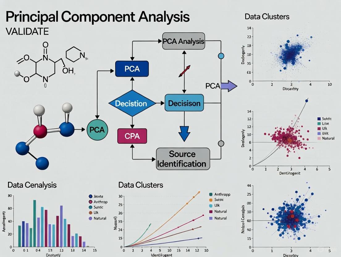
The following diagram illustrates the universal workflow of a source discrimination study, from sample analysis to final validation, which is applicable across both environmental and pharmaceutical contexts.

Comparative Experimental Data and Protocols

The application of PCA for source discrimination is demonstrated effectively through specific case studies in food safety, traditional medicine, and environmental monitoring. The quantitative outcomes from these distinct fields are summarized in the table below for direct comparison.

Table 1: Comparative Performance of PCA-Based Source Discrimination Methods

Field of Application	Analytical Technique	PCA Variant	Key Discriminatory Variables	Performance Outcome	Reference
Food Safety (Flour)	Near-Infrared (NIR) Spectroscopy	Comparative PCA (cPCA)	Spectral profiles of talcum powder	0.3% adulteration detection rate; eliminated brand-related background factors	[1]
Traditional Medicine (Poria)	Raman Spectroscopy	Multi-matrix Projection PCA	Molecular fingerprint (polysaccharides, triterpenoids)	97.5% accuracy in geographical origin identification	[2]
Environmental Science (Estuaries)	FTIR & Fluorescence Spectroscopy	PCA-APCS-MLR Receptor Model	Functional group composition (e.g., terrestrial, synthetic OM)	>85% compositional variance captured; validated against water quality data	[3]

Detailed Experimental Protocols

1. Flour Adulteration Identification via NIR and cPCA This protocol is designed to detect minute, deliberate contamination in food products.

• Sample Preparation: Obtain pure flour samples from different brands. Create adulterated samples by mixing pure flour with talcum powder at known, varying concentrations (e.g., from 0.1% to 5% by weight). Ensure homogeneous mixing.
• Spectral Acquisition: Use a NIR spectrometer to collect spectral data from each sample. A minimum of 20 spectral replicates per concentration level is recommended to ensure statistical robustness [1].
• Data Pre-processing: Apply standard spectral pre-processing techniques such as Standard Normal Variate (SNV) or multiplicative scatter correction to remove physical light-scattering effects and enhance chemical-based spectral features.
• cPCA Modeling: Implement the comparative PCA algorithm. This involves defining a "background" dataset (e.g., spectra from different flour brands) that the model will learn to ignore. The cPCA then effectively focuses on the variance specifically related to the adulterant, dramatically improving sensitivity and allowing detection at levels as low as 0.3% [1].

2. Geographical Origin Tracing of Poria via Raman and Multi-Matrix PCA This protocol provides a non-destructive method for authenticating the origin of high-value medicinal herbs.

• Sample Collection & Preparation: Source authenticated Poria cocos samples from distinct geographical origins (e.g., Yunnan, Anhui, Shaanxi, Hubei). The samples should be prepared as powders to ensure consistent spectral acquisition.
• Raman Spectroscopy: Use a 785 nm laser excitation Raman spectrometer. Acquire multiple Raman spectra (e.g., 25 spectra per origin) to build a robust training dataset. Reserve an independent set of spectra (e.g., 10 per origin) for model testing [2].
• Multi-Matrix Projection Discrimination:
  • Step 1: Perform PCA separately on the spectral dataset from each geographical origin. This generates a unique eigenvector matrix (a spectral "fingerprint") for each origin.
  • Step 2: For each test spectrum, project it onto all four origin-specific eigenvector matrices, creating four different reconstructed spectra.
  • Step 3: Calculate the Euclidean distance between the original test spectrum and each of its four reconstructions. The geographical origin is assigned based on the reconstruction with the smallest Euclidean distance, indicating the best fit [2].

3. Estuarine Sediment Source Apportionment via Multi-Spectroscopy and PCA-APCS-MLR This protocol is critical for identifying pollution sources in complex aquatic ecosystems.

• Field Sampling & Extraction: Collect surface sediment samples from various points in an estuary with contrasting land use. In the lab, extract the Water Extractable Organic Matter (WEOM) from each sediment sample.
• Multi-Spectroscopic Analysis:
  • FTIR Spectroscopy: Acquire infrared spectra of the WEOM. Develop and validate novel Infrared-Based Indices (IRIs) designed to be sensitive to functional groups from terrestrial, synthetic, and petroleum-derived organic matter [3].
  • Fluorescence Spectroscopy: Collect fluorescence excitation-emission matrices (EEMs) of the same extracts to gain complementary information on dissolved organic matter composition.
• Receptor Modeling: Integrate the spectroscopic data using the PCA-APCS-MLR model. The PCA reduces the multi-spectral data to a few key components. The Absolute Principal Component Scores (APCS) are used to estimate the contribution of each identified source (e.g., anthropogenic vs. natural) to the total sediment organic matter, with the Multiple Linear Regression (MLR) step quantifying their respective contributions [3].

The Scientist's Toolkit: Essential Reagents and Materials

Successful implementation of source discrimination studies relies on a set of key reagents, materials, and software tools.

Table 2: Essential Research Toolkit for Source Discrimination Studies

Tool Category	Specific Item / Technique	Primary Function in Source Discrimination
Analytical Instruments	Near-Infrared (NIR) Spectrometer	Rapid, non-destructive profiling of chemical composition in solids and liquids [1].
	Raman Spectrometer	Provides molecular fingerprint data based on vibrational modes; ideal for non-destructive analysis [2].
	Fourier-Transform Infrared (FTIR) Spectrometer	Identifies functional groups and organic compounds in environmental and material samples [3].
	Mass Spectrometer (e.g., LC-MS, FT-ICR-MS)	Provides definitive identification and quantification of individual compounds; used for model validation [3].
Chemometric Software	PCA & Comparative PCA (cPCA)	Core algorithm for dimensionality reduction and isolating target variance from complex backgrounds [1].
	PCA-APCS-MLR Receptor Model	A hybrid model that apportions contributions from multiple sources to a mixture [3].
Experimental Design	Design of Experiments (DoE)	A systematic, statistical approach for optimizing analytical methods and evaluating their robustness [4] [5].
Reference Materials	Authenticated Geographical Samples	Crucial for building and validating classification models for product origin [2].
	Analytical Grade Solvents	Essential for sample preparation and extraction without introducing contaminating signals.

The comparative data and methodologies presented in this guide unequivocally demonstrate that PCA-based statistical frameworks are indispensable for robust source discrimination. From ensuring food and pharmaceutical authenticity to apportioning environmental pollution, these techniques transform complex analytical data into actionable, validated insights. The consistent success of methods like cPCA and multi-matrix projection across diverse fields underscores their power and versatility, providing researchers and regulators with a reliable means to validate natural and anthropogenic source contributions.

A critical challenge across scientific disciplines is untangling mixed signals from multiple sources. In environmental science, this means distinguishing human-made (anthropogenic) pollution from naturally occurring (geogenic) elements; in pharmacology, it involves separating a drug's therapeutic effects from background biological noise. Principal Component Analysis (PCA) is a powerful, unsupervised multivariate statistical technique designed specifically for this task of dimensionality reduction and source identification. It works by transforming a large set of correlated variables into a smaller, more manageable set of uncorrelated variables called Principal Components (PCs), which capture the most significant patterns and variances in the data [6] [7]. This transformation allows researchers to visualize complex datasets, identify hidden structures, and apportion observed effects to their underlying sources, making it an indispensable tool for validating anthropogenic versus natural contributions in complex systems.

The core objective of PCA is to distill high-dimensional data into its essential features without significant loss of information. This process reveals the dominant patterns of variance, where the first principal component (PC1) captures the direction of maximum variance in the dataset, and each subsequent component captures the next highest variance under the constraint of being orthogonal to preceding components [6]. By analyzing which original variables contribute most heavily to each component, researchers can infer the distinct processes or sources—such as industrial emissions, volcanic activity, or specific biological pathways—that generate these characteristic patterns within the data [8].

Fundamental Principles of PCA

Mathematical Foundation and Workflow

Principal Component Analysis operates on a fundamental principle of linear algebra, transforming original variables into a new coordinate system. The mathematical procedure begins with the covariance matrix (or correlation matrix for standardized data), which expresses the relationships between all pairs of variables in the dataset [9]. The algorithm then performs an eigen decomposition of this matrix, calculating the eigenvectors (which define the directions of the new component axes) and eigenvalues (which represent the amount of variance explained by each component) [9]. The resulting principal components are linear combinations of the original variables, weighted by their contributions to each pattern of variance [10].

The standard workflow for implementing PCA follows a structured sequence: (1) Data Standardization - transforming variables to have zero mean and unit variance to prevent dominance by variables with larger scales; (2) Covariance Matrix Computation - calculating how variables vary together; (3) Eigenvalue Decomposition - extracting eigenvectors and eigenvalues; (4) Component Selection - choosing the number of components to retain based on variance explanation; (5) Interpretation - analyzing component loadings to infer meaningful patterns and sources [8]. This systematic approach ensures that the resulting components capture the most significant, independent sources of variation in the dataset.

Key Distinctions from Related Methods

PCA is often confused with Factor Analysis (FA), as both are dimension-reduction techniques, but they possess fundamental philosophical and mathematical differences. PCA creates new variables (components) as linear combinations of the original measured variables, with the goal of explaining maximum total variance in the data. In contrast, Factor Analysis posits latent variables (factors) that are assumed to cause the observed patterns in the measured variables, distinguishing between common variance (shared across variables) and unique variance (specific to each variable plus error) [10]. This distinction becomes crucial when selecting the appropriate method for source identification, with PCA generally being preferred for data reduction and pattern recognition, while FA is more suited for testing theoretical models of underlying constructs.

Beyond FA, PCA also differs from other ordination methods like Principal Coordinate Analysis (PCoA) and Non-Metric Multidimensional Scaling (NMDS). While PCA operates directly on the original data matrix (typically using Euclidean distance), PCoA starts with a distance matrix and can accommodate various distance measures, making it more flexible for ecological community data [6]. NMDS further differs by preserving only the rank-order of dissimilarities between samples, making it suitable for non-linear relationships [6]. The table below summarizes these key distinctions:

Table: Comparison of Multivariate Dimension Reduction Techniques

Characteristic	PCA	PCoA	NMDS	Factor Analysis
Input Data	Original feature matrix	Distance matrix	Distance matrix	Original feature matrix
Distance Measure	Covariance/Correlation matrix	Any distance measure	Any distance measure	Covariance/Correlation matrix
Variance Model	Explains total variance	Preserves relative distances	Preserves rank-order	Distinguishes common & unique variance
Primary Strength	Optimal variance capture	Flexible distance measures	Handles non-linear relationships	Models theoretical constructs
Typical Applications	Feature extraction, source identification	Ecological diversity, microbiome studies	Complex ecological communities	Psychology, social sciences

Comparative Performance of PCA

PCA Versus Clustering and Other Statistical Methods

The performance advantages of PCA become evident when compared to alternative statistical approaches like clustering algorithms. In a large-scale neuroimaging study comparing PCA with K-means clustering on identical data from 2,436 participants, PCA demonstrated superior goodness of fit when predicting diagnosis and body mass index (BMI) [11]. The study found that clustering methods artificially categorized continuous variables like age and BMI, while PCA more naturally represented the continuous gradients inherent in biological systems [11]. This advantage is particularly important when analyzing complex systems where boundaries between groups are ambiguous and variation occurs along spectra rather than discrete categories.

The performance of PCA also varies significantly depending on the analytical context, particularly in genetic association studies. Research has revealed that in SNP-set settings (testing multiple genetic variants against a single outcome), principal components with large eigenvalues tend to provide highest power, whereas in multiple phenotype settings (testing a single variant against multiple outcomes), higher-order components with smaller eigenvalues often yield better performance [12]. This counterintuitive finding highlights the importance of understanding context-specific PCA properties rather than applying the method generically across different study designs.

Application-Specific Performance Metrics

The effectiveness of PCA can be quantified through application-specific performance metrics across diverse fields. In financial portfolio risk analysis, PCA implementation improved risk assessment model accuracy from an adjusted R² of 0.62 to 0.88, while reducing portfolio risk exposure by 3.4% through more informed asset selection [13]. The correlation between PCA-extracted factors and portfolio performance increased from 0.82 to 0.88 over a four-year period, demonstrating its growing predictive alignment with market dynamics [13].

In process performance evaluation for manufacturing, PCA-based capability indices enabled robust assessment of multivariate process data without requiring the often-violated assumption of multivariate normality [7]. By transforming correlated quality characteristics into independent components, PCA provided accurate process capability metrics that would be unreliable using traditional multivariate methods, particularly for non-normal data distributions [7]. This flexibility across data types and structures further underscores PCA's utility as a robust analytical tool.

Table: Quantitative Performance Improvements Using PCA Across Disciplines

Field/Application	Performance Metric	Without PCA	With PCA	Improvement
Financial Risk Analysis	Model Accuracy (Adj. R²)	0.62	0.88	+42%
Financial Risk Analysis	Portfolio Risk Exposure	Baseline	-3.4%	Risk Reduction
Genetic Studies	Statistical Power	Varies by component	Optimal component selection	Context-dependent
Neuroimaging	Goodness of Fit (vs. Clustering)	Lower for clustering	Superior for PCA	Better clinical correlation
Process Manufacturing	Data Distribution Assumptions	Multivariate normal required	No distribution assumption	Greater robustness

Experimental Protocols for PCA Implementation

Standardized Workflow for Environmental Source Apportionment

A robust PCA protocol for environmental source identification requires meticulous data preparation and analytical standardization. A comprehensive study analyzing over 7,000 topsoil samples in Southern Italy established a standardized workflow that begins with Normal Score Transformation (NST) to stabilize variance and handle extreme outliers [8]. This preprocessing step pulls extreme values back toward normal ranges, creating a more suitable dataset for multivariate analysis without losing the meaningful information contained in outliers [8]. The transformed data then undergoes PCA with Varimax rotation, which maximizes the simplicity of the factor structure by enhancing the separation of variable loadings onto components, making interpretation more straightforward [8].

The experimental protocol continues with the spatialization of component scores, mapping them geographically to identify spatial patterns associated with different contamination sources [8]. In the Campania case study, this approach successfully discriminated between four primary independent sources controlling geochemical variability: two distinct volcanic districts, a siliciclastic component, and an anthropogenic component [8]. The integration of RGB composite maps further refined this differentiation by visualizing the coexistence and relative predominance of each source component across the region [8]. This comprehensive protocol provides a reproducible framework for environmental source apportionment in complex, anthropized regions.

Diagram: Experimental Workflow for PCA-Based Source Apportionment

Protocol for Molecular Dynamics Analysis in Drug Discovery

In drug discovery, PCA provides crucial insights into protein dynamics and ligand interactions that simpler metrics like RMSD (Root Mean Square Deviation) cannot capture. The standard protocol begins with Molecular Dynamics (MD) simulations of protein-ligand complexes, typically running for 50-200 nanoseconds to adequately sample conformational space [9]. The atomic coordinates from trajectory frames are then used to construct a 3N × 3N covariance matrix, where N represents the number of atoms analyzed [9]. Diagonalization of this matrix produces eigenvalues (representing the variance along each collective coordinate) and eigenvectors (the principal components themselves), which are sorted in descending order of explained variance [9].

The analytical phase involves projecting the original trajectories onto the first two or three principal components to create 2D or 3D maps of conformational space [9]. These projections reveal distinct protein conformational states and transitions that might be obscured in conventional analyses. For example, a PCA might reveal that a protein samples three distinct macrostates during a simulation, while RMSD analysis of the same data suggests only a single, stable conformation [9]. This capability makes PCA particularly valuable for identifying allosteric effects and understanding how different ligand modifications influence protein flexibility and binding site geometry in Free Energy Perturbation (FEP) studies [9].

Essential Research Toolkit for PCA Implementation

Software and Computational Tools

Successful PCA implementation requires appropriate computational tools tailored to specific research domains. For general statistical analysis, platforms like R (with packages like FactoMineR, factoextra, and prcomp), Python (with scikit-learn, pandas, and NumPy), and MATLAB provide robust, flexible environments for PCA computation and visualization [9]. Specialized software includes MDAnalysis for molecular dynamics trajectories [9], Flare for drug discovery applications [9], and IMSL (International Mathematics and Statistics Library) for manufacturing process capability analysis [7].

Many commercial statistical packages like SPSS, SAS, and JMP offer user-friendly PCA implementations with comprehensive visualization options, making the technique accessible to non-programmers [10]. The choice of software often depends on the scale of data, need for customization, integration with existing workflows, and domain-specific requirements. For extremely large datasets (e.g., genomic data), computational efficiency becomes a critical consideration, with some methods exhibiting complexity of O(n²d) for n samples and d dimensions [6].

Domain-Specific Reagents and Materials

The experimental inputs for PCA vary significantly across application domains, though all share the common requirement of high-quality, multidimensional data. The table below details essential "research reagents" and materials required for PCA across different fields:

Table: Essential Research Reagents and Materials for PCA Across Disciplines

Field	Essential "Reagents"/Inputs	Function in PCA Workflow	Technical Specifications
Environmental Science	Topsoil Samples	Primary source of geochemical data	Composite sampling, 100×100m grid [8]
	ICP-MS Analysis	Quantifies elemental composition	Measures heavy metals, trace elements [8]
	Normal Score Transformation	Preprocessing for skewed data	Stabilizes variance, handles outliers [8]
Drug Discovery	Molecular Dynamics Trajectories	Raw protein-ligand coordinate data	50-200ns simulation, all-atom resolution [9]
	Crystal Structures	Reference conformations	High-resolution (<2.5Å) protein-ligand complexes [9]
	MDAnalysis Toolkit	Trajectory analysis and PCA	Python package for MD analyses [9]
Neuroimaging	T1-Weighted MRI Scans	Cortical thickness measurements	Standardized protocols (ENIGMA) [11]
	Clinical/Demographic Data	Correlation with components	Diagnosis, medication, BMI, age [11]
Manufacturing	Product Quality Measurements	Multivariate process data	Multiple dimensions per unit (e.g., weight, dimensions) [7]
	Engineering Specifications	Tolerance limits for components	Upper/lower specification limits [7]

Diagram: Logical Relationships in PCA Workflow from Data to Interpretation

Case Studies in Source Validation

Mercury Pollution: Quantifying Natural vs. Anthropogenic Contributions

A compelling application of PCA in environmental source apportionment comes from research on atmospheric mercury at Canadian rural sites, where scientists combined long-term measurements with Positive Matrix Factorization (PMF) to quantify source contributions [14]. The study revealed that natural surface emissions dominated total gaseous mercury (TGM) at all three monitoring sites, accounting for 71-77.5% of annual TGM, while anthropogenic contributions showed consistent declining trends [14]. PCA-assisted analysis further delineated specific source types within these broad categories, identifying contributions from terrestrial re-emissions (24-26%), regional mercury emissions (11% at one site), oceanic re-emissions (6-8%), shipping emissions (10%), and local combustion (a few percent) [14].

This detailed source profiling enabled temporal analysis showing increasing contributions from natural surface Hg emissions (1.8% per year at one site) resulting from declining anthropogenic emissions and increasing oceanic re-emissions [14]. The study demonstrated striking seasonal patterns, with Hg pool contributions greater in cold seasons, while wildfire and surface re-emission contributions became more significant in warm seasons [14]. Such nuanced understanding of source dynamics would be impossible without PCA-based source apportionment, highlighting the technique's value in developing targeted environmental policies that address the most consequential emission sources.

Heavy Metal Contamination: Industrial Source Identification

In heavy metal contamination assessment, PCA enables precise identification of industrial sources through advanced statistical approaches. A study of soil heavy metals in Jiaozuo City, China, combined PCA with random forest models optimized by genetic algorithms to quantify specific influencing factors for pollution sources [15]. The analysis revealed three principal components representing distinct pollution sources with contribution rates of 47.2%, 33.3%, and 19.5%, respectively [15]. The first source was dominated by industrial activities, with factory density (27.7%) and distance from factory (36.3%) identified as the main factors, loading heavily with Cr, Cu, Mn, and Ni [15].

The second source represented a mixed natural/transportation influence, primarily affected by vegetation index (37.8%), road network density (16.8%), and proximity to roads (15.3%) [15]. The third source was linked to agricultural activities, with cultivated land density contributing 39.1% and As showing a high load (91.1%) [15]. This precise quantification of specific contributing factors moves beyond traditional source apportionment, which merely estimates percentage contributions of sources, providing instead a novel perspective for heavy metal source identification under complex environmental conditions [15].

Drug Discovery: Protein Conformational Analysis

In pharmaceutical research, PCA reveals subtle protein conformational changes induced by ligand binding that directly impact drug efficacy. Research has demonstrated that PCA of molecular dynamics trajectories can identify allosteric effects in dimeric proteins, where ligand binding at one site induces conformational changes at distant sites [9]. In one case study, PCA revealed that when only one binding site in a dimeric protein was occupied, the protein underwent significant restructuring, while occupancy of both sites resulted in a narrower conformational space closer to the initial structure [9]. This allosteric effect would have remained undetected using conventional analysis methods like RMSD.

PCA further supports drug discovery by identifying outlier compounds in congeneric series during Free Energy Perturbation (FEP) studies [9]. By projecting structures from FEP transformations onto PCA maps defined by reference simulations, researchers can quickly identify compounds that induce unusual protein conformations, potentially indicating undesirable binding modes or induced-fit effects [9]. This application allows medicinal chemists to prioritize compounds with optimal binding characteristics and understand the structural basis for energy predictions, ultimately accelerating the drug optimization process.

Principal Component Analysis stands as a versatile, powerful method for uncovering hidden source signatures across diverse scientific domains. Its mathematical foundation in covariance structure and eigen decomposition provides a robust framework for distilling complex, multivariate datasets into interpretable patterns that reveal underlying processes. The technique's demonstrated success in discriminating anthropogenic from natural contributions—whether in environmental mercury pollution, soil heavy metal contamination, or protein conformational changes—validates its essential role in source attribution studies.

As research datasets grow in dimensionality and complexity, PCA's importance as an analytical tool continues to increase. Future developments will likely focus on integration with machine learning approaches, enhanced computational efficiency for massive datasets, and improved visualization techniques for communicating complex multivariate relationships. The consistent performance of PCA across fields demonstrates its fundamental utility for researchers seeking to understand the hidden signatures embedded within their data, making it an indispensable component of the modern scientific toolkit.

Principal Component Analysis (PCA) is a powerful statistical technique for reducing the dimensionality of complex datasets, widely used to disentangle and quantify natural and anthropogenic pollution sources. This guide details the interpretation of core PCA outputs—loadings, scores, and variance—for accurate source identification, providing a structured comparison with alternative receptor modeling approaches.

Theoretical Foundations of PCA for Source Apportionment

Core Concepts and Definitions

Principal Component Analysis (PCA) is a dimensionality-reduction technique that transforms complex, high-volume datasets into a set of new, uncorrelated variables called principal components (PCs). These components are linear combinations of the original variables and are designed to successively maximize variance, thereby preserving as much statistical information as possible from the original data [16] [17]. The adaptability of PCA makes it particularly valuable for environmental forensics, where it helps identify underlying patterns in pollution data that signify different emission sources.

The technique operates by solving an eigenvalue/eigenvector problem derived from the covariance or correlation matrix of the original dataset [17]. In the context of source identification, each principal component potentially represents a distinct emission source or process, with the relative contributions of original chemical species to these components revealed through loadings, and the influence of this source across different samples revealed through scores [18] [19].

Mathematical Framework

Mathematically, PCA begins with a data matrix X containing observations on p numerical variables for each of n entities or samples. PCA seeks linear combinations of the columns of X with maximum variance, given by ( \mathbf{Xa} ), where a is a vector of constants [17]. The variance of such a linear combination is ( \text{var}(\mathbf{Xa}) = \mathbf{a'Sa} ), where S is the sample covariance matrix. Identifying the linear combination with maximum variance equates to finding a p-dimensional vector a that maximizes the quadratic form ( \mathbf{a'Sa} ) [17].

The solution to this optimization problem leads to the eigenvector equation: [ \mathbf{Sa} = \lambda\mathbf{a} ] where ( \lambda ) is a Lagrange multiplier and also an eigenvalue of the covariance matrix S [17]. The eigenvectors ak represent the PC loadings, while the projections of the original data onto these eigenvectors, ( \mathbf{Xa}k ), are the PC scores. The eigenvalues ( \lambdak ) represent the variances of the principal components, indicating how much variance each PC captures from the original dataset [18] [17].

Interpreting Key PCA Outputs for Source Identification

Loadings: Deciphering Source Profiles

PCA loadings, contained within the eigenvectors, are crucial for interpreting the meaning of each principal component in source identification studies. Loadings indicate the relative weight and direction of each original variable's contribution to a principal component [18]. In environmental source apportionment, each variable typically represents a specific chemical species or marker measured in the samples.

To interpret each principal component as a potential pollution source, researchers examine both the magnitude and direction (sign) of the loadings [18]. The larger the absolute value of a loading coefficient, the more important the corresponding variable is in calculating that component. For instance, in a study of PM2.5 sources, a component with high loadings for lead (Pb) and zinc (Zn) was interpreted as representing metals industry emissions, while a component with high loadings for elemental carbon (EC) and nitrogen dioxide (NO2) was identified as motor vehicle traffic [19]. The direction of the loadings indicates whether variables correlate positively (same direction) or negatively (opposite directions) within the component, potentially revealing complex source interactions or transformation processes.

Scores: Mapping Source Contributions

PCA scores represent the values that each individual sample would score on a given principal component [17]. These scores are calculated as linear combinations of the original data determined by the PC loadings [18]. In practical terms, scores indicate the relative contribution or influence of the source represented by a PC across different samples, locations, or time periods.

Scores can be visualized spatially to identify geographical patterns of source impacts or temporally to understand seasonal variations in source strength [19]. For example, in a nationwide PM2.5 source apportionment, plotting scores for a "biomass burning" component revealed highest impacts in the U.S. Northwest, while "residual oil combustion" showed elevated scores in Northeastern cities and major seaports [19]. Score plots also help identify outliers—samples with unusual source characteristics that may warrant further investigation [20].

Variance Explained: Determining Source Significance

The variance explained by each principal component indicates its importance in capturing the overall variability of the dataset. Eigenvalues represent the variances of the principal components, with larger eigenvalues indicating components that explain greater portions of the total variance [18]. The proportion of variance explained by each PC is calculated by dividing its eigenvalue by the total sum of all eigenvalues.

The cumulative proportion of variance explained by consecutive PCs guides researchers in deciding how many components (sources) to retain for interpretation [18]. As shown in Table 1, the first three principal components often explain the majority of variance in environmental datasets. The Kaiser criterion (retaining components with eigenvalues >1) provides a common retention threshold, though the adequacy of variance explained ultimately depends on the specific application [18].

Table 1: Representative Eigenanalysis Output for Source Identification Studies

Principal Component	Eigenvalue	Proportion	Cumulative Proportion
PC1	3.5476	0.443 (44.3%)	0.443 (44.3%)
PC2	2.1320	0.266 (26.6%)	0.710 (71.0%)
PC3	1.0447	0.131 (13.1%)	0.841 (84.1%)
PC4	0.5315	0.066 (6.6%)	0.907 (90.7%)
PC5	0.4112	0.051 (5.1%)	0.958 (95.8%)
PC6	0.1665	0.021 (2.1%)	0.979 (97.9%)
PC7	0.1254	0.016 (1.6%)	0.995 (99.5%)
PC8	0.0411	0.005 (0.5%)	1.000 (100.0%)

Source: Adapted from Minitab's PCA interpretation guide [18]

Comparative Analysis with Alternative Receptor Models

PCA vs. Absolute Principal Component Analysis (APCA)

While standard PCA identifies source profiles through loadings, it doesn't directly quantify mass contributions. Absolute Principal Component Analysis (APCA) extends PCA to provide quantitative source apportionment by scaling components using measured species concentrations [19]. In APCA, component scores are rescaled to represent absolute contributions to the total mass, enabling direct quantification of source impacts.

In a nationwide PM2.5 study, APCA was employed to quantify contributions from various sources after initial identification through standard PCA with varimax rotation [19]. This two-stage approach—using PCA for qualitative source identification followed by APCA for quantitative apportionment—provides a comprehensive framework for both understanding pollution sources and quantifying their contributions to ambient concentrations.

PCA-APCS-MLR: An Integrated Framework

The PCA-Absolute Principal Component Scores-Multiple Linear Regression (PCA-APCS-MLR) model represents a further refinement that integrates PCA with regression techniques for enhanced source quantification. This approach was successfully applied in a recent study deciphering natural and anthropogenic sources in estuarine sediment organic matter using multi-spectroscopic fingerprinting [3].

The PCA-APCS-MLR framework involves several stages: (1) PCA identifies potential sources and their profiles; (2) APCS calculates absolute component scores representing source contributions in each sample; and (3) MLR quantifies the relationship between source contributions and total mass, enabling precise apportionment. This integrated approach captured >85% of the compositional variance across all study sites, demonstrating its effectiveness for complex environmental systems [3].

Performance Comparison of Receptor Modeling Approaches

Table 2: Comparison of PCA-Based Receptor Models for Source Apportionment

Model Type	Key Features	Strengths	Limitations	Typical Applications
Standard PCA	Identifies source profiles through loadings; orthogonal components maximize variance [17]	No prior knowledge of sources required; reduces data dimensionality; visualizable through biplots [20]	Qualitative rather than quantitative; rotational ambiguity in interpretation	Initial exploratory analysis; hypothesis generation; identifying source types [19]
APCA	Extends PCA with absolute scoring for mass apportionment; uses measured species concentrations [19]	Quantitative mass apportionment; utilizes same statistical foundation as PCA	Requires measured mass data; sensitive to outliers and missing data	Quantifying source contributions to PM2.5 [19]; national-scale source apportionment
PCA-APCS-MLR	Integrated framework combining PCA, absolute scores, and multiple linear regression [3]	High explanatory power (>85% variance); quantitatively links sources to concentrations	Complex implementation; requires validation with independent datasets	Estuarine sediment sourcing [3]; complex environmental systems with mixed sources

Workflow and Methodological Protocols

Standardized PCA Protocol for Source Identification

The following workflow diagram illustrates the systematic approach for applying PCA in source identification studies:

PCA Workflow for Source Identification

Data Preparation and Standardization: The initial stage involves collecting and preparing the compositional data, typically including trace elements, ions, organic carbon (OC), elemental carbon (EC), and other source markers. Continuous variables should be standardized (mean-centered and scaled by standard deviation) to prevent variables with larger ranges from dominating the analysis [16]. In source apportionment studies, it's sometimes beneficial to exclude secondary components (sulfates, nitrates, organic carbon) from the initial PCA to more clearly discern primary emission sources, incorporating them later in mass apportionment [19].

Computational Core: The mathematical heart of PCA involves calculating the covariance or correlation matrix and performing eigendecomposition to extract eigenvalues and eigenvectors [17]. The covariance matrix captures how variables deviate from the mean together, revealing relationships between different chemical species that suggest common sources. Eigendecomposition transforms this matrix into eigenvectors (loadings) and eigenvalues (variances) that define the principal components [16] [17].

Interpretation and Validation: The final stage involves selecting meaningful components (often using Kaiser criterion of eigenvalue >1 or scree plot analysis), interpreting loadings to identify source profiles, and analyzing scores to understand spatial/temporal patterns of source impacts [18]. Validation may involve comparing PCA results with independent measurements or applying quantitative extensions like APCA or PCA-APCS-MLR for mass apportionment [19] [3].

Advanced Protocol: PCA-APCS-MLR for Quantitative Apportionment

For researchers requiring quantitative source contributions, the PCA-APCS-MLR protocol provides a comprehensive approach:

• Perform PCA on Standardized Data: Conduct PCA on the standardized dataset of compositional markers, retaining components with eigenvalues >1 [18] [3].

• Varimax Rotation: Apply varimax rotation to simplify the component structure, enhancing interpretability by maximizing high loadings and minimizing low ones.

• Calculate Absolute Principal Component Scores (APCS): Compute APCS by introducing a hypothetical "zero" sample and scaling the scores relative to this baseline, transforming them into absolute contributions [3].

• Multiple Linear Regression (MLR): Regress total measured mass concentrations against the APCS to obtain regression coefficients that represent the mass contribution of each source [3].

• Validation: Validate source contribution estimates using independent indicators, such as comparing modeled anthropogenic contributions with bottom water quality measurements in estuarine studies [3].

The Scientist's Toolkit: Essential Research Reagents and Materials

Table 3: Essential Research Reagents and Analytical Tools for PCA-Based Source Apportionment

Category	Specific Tools/Reagents	Function in Source Identification
Chemical Speciation Networks	U.S. EPA CSN (Chemical Speciation Network) data [19]	Provides standardized, nationwide PM2.5 composition data for multivariate analysis
Molecular Tracers	Fatty acids, fatty alcohols, saccharides, lignin and resin products, sterols [21]	Serve as molecular markers for specific sources (e.g., biomass burning, terrestrial organics)
Spectroscopic Tools	FTIR (Fourier Transform Infrared) spectroscopy, Fluorescence spectroscopy [3]	Provides fingerprinting capabilities for organic matter source discrimination
Statistical Software	R programming language, MATLAB, Minitab, SPSS, XLSTAT [16]	Performs PCA calculations, eigenvalue decomposition, and visualization
Validation Techniques	Ultrahigh-resolution mass spectrometry (FT-ICR-MS) [3]	Confirms chemical relevance of identified sources through molecular correlation
Ancillary Data	Bottom water quality datasets, meteorological data [3]	Provides independent validation of source contribution estimates

Application in Anthropogenic vs. Natural Source Discrimination

Case Study: Global Dust Emissions

PCA and related multivariate techniques have proven particularly valuable in quantifying the contributions of natural and anthropogenic dust sources across different climatic regions. A global simulation study revealed that while natural dust sources (primarily located in hyper-arid and arid regions like the Sahara and Arabian Desert) contributed 81.0% of global dust emissions, anthropogenic sources still accounted for a significant 19.0% [22]. This study demonstrated distinct spatial patterns: natural dust emissions dominated in arid regions with emission fluxes of 1-50 μg m⁻² s⁻¹, while anthropogenic dust emissions concentrated in semi-arid, sub-humid, and humid regions with generally lower fluxes of 0.1-10 μg m⁻² s⁻¹ [22].

The complex interplay between natural and anthropogenic sources was particularly evident in semi-arid regions, where mixed land cover types (grasslands, urban areas, croplands, open shrub lands) complicated simple discrimination. These regions accounted for 42.99% of global anthropogenic dust emissions, highlighting the importance of sophisticated statistical approaches like PCA for unraveling multiple source contributions in complex environments [22].

Case Study: Organic Aerosol Pollution in Urban Environments

In a comprehensive analysis of organic aerosols in Nanchang, Central China, receptor modeling approaches helped clarify the relative contributions of primary emissions and secondary formations to urban OA pollution. The results demonstrated that anthropogenic sources were the dominant determinant, contributing approximately 89% of primary organic carbon (POC) and primary organic aerosols (POA), and 60% of secondary organic carbon (SOC) and secondary organic aerosols (SOA) [21]. This clear discrimination between anthropogenic and natural influences, along with the quantification of primary versus secondary contributions, showcases the power of multivariate approaches in urban pollution studies.

Seasonal variations revealed further complexity: biogenic emissions exerted stronger influence during spring and summer, while anthropogenic emissions dominated in autumn and winter [21]. Such temporal patterns, identifiable through PCA score analysis, provide crucial information for targeted seasonal air quality management strategies.

Case Study: Estuarine Sediment Organic Matter

A recent innovative application of PCA-APCS-MLR successfully deciphered natural and anthropogenic sources in estuarine sediment organic matter across four South Korean estuaries with contrasting land use [3]. The study developed novel infrared-based indices (IRIs) from diagnostic FTIR absorbance features to capture source-specific functional group compositions linked to terrestrial, synthetic, and petroleum-derived organic matter.

The integrated framework, combining spectroscopic fingerprinting with receptor modeling, captured >85% of the compositional variance at all sites, providing a cost-effective alternative to more expensive molecular tools for routine source tracking in estuarine systems impacted by diverse anthropogenic pressures [3]. This approach demonstrates how PCA-based methods can be adapted and enhanced for specific environmental compartments and research questions.

The interpretation of PCA loadings, scores, and variance explained provides a robust foundation for identifying and apportioning pollution sources across diverse environmental contexts. When standard PCA is extended through approaches like APCA and PCA-APCS-MLR, it transitions from a qualitative exploratory tool to a quantitative method capable of discriminating between natural and anthropogenic contributions with high precision. The consistent application of these methods across global dust emissions, urban organic aerosols, and estuarine sediments demonstrates their versatility and effectiveness in addressing one of environmental science's most persistent challenges: reliably attributing pollution to its origins for more targeted and effective management.

In environmental and geochemical research, accurately distinguishing between anthropogenic (human-induced) and geogenic (naturally occurring) sources represents a fundamental challenge with significant implications for environmental risk assessment and remediation planning [8] [23]. The concept of "source end-members" refers to the definitive chemical profiles of pure contamination sources, which enable researchers to quantitatively apportion contributions from different sources in mixed environmental samples [24]. This distinction is particularly crucial in geochemically complex regions such as ore regions with historical mining activities, where naturally elevated concentrations of potentially toxic elements (PTEs) overlap with anthropogenic contamination [23]. Without robust methodological approaches to differentiate these sources, environmental assessments may misattribute contamination, leading to ineffective remediation strategies and misallocated resources.

Principal Component Analysis (PCA) has emerged as a powerful multivariate statistical technique for discerning patterns in complex environmental datasets and facilitating this critical distinction [8] [25]. By transforming correlated variables into a set of uncorrelated principal components, PCA captures the underlying structure of geochemical data, allowing researchers to identify distinct element groupings that reflect specific geochemical processes or sources [8]. This technical workflow provides a standardized, reproducible approach for characterizing anthropogenic and geogenic profiles across diverse environmental contexts, from soils and sediments to atmospheric particulate matter [8] [26].

Theoretical Framework and Key Concepts

Defining Geogenic and Anthropogenic End-Members

Geogenic sources derive from natural geological processes and exhibit chemical compositions reflecting local lithology, mineralogy, and weathering patterns. These natural backgrounds can be highly variable, with some regions exhibiting naturally elevated concentrations of potentially toxic elements due to geochemical haloes around mineralized zones [23]. In contrast, anthropogenic sources stem from human activities such as industrial production, mining, smelting operations, agricultural practices, and waste disposal, often introducing distinct chemical signatures into the environment [8] [23].

The fundamental principle of end-member mixing analysis leverages differences in chemical properties of environmental samples to quantify contributions from various sources without introducing man-made tracers [24]. This approach requires comprehensive characterization of potential source materials through detailed chemical analysis, recognizing that chemical compositions of end-members can vary both spatially and temporally [24]. In strongly anthropized regions, multiple independent sources often contribute to environmental contamination, requiring sophisticated statistical approaches to disentangle their respective contributions [8].

The Role of Principal Component Analysis in Source Discrimination

Principal Component Analysis serves as a dimensionality reduction technique that transforms correlated environmental variables into uncorrelated principal components, each representing linear combinations of original variables that capture maximum variance in the dataset [8]. The application of rotation methods such as Varimax produces a simpler structure, making it easier to associate element groupings with specific geochemical processes or sources [8]. The spatialization of PCA component scores can reveal primary independent sources controlling geochemical variability across a region, as demonstrated in the Campania region of Southern Italy where PCA successfully identified two distinct volcanic districts plus siliciclastic and anthropogenic components [8].

PCA applications in environmental geochemistry have proven particularly valuable for examining spatial distribution of elements in soils [8], discriminating contributions from different sources [25], and identifying key variables for environmental monitoring purposes [25]. The interpretability of PCA results depends heavily on appropriate data pre-treatment and understanding of local geological and anthropogenic contexts [25].

Analytical Approaches and Methodological Framework

Critical Constituents for End-Member Characterization

Robust end-member characterization requires analysis of comprehensive constituent groups that provide diagnostic information about potential sources. Based on extensive literature review of tracers useful for oil and gas activities and other industrial processes, the following constituent groups provide critical information for distinguishing anthropogenic and geogenic sources [24]:

Table 1: Key Analytical Constituents for End-Member Characterization

Constituent Group	Specific Parameters	Source Discrimination Utility
Dissolved Gases	Methane concentrations, carbon isotopic composition of methane (δ13C), hydrogen isotopic composition of methane (δ2H)	Distinguishes thermogenic (oil and gas sources) vs. biogenic (microbial processes) sources; identifies oxidation processes [24]
Major and Trace Elements	Major ions (Ca, Mg, Na, K, Cl, SO4), trace elements (As, Pb, Zn, Cu, Ti, Fe)	Element ratios (e.g., Pb/Ti, As/Fe) distinguish anthropogenic inputs from geogenic backgrounds; salinity sources [24] [23] [26]
Isotopic Tracers	Stable isotopes of water (δ2H, δ18O), dissolved carbon (δ13C), strontium (87Sr/86Sr), boron (δ11B), lithium (δ7Li)	Determine sources of water and salts; calculate groundwater ages; distinguish contamination sources [24]
Noble Gases	Helium (He), neon (Ne), argon (Ar) isotopic ratios	Identify atmospheric vs. deep subsurface sources; detect fluid injection impacts; determine recharge locations [24]
Organic Compounds	Volatile organic compounds (VOCs), polycyclic aromatic hydrocarbons (PAHs), dissolved organic carbon (DOC) fractions	Differentiate petroleum sources vs. other organic carbon sources; indicators of industrial activities [24]
Radioactive Elements	Radium (Ra), uranium (U) isotopes	Effective tracers of fluids from zones of oil and gas deposits; natural radioactive decay series [24]

Experimental Design and Sampling Strategies

Comprehensive end-member characterization requires strategic sampling approaches that account for both spatial and temporal variability:

Vertical Profiling: Comparative analysis of topsoils (0-20 cm) and subsoils (40-80 cm) enables discrimination between surface anthropogenic inputs and natural geogenic backgrounds [23]. Subsoils typically reflect local geochemical backgrounds, while topsoils integrate both geogenic and anthropogenic contributions, with their difference indicating anthropogenic contamination [23].

Reference Sampling: Collection of samples from known anthropogenic sources (industrial emissions, mining waste, agricultural runoff) and representative geological materials (bedrock, unweathered parent material) provides essential reference end-members [23].

Temporal Sampling: For atmospheric particulates or dynamic water systems, time-series sampling captures temporal variations in source contributions, essential for understanding seasonal patterns or response to specific events [26].

Density and Scale: High-density sampling across geological and anthropogenic gradients ensures adequate representation of spatial heterogeneity, particularly in geochemically complex areas [8] [23]. The Campania region study analyzed over 7000 topsoil samples across 13,600 km² to adequately characterize regional patterns [8].

Laboratory Analytical Methods

Advanced analytical techniques are required to measure the comprehensive suite of constituents necessary for end-member characterization:

Table 2: Essential Analytical Methods for End-Member Characterization

Analytical Technique	Measured Parameters	Application in Source Discrimination
ICP-MS/OES	Major and trace element concentrations	Elemental fingerprints for different source materials; calculation of element ratios [23]
Isotope Ratio Mass Spectrometry	Stable isotope ratios (C, H, O, Sr, B, Li)	Natural tracers of specific geological formations and anthropogenic processes [24]
Gas Chromatography with Combustion-IRMS	Carbon and hydrogen isotopic composition of methane	Distinguishes thermogenic vs. biogenic methane sources; identifies methane oxidation [24]
GC-MS	Volatile and semi-volatile organic compounds	Molecular markers for specific industrial activities or petroleum sources [24]
Gamma Spectrometry	Naturally occurring radioactive materials	Tracers for fluids from specific geological formations [24]
Ion Chromatography	Major anions and cations	Salinity sources; water-rock interaction indicators [24]

Data Pre-Treatment and Statistical Analysis

Data Pre-Treatment for PCA

Appropriate data pre-treatment is essential for meaningful PCA results, as different pre-treatment methods can significantly influence outputs and interpretation [25]:

Normalization Techniques: Geochemical data often exhibit non-normal distributions with outliers that can strongly influence statistical analysis [8]. Normal Score Transformation (NST) stabilizes variance in datasets, pulling extreme outliers back to normal ranges and making data more suitable for multivariate analysis [8]. Alternative approaches include Box-Cox transformation and log-transformation, though results can vary moderately between methods [8].

Grain Size Normalization: For sediment datasets, granulometric normalization reduces the overwhelming influence of grain size on metal variability, allowing other factors including mineralogy and anthropogenic sources to be identified more clearly [25].

Outlier Management: Identification and removal of outlying samples is critical, as a small number of high/low magnitude samples can create factors that do not represent the majority of the data [25]. Statistical approaches such as the use of correlation matrices rather than transformations can help reduce outlier influence [25].

Centering and Scaling: Performing PCA on a correlation matrix corrects for magnitude and scale differences between variables measured in different units [25]. The choice of data center (sample means vs. control group means) should align with experimental design objectives [27].

PCA Implementation and Interpretation

The PCA workflow involves multiple stages from data preparation to interpretation:

Component Selection: The number of meaningful components is determined through scree plot analysis, evaluating eigenvalues, and considering the percentage of variance explained [8]. In environmental applications, the first few components typically capture the major sources of variability, with subsequent components representing noise or minor influences [25].

Source Interpretation: Factor loadings indicate the correlation between original variables and principal components, revealing element associations that reflect specific geochemical processes or sources [8] [25]. For example, associations of Pb, Zn, and Cu typically indicate anthropogenic mining sources, while associations of Al, Ti, and Fe reflect natural lithogenic sources [23]. Factor scores indicate how strongly individual samples associate with each component, facilitating identification of samples with similar composition and potential sources [25].

Spatialization: Mapping PCA component scores across study areas reveals spatial patterns of source influences, highlighting areas dominated by specific anthropogenic or geogenic sources [8]. RGB composite maps of multiple component scores can further refine differentiation, emphasizing the coexistence or predominance of one component over another [8].

Case Studies and Applications

Distinguishing Mining Contamination in the Ore Mountains

In the Ore Mountains (Czech Republic), a region with extensive historical mining and smelting activities, researchers employed empirical cumulative distribution functions (ECDFs) to distinguish geogenic and anthropogenic contributions to soil contamination by As, Cu, Pb, and Zn [23]. The approach combined detailed topsoil and subsoil sampling with element ratio analysis (As/Fe, Pb/Ti) to account for natural variability in soil composition. The study found that local backgrounds for As/Fe and Pb/Ti were naturally elevated (5.7-9.8 times and 2.1-2.7 times higher than global averages, respectively) due to geochemical haloes around ore veins [23]. Through ECDF analysis, researchers quantified anthropogenic contributions as approximately 16% and 12% for As/Fe and 17% and 14% for Pb/Ti in the two study areas, corresponding to topsoil enrichment of approximately 15-14 mg kg⁻¹ for As and 35-42 mg kg⁻¹ for Pb [23].

Regional Geochemical Mapping in Campania, Italy

A large-scale study in Campania (Southern Italy) applied PCA to over 7000 topsoil samples across 13,600 km² to identify sources controlling geochemical variability [8]. The methodology applied Normal Score Transformation to stabilize variance before conducting PCA with Varimax rotation [8]. The spatialization of four selected component scores revealed four primary independent sources: two distinct volcanic districts, a siliciclastic component, and an anthropogenic component [8]. RGB composite maps further refined this differentiation, demonstrating the value of PCA for identifying regional-scale geochemical patterns in complex geological settings with significant anthropogenic pressure [8].

Atmospheric Particulate Source Apportionment in Beijing

A two-year sampling study of total suspended particles (TSP) in Beijing used element ratios (Pb/Ti) to distinguish between periods dominated by geogenic or anthropogenic pollution [26]. The research demonstrated that chemical composition combined with meteorological data could reflect specific influences of distinct aerosol sources, with considerable variation in source contributions over the course of the year [26]. The interactions between aerosols from different sources were numerous, highlighting the complexity of source apportionment in urban atmospheres with multiple contamination sources [26].

Advanced Techniques and Methodological Considerations

Uncertainty Assessment in PCA Results

The application of bootstrap methods such as the Truncated Total Bootstrap (TTB) procedure enables assessment of uncertainty in PCA results [28]. This approach simulates multiple "virtual panels" from original data to investigate uncertainty in paired comparisons between samples [28]. Accounting for mutual dependencies in bootstrap-derived results prevents misleading conclusions that can arise when treating results from the same virtual panel as independent data [28]. Visualization of uncertainty regions for each sample facilitates more robust interpretation of differences between anthropogenic and geogenic sources.

Element Ratios and Diffuse Contamination Assessment

Element ratios normalized to conservative lithogenic elements (e.g., Pb/Ti, As/Fe, Zn/Al) provide powerful tools for distinguishing anthropogenic contributions from natural geochemical variability [23] [26]. This approach accounts for natural variations in soil composition due to differences in mineralogy and texture [23]. The assessment of diffuse contamination—widespread low-level contamination often challenging to detect—is particularly facilitated by ECDF analysis of element ratios in topsoil and subsoil pairs [23]. This method enables identification of diffuse contamination through systematic shifts in ECDF curves that affect most samples in a dataset rather than creating distinct outliers [23].

Multi-Proxy Statistical Approaches

While PCA represents a powerful standalone technique, its effectiveness increases when integrated with complementary statistical approaches:

End-Member Mixing Analysis (EMMA): Chemical analyses of "end-member" samples enable quantification of each end-member's contribution to groundwater or soil samples, using differences in chemical properties without introducing man-made tracers [24].

Empirical Cumulative Distribution Functions (ECDFs): Comparison of ECDFs for potentially toxic elements and lithogenic elements in topsoils and subsoils facilitates distinction between natural topsoil enrichment, point contamination, and diffuse contamination [23].

Cluster Analysis: Combined with PCA, cluster analysis identifies groups of samples with similar chemical composition, potentially representing areas influenced by similar sources [28].

Research Reagent Solutions and Essential Materials

Table 3: Essential Research Reagents and Materials for End-Member Characterization

Category	Specific Items	Application and Function
Field Sampling	Stainless steel trowels, grab samplers, soil corers, GPS units	Collection of representative soil/sediment samples with accurate spatial referencing [25]
Sample Preservation	Chemical-grade acids, sterile containers, temperature-controlled storage	Preservation of sample integrity between collection and analysis [24]
Laboratory Analysis	ICP-MS/OES calibration standards, isotope reference materials, chromatography supplies	Quality assurance/quality control for analytical measurements [24] [23]
Data Analysis	Statistical software with multivariate analysis capabilities (R, SPSS, Statistica)	Implementation of PCA and complementary statistical techniques [8] [25]
Geospatial Analysis	GIS software, spatial interpolation tools	Spatialization of PCA results and mapping of source contributions [8]

The characterization of anthropogenic and geogenic source end-members through Principal Component Analysis and complementary statistical techniques provides a robust framework for environmental source apportionment in complex systems. The methodological workflow encompassing appropriate sampling design, comprehensive chemical analysis, careful data pre-treatment, and informed statistical interpretation enables researchers to distinguish between natural and human-derived contamination even in geochemically anomalous settings. The integration of element ratios, spatial analysis, and uncertainty assessment further strengthens these approaches, providing environmental managers with scientifically-defensible basis for remediation decisions and risk assessments. As analytical capabilities continue to advance and statistical methods become more sophisticated, the precision and reliability of source end-member characterization will continue to improve, supporting more effective environmental management in increasingly complex anthropized landscapes.

Principal Component Analysis (PCA) is a powerful statistical technique for simplifying complex, high-dimensional datasets. By transforming numerous correlated variables into a smaller set of uncorrelated principal components, PCA reveals underlying patterns and structures that are critical for interpreting real-world phenomena. This guide explores how PCA is applied to distinguish between natural and human-made sources of contamination in environmental science and to analyze high-dimensional data in drug discovery, providing a direct comparison of its performance against other dimensionality reduction methods.

A primary application of PCA in environmental science is identifying the origin of pollutants in soil and groundwater, which is a crucial first step for effective remediation and policy-making.

Case Study 1: Topsoil Contamination in Southern Italy

A 2025 study analyzed over 7,000 topsoil samples across the Campania region to determine the sources of geochemical elements [8].

• Experimental Protocol: Researchers collected topsoil samples based on methodologies from the EuroGeoSurveys geochemical mapping program [8]. The area was divided into a 100x100 m grid, and composite samples were created for each site for representativeness [8]. The key methodological steps are outlined below:

• Key Findings and Source Discrimination: The PCA successfully isolated four independent sources controlling the region's geochemistry [8]. The subsequent spatial analysis mapped these components, revealing their geographic predominance and co-existence [8]. The results are summarized in the following table:

Principal Component	Identified Source Type	Key Characteristics / Elements
Component 1	Volcanic District 1	Associated with the Somma-Vesuvius volcanic system [8].
Component 2	Volcanic District 2	Associated with the Phlegraean Fields volcanic system [8].
Component 3	Siliciclastic Geology	Derived from sedimentary rocks like siltstones and sandstones in hilly regions [8].
Component 4	Anthropogenic Activity	Linked to urban, industrial, and agricultural inputs [8].

Case Study 2: Groundwater Radioactivity and Nitrates in Southern Tunisia

A study of 33 groundwater samples from the Gafsa basin used PCA to differentiate sources of radioactive and nitrate contamination [29].

• Experimental Protocol: The study area is known for phosphate mining and agriculture [29]. Researchers collected groundwater samples and analyzed them for radioactive isotopes (e.g., radium) and nitrate concentrations [29]. The resulting data matrix was processed through PCA without specific normalization mentioned in the abstract [29].
• Key Findings and Source Discrimination: PCA classified the samples into distinct groups based on contamination origin [29]. The analysis revealed that samples most impacted by human activity showed high concurrent levels of radium and nitrates [29].

Contamination Source	Key Contributing Activities	Impact on Groundwater
Phosphate Mining	Extraction and processing of phosphate rock.	Primary source of radioactivity (e.g., radium) [29].
Agricultural Runoff	Use of fertilizers and manures on crops.	Major source of nitrate (NO₃⁻) contamination [29].
Fossil Geothermal Waters	Natural deep groundwater upwelling.	Contributed to radioactivity from the North Western Sahara Aquifer System [29].

Case Study 3: Groundwater Quality in Ho Chi Minh City, Vietnam

A study analyzing 233 well-water samples in 2015 and 20 in 2019 used PCA/FA (Factor Analysis) to apportion pollution sources [30].

• Experimental Protocol: Water samples were analyzed for key parameters. In 2015, 8 parameters were measured, expanding to 15 in 2019 [30]. PCA/FA was applied to the dataset to identify latent factors representing different pollution sources.
• Key Findings and Source Discrimination: The analysis identified three major pollution sources, ranking them in order of importance: agricultural, urban, and industrial activities [30]. The Groundwater Quality Index (GQI) showed that water quality ranged from poor to very poor, with the agricultural area being the most severely degraded [30].

Health Sciences Case Study: Analyzing Drug-Induced Transcriptomic Data

Beyond environmental science, PCA is a foundational tool for analyzing high-dimensional data in health research, though it is often benchmarked against newer algorithms.

Case Study: Benchmarking Dimensionality Reduction for Drug Response

A 2025 study systematically evaluated 30 different dimensionality reduction (DR) methods, including PCA, on their ability to preserve biological information in drug-induced transcriptomic data from the Connectivity Map (CMap) dataset [31].

• Experimental Protocol: The benchmark used 2,166 drug-induced transcriptomic profiles from nine cell lines [31]. DR methods were tested under four conditions to evaluate their ability to preserve biological similarity [31]:
  • Different cell lines treated with the same drug.
  • Same cell line treated with different drugs.
  • Same cell line treated with drugs having different Mechanisms of Action (MOAs).
  • Same cell line treated with varying dosages of the same drug.
• Performance Metrics: Methods were evaluated using internal validation metrics (Davies-Bouldin Index, Silhouette score) and external validation metrics (Normalized Mutual Information, Adjusted Rand Index) that measured how well the low-dimensional embeddings agreed with known biological labels [31].

Performance Comparison of Dimensionality Reduction Methods

The benchmarking study provided a direct, data-driven comparison of PCA's performance against modern alternatives like UMAP and t-SNE [31].

Dimensionality Reduction Method	Key Algorithmic Principle	Performance in Preserving Biological Structure	Suitability for Drug Response Data
PCA (Principal Component Analysis)	Identifies directions of maximal variance; linear transformation.	Relatively poor in preserving local biological similarity and cluster compactness compared to top performers [31].	Good for global structure and interpretability; may obscure finer, local differences crucial for distinguishing drug MOAs [31].
t-SNE (t-Distributed Stochastic Neighbor Embedding)	Minimizes divergence between high- and low-dimensional similarities; emphasizes local neighborhoods.	Top performer in separating distinct drug responses and grouping drugs with similar MOAs [31].	Well-suited for capturing local cluster structures; effective for discrete drug responses [31].
UMAP (Uniform Manifold Approximation and Projection)	Uses cross-entropy loss to balance local and global structure.	Top performer, comparable to t-SNE, with strong cluster separability [31].	Offers improved global coherence; well-suited for studying discrete drug responses [31].
PaCMAP (Pairwise Controlled Manifold Approximation)	Incorporates distance-based constraints for local and global structure.	Top performer, consistently high rankings across internal and external validation metrics [31].	Effective at preserving both local detail and long-range relationships [31].
PHATE	Models diffusion-based geometry to reflect manifold continuity.	Stronger performance in detecting subtle dose-dependent transcriptomic changes [31].	Well-suited for datasets with gradual biological transitions, such as dose-response curves [31].

The study concluded that while t-SNE, UMAP, and PaCMAP are excellent for studying discrete drug responses (e.g., different MOAs), most methods, including PCA, struggled with subtle dose-dependent changes, an area where Spectral methods and PHATE showed more strength [31]. A key finding was that PCA's widespread use is not supported by top-tier performance in this biological context, as it was outperformed by multiple non-linear techniques [31].

The Researcher's Toolkit for PCA-Based Studies

The following table details essential reagents, software, and methodological components for conducting PCA in environmental and health studies.

Tool / Material	Function / Role in PCA Workflow
Geochemical Soil Samples	Primary environmental matrix for analyzing elemental concentrations and identifying geogenic vs. anthropogenic sources [8].
Groundwater Samples	Primary environmental matrix for measuring chemical and radioactive contaminants to apportion pollution sources [29] [30].
Cell Lines (e.g., A549, MCF7)	In vitro model systems used to generate drug-induced transcriptomic data for pharmacological analysis [31].
Normal Score Transformation (NST)	A normalization technique that stabilizes variance in skewed geochemical data, pulling extreme outliers back to normal ranges for more robust multivariate analysis [8].
Varimax Rotation	An orthogonal rotation method used in PCA to simplify the factor structure, making it easier to associate element groupings with specific processes or sources [8].
Connectivity Map (CMap) Dataset	A comprehensive public resource of drug-induced transcriptomic profiles used as a benchmark for evaluating analytical methods in drug discovery [31].
Internal Validation Metrics (DBI, Silhouette)	Metrics like the Davies-Bouldin Index (DBI) and Silhouette score that assess cluster compactness and separation without external labels, used to evaluate DR method quality [31].

The case studies demonstrate that PCA is a versatile and powerful method for source apportionment in environmental science, effectively distinguishing between natural geological signals and anthropogenic pollution in soil and water [8] [29] [30]. However, in the analysis of highly complex biological data like drug-induced transcriptomics, its performance is surpassed by modern non-linear dimensionality reduction techniques such as t-SNE, UMAP, and PaCMAP [31]. The choice of method should be guided by the data's nature and the research question—whether it requires capturing global variance (PCA) or intricate local structures (UMAP, t-SNE) [31].

From Theory to Practice: A Step-by-Step PCA Workflow for Source Validation

In environmental forensics and geochemical research, reliably differentiating between anthropogenic pollution and natural background sources is a fundamental challenge with significant implications for environmental risk assessment and remediation planning [8] [32]. Principal Component Analysis (PCA) has emerged as a powerful multivariate statistical technique for contaminant source attribution, capable of discerning patterns in complex environmental datasets by transforming correlated variables into a set of uncorrelated principal components that capture underlying data structure [33] [25]. However, the reliability of PCA outputs is profoundly dependent on strategic data collection and rigorous preprocessing methodologies implemented during this initial phase. The integrity of conclusions regarding anthropogenic versus natural contributions hinges entirely on these foundational steps, which must be carefully designed to address the unique challenges of environmental data, including non-normal distributions, outliers, grain size effects, and multiple confounding factors [8] [25].

Strategic Sampling Design and Data Collection Protocols

Sampling Framework and Spatial Design

Effective sampling strategies for source apportionment studies employ systematic approaches that capture both the spatial variability and potential contaminant hotspots. Research on topsoil geochemical patterns in strongly anthropized regions demonstrates the value of comprehensive sampling networks, with studies analyzing over 7,000 samples across approximately 13,600 km² to adequately characterize regional variability [8]. Sampling designs should incorporate:

• Grid-based sampling: Implementing systematic 100×100 m grids or similar regular sampling nodes ensures comprehensive spatial coverage and avoids sampling bias [8] [34].
• Background reference sites: Including control sites with no known anthropogenic influence provides crucial baseline data for distinguishing natural background concentrations [32] [34].
• Source-proximate sampling: Collecting samples near potential anthropogenic sources (industrial facilities, roadways, agricultural areas) helps characterize source signatures [35].
• Stratified approaches: Dividing study areas based on geological features, land use, or population density ensures representative coverage of different environmental compartments [34].

Sample Collection and Handling Protocols

Standardized field protocols are essential for generating comparable, high-quality data. Key methodological considerations include:

• Composite sampling: Mixing subsamples from multiple points within a sampling site increases representativeness and reduces local variability [8].
• Consistent depth sampling: For soil studies, collecting surface samples at standardized depths (e.g., 5-cm depth after removing plant debris) ensures comparability [34].
• Contamination prevention: Using sterile containers and clean sampling equipment prevents cross-contamination [34].
• Metadata documentation: Recording precise coordinates, soil characteristics, land use, and environmental conditions provides essential context for interpreting analytical results [34].

Table 1: Key Environmental Compartments and Sampling Considerations for Source Apportionment Studies

Environmental Compartment	Sampling Protocol	Key Parameters	Special Considerations
Topsoil	Composite samples from standardized depth (0-5 cm); 100×100 m grid	Heavy metals, PAHs, PFAS, major elements	Remove plant debris; consider seasonal variability
Sediments	Surface scrapes (intertidal) and grab samplers (subtidal)	Grain size, metals, organic content, TOC	Grain size normalization critical for interpretation
Ambient PM2.5	24-hour sampling on filter media with portable sampler	Heavy metals, elemental carbon, ions	Consider wind direction; indoor/outdoor pairs
Groundwater	Monitoring wells; low-flow sampling	PFAS, solvents, metals, ions	Consider groundwater flow direction and seasonal fluctuations

Data Preprocessing and Normalization Methodologies

Addressing Data Distribution Challenges

Environmental data often exhibit non-normal distributions with significant skewness and outliers, requiring appropriate transformations before PCA application [8] [25]. Research demonstrates that different preprocessing approaches can significantly impact PCA interpretation and source attribution conclusions [25]:

• Normal Score Transformation (NST): Effectively stabilizes variance in datasets with extreme outliers, "pulling extreme outliers back to normal ranges" to create more robust datasets for multivariate analysis [8].
• Logarithmic transformation: Traditional log(x+1) transformation can skew negatively skewed data and mask important trends, making it less desirable than NST for many environmental datasets [25].
• Outlier treatment: Identifying and removing extreme outliers (e.g., through visual inspection of distribution histograms) prevents distortion of principal components, as "a small number of high/low magnitude samples can create factors that do not represent the main dataset" [25].

Covariate Normalization Techniques

Environmental covariates such as grain size in sediments or organic content in soils can dominate variance and obscure meaningful patterns related to contaminant sources. Effective normalization strategies include:

• Grain size normalization: For sedimentary environments, metals preferentially associate with fine-grained fractions due to greater surface area, requiring normalization to account for natural variability [32] [25]. Research shows that "granulometric normalisation meant that other factors affecting metal variability, including mineralogy, anthropogenic sources and distance along the salinity transect could be identified and interpreted more clearly" [25].
• Geochemical normalization: Using conservative elements such as aluminum (Al) or iron (Fe) as reference elements can help distinguish anthropogenic enrichments from natural mineralogical variations [32].
• Organic carbon normalization: For organic contaminants, normalizing to total organic carbon (TOC) content helps account for differential partitioning behavior.

Table 2: Comparison of Data Preprocessing Methods for Environmental PCA

Preprocessing Method	Applications	Advantages	Limitations
Normal Score Transformation	Skewed geochemical data with outliers	Stabilizes variance; handles extreme values effectively	Less familiar to some researchers; requires specialized software
Log Transformation	Traditionally used for right-skewed data	Simple to implement; widely understood	Can worsen negative skew; may mask important trends
Grain Size Normalization	Sediment metal concentrations	Reveals patterns obscured by sedimentological variability	Requires additional analytical data (%fines, Al content)
Geochemical Normalization	Distinguishing anthropogenic from natural elements	Uses conservative elements (Al, Fe) as mineralogical references	Assumes normalizing element is not anthropogenically enriched

The following workflow diagram illustrates the complete data collection and preprocessing pipeline for reliable PCA modeling:

Quality Assurance and Analytical Considerations

Analytical Method Selection and Validation

Selecting appropriate analytical methods with adequate sensitivity and specificity is crucial for generating reliable data. Research on heavy metals in PM2.5 demonstrates the importance of method detection limits that accommodate both background concentrations and potential anthropogenic enrichments [35]. Key considerations include:

• Detection limits: Ensuring method detection limits are sufficiently low to quantify background concentrations, especially for toxic elements of concern [34].
• Standard reference materials: Incorporating certified reference materials with similar matrices to evaluate analytical accuracy [34].
• Quality control samples: Including field blanks, duplicates, and spike recoveries to assess potential contamination and analytical precision [35].
• Multi-element techniques: Utilizing comprehensive analytical approaches like ICP-MS/AES that provide coordinated multi-element data essential for PCA [34] [35].

Data Quality Assessment Protocols

Before proceeding to multivariate analysis, systematic data quality assessment should include:

• Completeness evaluation: Assessing the percentage of missing data and implementing appropriate imputation strategies where justified.
• Precision assessment: Calculating relative percent difference between duplicate analyses to quantify analytical variability.
• Accuracy verification: Comparing results for certified reference materials to established values to identify potential analytical biases.
• Data distribution examination: Creating histograms and calculating skewness/kurtosis to inform appropriate transformation approaches [25].

Essential Research Reagent Solutions

Table 3: Key Research Reagents and Materials for Environmental Source Apportionment Studies

Reagent/Material	Application	Function	Technical Considerations
Sterile Whirl-Pak Bags	Soil sample collection & storage	Prevent cross-contamination during transport	Pre-sterilized; chemically inert
ICP-MS/Grade Acids	Sample digestion for metal analysis	Extract metals from solid matrices while maintaining ultra-pure conditions	High-purity nitric and hydrochloric acid
47 mm Glass Fiber Filters	PM2.5 sampling for airborne metals	Collect fine particulate matter with high efficiency	Compatible with MiniVol TAS-5.0 and similar samplers
Certified Reference Materials	Quality assurance for analytical accuracy	Verify method performance for specific matrices	Should match sample matrix (soil, sediment, etc.)
Quality Control Standards	Instrument calibration & continuing calibration verification	Ensure analytical precision and accuracy over time	Multi-element mixtures at relevant concentrations

Strategic data collection and meticulous preprocessing constitute the critical foundation for reliable PCA modeling in environmental source apportionment research. The methodologies outlined in this guide—from systematic sampling designs that adequately capture spatial variability to appropriate data normalization techniques that address fundamental geochemical principles—enable researchers to distinguish between anthropogenic and natural contributions with greater confidence. By implementing these rigorous approaches during Phase 1, environmental scientists create the necessary conditions for PCA to effectively reveal underlying source patterns rather than artifacts of sampling bias, analytical variance, or confounding environmental factors. These protocols transform raw environmental measurements into scientifically defensible data structures capable of supporting robust conclusions about contaminant origins, ultimately informing evidence-based environmental management decisions and remediation strategies.

Geochemical data are inherently compositional and typically exhibit strongly skewed distributions, presenting significant challenges for statistical analysis and interpretation [36]. The presence of outliers and non-normal distributions can profoundly influence the results of multivariate techniques like Principal Component Analysis (PCA), which is crucial for discriminating between anthropogenic and natural geochemical sources [8] [37]. Effective normalization and transformation of these skewed datasets represent an essential preprocessing step to ensure the reliability of environmental source apportionment studies. This guide provides a comprehensive comparison of current techniques, assessing their performance characteristics, computational requirements, and suitability for different geochemical contexts to support researchers in selecting optimal methodologies for their specific applications.

Fundamentals of Geochemical Data Distributions

Geochemical element concentrations rarely follow simple normal distributions in their raw form. Instead, they typically demonstrate complex distribution patterns including log-normal, power-law, and multimodal distributions resulting from multiple geological processes and anthropogenic influences [36]. These distribution characteristics arise from the fundamental nature of geochemical systems, where element concentrations are constrained by a constant sum (100%), creating what is known as closed data or compositional data [38] [39].

The skewed nature of geochemical data manifests through several measurable properties. Statistical parameters such as high skewness and kurtosis values provide quantitative evidence of distribution asymmetry and tailedness, while large coefficients of variation (CV > 1) indicate highly heterogeneous spatial distributions often associated with mineralization zones [40]. These distribution characteristics directly impact analytical outcomes, potentially leading to biased correlation estimates, spurious principal components, and ultimately, misinterpretation of geochemical sources when unaddressed through appropriate transformation techniques [8].

Normalization and Transformation Techniques: Comparative Analysis

Traditional Statistical Transformation Methods

Table 1: Comparison of Traditional Transformation Methods for Geochemical Data

Method	Mathematical Formulation	Key Advantages	Principal Limitations	Optimal Use Cases
Log Transformation	( x' = \log(x) ) or ( x' = \log(x+c) )	Simplifies skewed distributions, reduces outlier influence [8]	Cannot fully resolve closure problem, choice of additive constant (c) affects results [36]	Initial exploration of severely skewed data, preliminary visualization
Normal Score Transformation (NST)	( x' = \Phi^{-1}(F(x)) ) where ( F ) is empirical CDF	Stabilizes variance, handles extreme outliers effectively [8]	Non-linear transformation complicates result interpretation	Datasets with extreme outliers, pre-processing for linear geostatistics
Box-Cox Transformation	( x' = \frac{x^\lambda - 1}{\lambda} \text{ for } \lambda \neq 0 )	Power parameter λ optimizes normality [8]	Requires estimation of λ parameter, assumes positive data	Systematic approach to normalize moderately skewed distributions

Compositional Data Analysis (CoDA) Techniques

Compositional Data Analysis (CoDA) provides a mathematically rigorous framework for handling the closed nature of geochemical data, with several log-ratio transformation approaches specifically designed to address the constant-sum constraint [36] [38].

Table 2: Compositional Data Analysis (CoDA) Transformation Methods

Method	Transformation Formula	Key Advantages	Principal Limitations	PCA Performance Impact
Additive Log-Ratio (ALR)	( alr(x) = \left[\ln\frac{x1}{xD}, \ldots, \ln\frac{x{D-1}}{xD}\right] )	Creates open system, eliminates closure effect [38] [39]	Arbitrary divisor choice affects results, loses one variable from analysis [38] [39]	Maintains orthogonality assumptions, improves component interpretability
Centered Log-Ratio (CLR)	( clr(x) = \left[\ln\frac{x1}{g(x)}, \ldots, \ln\frac{xD}{g(x)}\right] ) where ( g(x) ) is geometric mean	Preserves all variables, symmetric treatment of components [38] [39]	Creates singular covariance matrix, problematic for some multivariate methods [38] [39]	Enhanced elemental associations, more accurate variance estimation
Isometric Log-Ratio (ILR)	Complex orthonormal basis functions	Preserves exact isometric properties, optimal statistical properties [36]	Complex interpretation, reduces dimensionality [38] [39]	Theoretically optimal but difficult to interpret in practice

Advanced and Emerging Techniques

Manifold learning algorithms represent a recent advancement in handling high-dimensional geochemical data. Techniques such as Uniform Manifold Approximation and Projection (UMAP), t-Distributed Stochastic Neighbor Embedding (t-SNE), Isometric Mapping (Isomap), and Locally Linear Embedding (LLE) have demonstrated superior capability in capturing complex nonlinear geochemical patterns compared to traditional linear methods [40]. In comparative studies, UMAP achieved the highest performance (AUC = 0.711) in identifying mineralization-related geochemical anomalies, outperforming both traditional PCA and other manifold techniques [40].

Deep learning approaches are increasingly applied to geochemical data challenges, particularly for handling imbalanced distributions and small sample sizes. Techniques such as Synthetic Minority Over-sampling Technique for Regression with Gaussian Noise (SMOGN) and uncertainty-aware deep neural networks (DNNs) have shown promise in addressing the characteristic limitations of geochemical datasets [41]. These methods generate multiple predictive models (e.g., 1000 independent DNNs) to quantify uncertainty and improve reliability for trace element prediction [41].

Experimental Protocols and Workflows

Standardized Workflow for Geochemical Data Transformation

Diagram 1: Comprehensive workflow for geochemical data normalization and transformation

Case Study: PCA for Anthropogenic Source Discrimination

A recent large-scale study in Italy's Campania region demonstrates the critical importance of proper data transformation for source discrimination [8] [37]. Researchers analyzed over 7,000 topsoil samples measuring 52 chemical elements, applying Normal Score Transformation (NST) prior to PCA to stabilize variance and mitigate the influence of extreme outliers [8].

The experimental protocol followed these key steps:

• Sample Collection: Composite topsoil samples based on 100×100 m grids across 13,600 km² [8]
• Laboratory Analysis: ICP-MS/OES analysis of 52 elements with rigorous quality control [8]
• Data Transformation: Application of NST to address skewed distributions and extreme values [8]
• PCA Implementation: Varimax rotation with 21 selected variables [37]
• Spatial Interpretation: Mapping of component scores to identify source patterns [8]

This approach successfully isolated four principal components explaining 77% of total variance:

• PC1 (42%): Characterized by Th, Be, As, U, V, Bi (volcanic origins) [37]
• PC2 (16%): Characterized by Sb, Zn, Hg, Pb, Sn, Cd (anthropogenic sources) [37]
• PC3 (10%): Characterized by Mn, Ni, Cr, Co (siliciclastic weathering) [37]
• PC4 (9%): Characterized by Ba, Cu, Sr (additional volcanic signature) [37]

The clear discrimination of anthropogenic influences (PC2) from natural geological sources (PC1, PC3, PC4) demonstrates the efficacy of proper data transformation for environmental source apportionment.

Case Study: Compositional Data Transformation Performance

A systematic comparison of transformation methods in Iran's Doostbiglou region evaluated ALR and CLR transformations combined with U-spatial statistics for Cu-Au-Mo anomaly detection [38] [39]. The experimental protocol included:

• Sample Collection: 345 stream sediment samples with ICP-fire assay analysis [39]
• Log-Ratio Transformation: Parallel application of ALR and CLR methods [39]
• Spatial Analysis: U-statistics modeling of transformed values [39]
• Validation: Field verification of predicted anomalous areas [39]

Results demonstrated that both ALR and CLR transformations effectively identified mineralization-related anomalies that aligned well with field observations, with ALR showing slightly superior performance in representing the mineralization trend [39]. This highlights the practical value of CoDA methods for mineral exploration applications.

The Scientist's Toolkit: Essential Research Reagents and Materials

Table 3: Essential Research Materials for Geochemical Data Transformation Studies

Category	Item/Technique	Primary Function	Application Context
Field Collection	Stream sediment samples	Primary geochemical media for regional surveys	Mineral exploration, environmental baseline studies [40] [42]
Field Collection	Soil sampling kits (FOREGS/GEMAS protocols)	Standardized collection for comparability	Regional geochemical mapping, environmental assessment [8]
Analytical Instruments	ICP-MS/OES systems	Multi-element concentration determination	High-precision geochemical characterization [8] [43]
Analytical Instruments	XRF analyzers	Rapid elemental composition screening	Field deployment, preliminary assessment [43]
Software Libraries	Compositional Data Analysis (CoDA) packages	ALR, CLR, ILR transformations	MATLAB, R, Python implementations [36] [38]
Software Libraries	Manifold learning algorithms (UMAP, t-SNE)	Nonlinear dimensionality reduction	High-dimensional geochemical pattern recognition [40]
Statistical Tools	PCA with varimax rotation	Multivariate source separation	Anthropogenic vs. geogenic discrimination [8] [37]
Validation Methods	Spatial analysis and field verification	Ground-truthing of predicted anomalies	Confirmation of transformation reliability [43] [39]

Performance Comparison and Selection Guidelines

Table 4: Integrated Performance Assessment of Transformation Techniques

Method	Distribution Normalization	Closure Problem Resolution	Computational Complexity	Interpretive Transparency	Anomaly Detection Performance
Log Transformation	Moderate [8]	None [36]	Low	High	Limited for subtle anomalies [43]
Normal Score Transformation	High [8]	None [36]	Moderate	Moderate	Effective for extreme outliers [8]
ALR Transformation	High [39]	Complete [38] [39]	Moderate	Moderate	High (validated in field studies) [39]
CLR Transformation	High [39]	Complete [38] [39]	Moderate	Moderate	High (similar to ALR) [39]
UMAP	High (nonlinear) [40]	Partial (indirect)	High	Low	Highest (AUC = 0.711) [40]
DNN with SMOGN	High (complex distributions) [41]	Varies with implementation	Very High	Very Low	Promising for trace elements [41]

Evidence-Based Selection Guidelines

Based on comparative performance assessments:

• For environmental source apportionment using PCA, CLR transformation provides the optimal balance of closure-problem resolution and interpretive capability, as demonstrated in the Campania study [8] [37].

• For mineral exploration targeting subtle geochemical anomalies, ALR transformation combined with spatial statistics shows marginally superior performance in field-validated studies [39].

• When analyzing high-dimensional geochemical datasets with complex nonlinear relationships, UMAP delivers superior anomaly detection capability (AUC = 0.711) compared to traditional methods [40].

• For small, imbalanced datasets with limited samples, DNN approaches with SMOGN preprocessing offer promising uncertainty quantification despite higher computational demands [41].

The selection of an appropriate transformation technique must align with study objectives, data characteristics, and analytical requirements, with due consideration of computational resources and interpretive needs.

This guide compares methods for executing Principal Component Analysis (PCA) and determining the optimal number of components, with a focus on applications in environmental source apportionment research. We objectively evaluate techniques used to validate contributions from anthropogenic versus natural sources.

Workflow for PCA-Based Source Apportionment

The following diagram illustrates the generalized workflow for using PCA to distinguish between natural and anthropogenic sources of environmental contaminants, from experimental design through to validation.

Comparative Analysis of Component Selection Methods

Selecting the optimal number of components is critical for balancing model complexity and interpretability. The table below compares the most common selection methods.

Method	Technical Approach	Strengths	Limitations	Typical Applications
Permutation Test (PCAtest)	Statistical significance testing via data permutation; compares observed eigenvalues against null distribution [44].	Objectively identifies non-random structure; reduces subjectivity; provides p-values for components [44].	Computationally intensive; requires specialized R package implementation [44].	General purpose; recommended for routine use in research studies [44].
Kaiser Criterion (Eigenvalue >1)	Retains components with eigenvalues greater than 1 [44].	Simple, intuitive benchmark; widely implemented in software.	Often over or under-extracts components; difficult to interpret when eigenvalues are close to 1 [44].	Preliminary screening; datasets with moderate number of variables.
Scree Plot (Elbow Method)	Visual inspection of eigenvalue plot to identify "elbow" point where eigenvalues level off [44].	Simple visual tool; intuitive interpretation of variance explained.	Subjective interpretation; difficult to automate; inter-rater variability [44].	Exploratory analysis; complementing statistical methods.
Variance Explained (>80-90%)	Retains components that cumulatively explain a predetermined percentage of total variance.	Ensures sufficient information retention; easy to calculate and justify.	Arbitrary threshold choice; may retain trivial components or discard meaningful ones.	Applications requiring minimum information preservation.
Parallel Analysis	Compares observed eigenvalues with those from uncorrelated random data [44].	Considers sampling error; more accurate than traditional rules of thumb [44].	Implementation varies; requires simulation or permutation.	High-dimensional data; psychological and social sciences.

Experimental Protocols for Environmental Source Apportionment

Case Study: Soil Contamination Source Identification

A 2025 study analyzed over 7,000 topsoil samples from Campania, Italy, to discriminate between natural and anthropogenic contamination sources [8]. The experimental protocol included:

• Sample Collection: Grid-based sampling (100×100m) following FOREGS/EuroGeoSurveys protocols, with composite samples from multiple subsites for representativeness [8].
• Data Preprocessing: Application of Normal Score Transformation (NST) to stabilize variance and handle extreme outliers, making data more suitable for multivariate analysis [8].
• PCA Execution: Analysis of transformed data using correlation matrix-based PCA with Varimax rotation to achieve simpler structure and easier interpretation of component patterns [8].
• Component Selection: Four components were selected based on interpretability and variance explanation, revealing two volcanic districts, one siliciclastic component, and one anthropogenic component [8].
• Spatial Validation: Component scores were spatialized to create RGB composite maps, visually confirming the coexistence or predominance of different sources across the region [8].

Case Study: Atmospheric Mercury Source Attribution

Research published in 2025 used long-term measurements from the Canadian Air and Precipitation Monitoring Network (CAPMoN) to quantify mercury sources [14]:

• Data Collection: Total gaseous mercury (TGM) measurements from three rural sites (2005-2018) with ancillary data including particulate inorganic ions, SO₂, CO, total carbon, and air temperature [14].
• Analytical Method: Application of Positive Matrix Factorization (PMF), a receptor-based modeling technique related to PCA, to identify source contributions [14].
• Source Identification: Successfully discriminated between anthropogenic emissions, terrestrial re-emissions, oceanic evasion, and wildfire contributions [14].
• Trend Analysis: Revealed decreasing TGM trends at all sites with increasing contributions from natural surface emissions (71-77.5% of annual TGM), demonstrating the changing balance between anthropogenic and natural sources [14].

Statistical Validation Protocol

A robust methodological approach for validating component significance involves:

• Permutation Testing: Using the PCAtest R package to evaluate overall PCA significance, significant axes, and variable loadings via permutation (typically 1,000 permutations) [44].
• Bootstrap Methods: Applying Truncated Total Bootstrap (TTB) to simulate virtual panels from original data and investigate uncertainty in paired comparisons between sample types [28].
• Non-linear Granger Causality: A framework employing random forest models to quantify relative contributions of natural versus anthropogenic drivers at pixel level, used successfully in desertification studies [45].

The Researcher's Toolkit: Essential Solutions for PCA Analysis

Tool/Category	Specific Examples	Function in PCA Workflow
Statistical Software	R (PCAtest package, FactoMineR, nFactors) [44] [46]	Provides permutation-based significance testing and parallel analysis for objective component selection [44].
Normalization Methods	Normal Score Transformation, Box-Cox transformation, Log-transformation [8]	Handles skewed distributions and extreme outliers; improves suitability for multivariate analysis [8].
Rotation Techniques	Varimax, Promax, Oblimin, Quartimin [8]	Simplifies component structure for easier interpretation; enhances association of variables with specific sources [8].
Uncertainty Analysis	Truncated Total Bootstrap (TTB), Confidence Ellipses [28]	Visualizes uncertainty in product positions; accounts for mutual dependencies in paired comparisons [28].
Validation Frameworks	Random Forest Granger Causality, Residual Analysis [45]	Quantifies relative contributions of different drivers; validates source apportionment conclusions [45].
Specialized Applications	PCA-3DSIM (microscopy), Training Data Approaches [47] [48]	Adapts PCA for specific experimental contexts; improves generality and robustness for diagnostic data [47].

Interpreting Principal Component Analysis (PCA) results by linking statistical components to real-world physical sources is a critical step in environmental forensics. This guide compares the application of PCA in validating anthropogenic versus natural source contributions, providing a structured framework for researchers to interpret their data accurately.

Core Principles of PCA Interpretation

Principal Component Analysis simplifies complex environmental datasets by transforming correlated variables into a smaller set of uncorrelated principal components that capture maximum variance [49] [50]. The interpretation process involves:

• Principal components are constructed as linear combinations of initial variables, representing directions of maximal variance in the data [51].
• Eigenvectors define the orientation of each component, while eigenvalues quantify the amount of variance each component explains [51].
• The loading matrix reveals how much each original variable contributes to each principal component, enabling source identification [52].

Geometrically, PCA rotates the coordinate system to create new axes where the first principal component accounts for the largest possible variance, the second component (orthogonal to the first) captures the next highest variance, and so on [49] [50].

Workflow for Source Identification

The following diagram illustrates the complete workflow for interpreting PCA results and linking them to physical sources:

Experimental Protocols for Source Apportionment

Standardized PCA Methodology

Implementing PCA for source apportionment requires a systematic approach [51]:

• Data Standardization: Normalize continuous variables to comparable scales using Z-score transformation (subtracting mean and dividing by standard deviation) to prevent variables with larger ranges from dominating the analysis.
• Covariance Matrix Computation: Calculate a p × p symmetric covariance matrix to understand how variables vary from the mean relative to each other and identify correlations.
• Eigen Decomposition: Perform eigendecomposition of the covariance matrix to obtain eigenvectors (principal component directions) and eigenvalues (amount of variance explained).
• Component Selection: Retain components with eigenvalues >1 (Kaiser criterion) or those explaining a predetermined cumulative variance percentage (typically 70-90%).
• Rotation: Apply Varimax rotation to simplify component structure and enhance interpretability by maximizing variance of loadings [8].

Integrated Approaches with Complementary Techniques

Advanced studies combine PCA with other analytical methods to strengthen source identification:

• Spectroscopic Integration: FTIR and fluorescence spectroscopy provide complementary source-specific fingerprints. Five novel FTIR-based indices (IRIs) capture functional group compositions linked to terrestrial, synthetic, and petroleum-derived organic matter [53].
• Compound-Specific Isotope Analysis (CSIA): Isotopic signatures of specific compounds (δ¹³C of n-alkanes, PAHs) provide definitive evidence of anthropogenic contributions exceeding 90% in complex systems [54].
• Receptor Modeling Integration: PCA combined with Absolute Principal Component Score-Multiple Linear Regression (PCA-APCS-MLR) enables quantitative source apportionment, capturing >85% of compositional variance in estuarine sediments [53].

Comparative Performance Data

The table below summarizes quantitative source apportionment results from published studies applying PCA in different environmental contexts:

Table 1: Quantitative Source Apportionment Using PCA in Environmental Studies

Study Context	Natural Sources Contribution	Anthropogenic Sources Contribution	Key Discriminating Variables	Variance Explained
Atmospheric Mercury (Canadian Rural Sites) [14]	64-77.5% (Terrestrial re-emissions, Hg pool)	22.5-36% (Shipping, combustion, industrial)	CO, SO₂, particulate ions, air temperature	>70% (3-4 components)
Sediment Organic Matter (Korean Estuaries) [53]	15-40% (Humic substances, terrestrial)	60-85% (Industrial, petroleum)	FTIR indices, fluorescence signatures	>85% (3 components)
Lake Sediment Organic Matter [54]	<10% (Terrestrial plants)	>90% (Petroleum, combustion)	δ¹³C of n-alkanes, PAH molecular ratios	>80% (2-3 components)
Soil Contamination (Italy) [8]	70-85% (Volcanic, siliciclastic)	15-30% (Urban, industrial)	Heavy metals, elemental ratios	>75% (4 components)

Researcher's Toolkit: Essential Analytical Methods

Table 2: Key Research Reagent Solutions and Analytical Methods for Source Apportionment

Method/Technique	Primary Function	Application in Source Identification
Positive Matrix Factorization (PMF)	Receptor modeling for source apportionment	Quantifying contributions of specific pollution sources to ambient concentrations [14]
Compound-Specific Isotope Analysis (CSIA)	Isotopic fingerprinting of individual compounds	Tracing origins of specific contaminants (e.g., petroleum hydrocarbons) with high precision [54]
FTIR Spectroscopy	Functional group characterization	Identifying organic matter sources through spectral signatures of specific molecular bonds [53]
Fluorescence Spectroscopy	Detection of fluorescent organic compounds	Differentiating humic-like, protein-like, and petroleum-derived organic matter [53]
Chromatography-Mass Spectrometry	Separation and identification of organic compounds	Providing molecular-level data on n-alkanes, PAHs, and other source markers [54]
Normal Score Transformation	Data normalization technique	Stabilizing variance in skewed datasets and reducing influence of extreme values [8]

Comparative Strengths and Limitations

Advantages of PCA for Source Identification

• Dimensionality Reduction: Effectively handles datasets with numerous correlated variables, reducing them to a smaller set of meaningful components [49] [51].
• Noise Reduction: Identifies and isolates components capturing small amounts of variance, typically representing measurement noise or minor sources [49].
• Visualization Capability: Enables 2D/3D visualization of complex data patterns through score plots, facilitating cluster identification and outlier detection [52] [51].
• Objective Pattern Recognition: Uncovers inherent data structure without prior assumptions about source profiles, unlike some receptor models [8].

Limitations and Considerations

• Interpretation Challenge: Principal components are mathematical constructs that may not always align with conceptually understandable real-world sources [49].
• Standardization Sensitivity: Results are sensitive to data preprocessing decisions, particularly standardization methods [8] [51].
• Linearity Assumption: PCA captures linear relationships only, potentially missing complex nonlinear source interactions.
• Component Selection Ambiguity: Multiple statistical criteria exist for determining the number of meaningful components to retain, with no universal standard [49].

Best Practices for Robust Interpretation

• Ancillary Data Correlation: Correlate component scores with known source markers (e.g., CO for combustion, specific molecular markers for petroleum) to validate interpretations [14].
• Spatial-Temporal Analysis: Examine spatial and temporal patterns in component scores to strengthen source hypotheses (e.g., increased combustion components during winter) [14].
• Multi-Method Validation: Confirm PCA results with independent methods such as stable isotope analysis or chemical mass balance modeling [54] [53].
• Varimax Rotation: Apply orthogonal rotation to simplify component structure, making variable-component relationships more interpretable [8].
• Cross-Validation: Split datasets temporally or spatially to verify the stability of identified components across different subsets of data.

Quantitative source apportionment is a critical process in environmental science, enabling researchers to identify and quantify the contributions of various pollution sources. Within this field, the integration of Principal Component Analysis (PCA) with the Absolute Principal Component Score-Multiple Linear Regression (APCS-MLR) model has emerged as a powerful receptor modeling technique. This guide provides an objective comparison of the PCA-APCS-MLR framework against alternative methods, focusing on its performance in validating anthropogenic versus natural source contributions across diverse environmental contexts. The PCA-APCS-MLR model not only identifies potential sources qualitatively but also quantifies their contributions, offering a comprehensive solution for pollution management and targeted remediation strategies [55].

Theoretical Foundation of PCA-APCS-MLR

Component Methodologies

The PCA-APCS-MLR model operates as a hybrid statistical approach that combines the dimensionality reduction capabilities of PCA with the quantitative assessment power of MLR.

• Principal Component Analysis (PCA): This technique reduces the dimensionality of complex environmental datasets by transforming correlated variables into a smaller set of uncorrelated principal components. These components represent patterns of variance that often correspond to potential pollution sources. PCA extracts major factors from water quality index parameters by reducing input variables, allowing potential pollution sources to be identified qualitatively according to the major pollution factors extracted [55].

• Absolute Principal Component Scores (APCS): This step converts the factor scores obtained from PCA into absolute values that can be used as independent variables in regression modeling. The conversion enables the calculation of source contributions by establishing a zero-pollution baseline [56].

• Multiple Linear Regression (MLR): This final component quantifies the contribution of each identified source by establishing a relationship between the measured pollutant concentrations and the absolute principal component scores [55].

Comparative Framework with Alternative Methods

The performance of PCA-APCS-MLR must be evaluated against other prominent source apportionment techniques. The table below summarizes key methodological characteristics:

Table 1: Fundamental Characteristics of Source Apportionment Models

Model	Primary Approach	Data Requirements	Underlying Assumptions
PCA-APCS-MLR	Receptor modeling with regression analysis	Pollutant concentration data only [55]	Linear relationships between sources and pollutants; source profiles are constant
SIAR (Stable Isotope Analysis in R)	Bayesian mixing model	Isotopic composition of pollutants and potential sources [55]	Known isotopic signatures for all sources; incorporation of fractionation factors
PMF (Positive Matrix Factorization)	Factor analysis with non-negativity constraints	Concentration data with uncertainty estimates [57]	Non-negative source contributions; appropriate number of factors specified
APCA-GWR (Geographically Weighted Regression)	Spatial regression modeling	Georeferenced concentration data [56]	Spatial non-stationarity in source-pollutant relationships

Methodological Workflow and Experimental Protocols

Standardized Implementation Protocol

The implementation of PCA-APCS-MLR follows a systematic sequence of steps that can be applied across various environmental media. The workflow progresses from initial data preparation through to the final quantification of source contributions, with multiple validation checkpoints to ensure result reliability.

Figure 1: Standardized Workflow for PCA-APCS-MLR Implementation

Sample Processing and Analytical Techniques

The quality of input data fundamentally determines the reliability of PCA-APCS-MLR results. Based on experimental protocols from recent studies:

• Soil Sampling Protocol: In agricultural soil studies, samples are typically collected from the 0-20 cm tillage layer using the double-diagonal five-point sampling method. Five sub-samples are mixed into a homogeneous composite sample, air-dried at room temperature, ground, and passed through a 100-mesh nylon sieve prior to analysis [57].

• Water Sample Processing: For groundwater studies, samples are filtered using 0.45 μm aqueous membranes, preserved at 4°C, and analyzed for hydrochemical indicators including major ions and nutrient concentrations [55].

• Sediment Analysis: In estuarine sediment studies, surface sediments are subjected to water-extractable organic matter (WEOM) extraction through centrifugation (4000 rpm, 30 minutes) followed by filtration using 0.45 μm polyethersulfone membranes [53].

• Analytical Instrumentation: Heavy metal concentrations are typically determined using ICP-MS (Inductively Coupled Plasma Mass Spectrometry) with quality control including blank samples, parallel samples, and spiked recovery samples to ensure accuracy [57].

Performance Comparison with Alternative Methods

Quantitative Source Apportionment Accuracy

Recent comparative studies provide empirical data on the performance of PCA-APCS-MLR against alternative models across different environmental contexts. The consistency between models validates the robustness of source apportionment findings.

Table 2: Comparative Performance of Source Apportionment Models Across Environmental Media

Study Context	Compared Models	Key Findings	Consistency Metric
Groundwater Nitrate Sources [55]	PCA-APCS-MLR vs. SIAR	Chemical fertilizers: 58.11% (APCS-MLR) vs. 54.32% (SIAR)	Difference of 3.79% for dominant source
Heavy Metals in Agricultural Soils [57]	APCS-MLR vs. PMF	Four sources identified: industrial transportation, parent material, agriculture, and mining	Similar contribution patterns with <10% variation
Metals/Metalloids in Shanghai Soils [56]	APCA-MLR vs. APCA-GWR	APCA-GWR showed superior performance (higher R², lower AIC) for spatial heterogeneity	APCA-MLR residuals exhibited spatial autocorrelation
Tibetan Wetland PTEs [58]	APCS-MLR vs. PMF	Three sources identified: natural (Cu, Cr, Ni, As), traffic (Pb), agricultural (Cd)	Comparable source profiles and risk allocations

Operational Characteristics and Methodological Trade-offs

Beyond numerical accuracy, practical implementation factors significantly influence model selection for different research scenarios.

• Data Requirements: PCA-APCS-MLR requires only conventional hydrochemical indicators, which are more readily available and cost-effective compared to the isotopic data needed for SIAR models [55]. PMF additionally requires comprehensive uncertainty estimates for each data point [57].

• Computational Complexity: PCA-APCS-MLR utilizes established multivariate statistical procedures that are implemented in common statistical software, while Bayesian models like SIAR require specialized computational algorithms and longer processing times [55].

• Spatial Resolution: Standard PCA-APCS-MLR produces overall source contributions for a study area, while geographically enhanced variants (APCA-GWR) capture spatial non-stationarity but require geo-referenced data [56].

• Source Discrimination Capacity: In complex environments with mixed sources, PMF sometimes provides finer source differentiation, particularly for industrial processes with similar chemical profiles [57].

Advanced Applications and Integration with Complementary Techniques

Multi-Technology Integration Frameworks

Recent methodological advances demonstrate how PCA-APCS-MLR can be integrated with analytical techniques to enhance source resolution:

• Spectroscopic Integration: The combination of Fourier Transform Infrared (FTIR) and fluorescence spectroscopy with PCA-APCS-MLR has been successfully applied to sediment organic matter source apportionment. This integration captures source-specific functional group compositions linked to terrestrial, synthetic, and petroleum-derived organic matter [53].

• Molecular Validation: Ultrahigh-resolution mass spectrometry (FT-ICR-MS) has been used to validate PCA-APCS-MLR results by confirming correlations between spectroscopic indices and specific molecular compound classes [53] [3].

• Multi-Media Framework: Incorporating both heavy metals and dissolved organic matter (DOM) data into PCA-APCS-MLR improves source identification resolution by accounting for interactions between pollutant classes that affect their environmental behavior [59].

Emerging Hybrid and Enhanced Approaches

• Spatially Enhanced APCS-MLR: The integration of Geographically Weighted Regression (GWR) with APCS-MLR creates a hybrid model (APCA-GWR) that addresses spatial heterogeneity in source-pollutant relationships, providing more accurate and site-specific pollution source information [56].

• Monte Carlo Risk Integration: Combining PCA-APCS-MLR with Monte Carlo simulation enables probabilistic health risk assessment tied to specific sources, particularly valuable for prioritizing remediation efforts [58].

Practical Implementation Guidelines

Research Reagent Solutions and Essential Materials

Table 3: Essential Research Materials and Analytical Solutions for PCA-APCS-MLR Implementation

Category	Specific Items	Application Purpose	Technical Specifications
Sampling Equipment	Column sediment sampler (8 cm diameter)	Undisturbed sediment core collection	Preserves stratigraphic integrity for pore water studies [60]
Filtration Materials	0.45 μm polyethersulfone membranes	Separation of water-extractable organic matter	Eliminates mineral interference in FTIR analysis [53]
Analytical Standards	ICP-MS standard solutions (Cu, Zn, As, Hg, etc.)	Instrument calibration for metal quantification	Ensures analytical accuracy with recovery rates of 80-110% [57]
Laboratory Reagents	Ultrapure HNO₃ (superior purity)	Sample acidification and digestion	Maintains sample integrity during preservation and processing [60]

Method Selection Framework

Choosing between PCA-APCS-MLR and alternative models depends on specific research objectives, data availability, and environmental context:

• Select PCA-APCS-MLR when: Working with conventional hydrochemical data; seeking a balance between accuracy and accessibility; requiring transparent statistical procedures; operating with limited resources for specialized analyses [55].

• Prefer SIAR when: Isotopic signatures of potential sources are well-characterized; processes involving isotopic fractionation are significant; higher operational complexity is acceptable [55].

• Choose PMF when: Comprehensive uncertainty estimates are available; fine discrimination between similar sources is required; non-negativity constraints are essential [57].

• Utilize APCA-GWR when: Significant spatial heterogeneity in source contributions is anticipated; georeferenced sample data is available; localized pollution management strategies are needed [56].

The PCA-APCS-MLR model represents a robust, accessible, and validated approach for quantitative source apportionment across diverse environmental contexts. While alternative methods like SIAR, PMF, and APCA-GWR offer specific advantages for particular scenarios, PCA-APCS-MLR provides an optimal balance of accuracy, practicality, and interpretability. Its consistent performance across groundwater, soil, and sediment media—particularly when integrated with complementary spectroscopic techniques—makes it an indispensable tool for researchers validating anthropogenic versus natural source contributions. The continued development of hybrid frameworks that incorporate spatial analysis and probabilistic risk assessment further expands the potential applications of this versatile methodology in environmental forensics and pollution management.

Beyond the Basics: Optimizing PCA Models and Overcoming Common Pitfalls

High-dimensional datasets, characterized by a vast number of features relative to observations, are common in modern scientific research. This scenario introduces the "curse of dimensionality," a term coined by Richard Bellman, which refers to a host of analytical challenges that arise as dimensions increase [61] [62]. These challenges include extreme data sparsity, where data points become so dispersed that meaningful pattern recognition falters, increased computational complexity, and a heightened risk of model overfitting [61] [63] [62]. Effectively navigating this curse is not merely a technical exercise; it is a prerequisite for robust scientific discovery, particularly in fields like environmental source apportionment where distinguishing subtle, mixed signals is paramount.

Dimensionality reduction techniques provide a powerful arsenal to combat these issues. This guide objectively compares the performance of leading techniques, supported by experimental data, within the critical context of validating anthropogenic versus natural source contributions using Principal Component Analysis (PCA) and related methods.

Comparative Analysis of Dimensionality Reduction Techniques

The following table summarizes the core characteristics, strengths, and limitations of key dimensionality reduction methods relevant to scientific source apportionment.

Technique	Core Mechanism	Advantages	Limitations	Ideal Use Case in Source Apportionment
PCA (Principal Component Analysis) [8] [64]	Linear projection onto orthogonal axes of maximum variance.	Preserves global data structure; computationally efficient; reduces noise.	Limited to linear relationships; components can be hard to interpret.	Initial exploratory analysis to identify major variance patterns (e.g., industrial vs. crustal components) [8].
t-SNE (t-Distributed Stochastic Neighbor Embedding) [64]	Non-linear; preserves local similarities by modeling pairwise point probabilities.	Excellent at revealing cluster structures and non-linear patterns.	Computationally intensive; results sensitive to parameters; global structure not preserved.	Visualizing distinct clusters of samples from different anthropogenic or natural sources.
UMAP (Uniform Manifold Approximation and Projection) [64]	Non-linear; assumes data is uniformly distributed on a manifold.	Superior speed vs. t-SNE; better preservation of global structure.	Like t-SNE, parameters influence outcomes; can be less intuitive.	Handling large, complex geochemical datasets for high-quality visualization of source groups.
LDA (Linear Discriminant Analysis) [62] [64]	Supervised linear projection that maximizes separation between predefined classes.	Enhances class separability; useful for building predictive classifiers.	Requires predefined class labels; not suitable for unsupervised exploration.	Quantifying separation between known, pre-classified source categories (e.g., verified industrial vs. agricultural samples).
Feature Selection (Filter Methods) [63] [64]	Selects a subset of original features based on statistical metrics (e.g., variance, correlation).	Maintains original variable meaning, aiding interpretability.	May ignore feature interactions; relies on statistical thresholds.	Identifying the most influential chemical tracers (e.g., specific heavy metals) for source discrimination [65].

Key Performance Insight from Experimental Data: A practical implementation using a Random Forest classifier on a real-world dataset demonstrated the tangible benefit of dimensionality reduction. The model achieved an accuracy of 87.45% using all original features. After applying feature selection (SelectKBest) followed by PCA, the accuracy increased to 92.36% [63]. This improvement highlights how reducing dimensionality can mitigate overfitting and lead to more generalizable and accurate models, a critical consideration in scientific applications.

Experimental Protocols for Source Apportionment

Validating the contributions of natural and anthropogenic sources requires a rigorous, multi-step analytical workflow. The following protocols are synthesized from established research methodologies in environmental science [14] [8] [53].

Protocol 1: Geochemical Source Apportionment via PCA

This protocol is standard for analyzing elemental compositions in soils, sediments, and atmospheric particles [8] [65].

• Sample Collection & Preparation: Collect representative environmental samples (e.g., soil, sediment, particulate matter). Samples are dried, homogenized, and digested using a strong acid mixture (e.g., HNO₃-HClO₄-HCl) to extract metallic elements for analysis [65].
• Instrumental Analysis: Determine the concentrations of target elements (e.g., Cu, Pb, Zn, Cr, Cd, As, Hg) and other chemical species using techniques like Inductively Coupled Plasma Mass Spectrometry (ICP-MS), X-ray Fluorescence (XRF), or Atomic Fluorescence Spectrometry [14] [65].
• Data Preprocessing & Normalization: Address missing data and outliers. Apply Normal Score Transformation (NST) or log-transformation to stabilize variance and make strongly skewed distributions more normal, which is critical for multivariate analysis [8].
• PCA Execution & Varimax Rotation: Perform PCA on the normalized dataset. Apply Varimax rotation to the principal components to simplify the factor structure, making it easier to associate element groupings with specific geochemical processes or sources [8].
• Source Identification & Spatialization: Interpret the rotated factor loadings. High loadings of specific elements on a component suggest a common source (e.g., Cr/Ni with crustal material, Pb/Cd with industrial waste, Hg with coal combustion) [14] [65]. Map the PCA scores to visualize the spatial distribution of these identified sources across the study area [8].

Protocol 2: Spectroscopic Fingerprinting of Organic Matter

This protocol leverages spectroscopic techniques to apportion sources of sedimentary organic matter (OM) in aquatic systems [53].

• Sample Extraction: Isolate the water-extractable organic matter (WEOM) from surface sediment samples. This fraction represents the more mobile and recently deposited OM, providing a clearer signal of current anthropogenic inputs [53].
• Multi-Spectroscopic Analysis:
  • Fluorescence Spectroscopy: Collect Excitation-Emission Matrix (EEM) fluorescence data. Analyze using Parallel Factor (PARAFAC) modeling to identify independent fluorescent components (e.g., humic-like, protein-like) [53].
  • FTIR Spectroscopy: Obtain Fourier-Transform Infrared (FTIR) spectra of WEOM to characterize organic functional groups (e.g., aliphatic, carbonyl, aromatic) [53].
• Index Development & Receptor Modeling: Develop novel spectroscopic indices (e.g., from FTIR bands) to capture source-specific signatures. Integrate these indices with the PARAFAC components into a PCA-Absolute Principal Component Score-Multiple Linear Regression (PCA-APCS-MLR) receptor model [53].
• Source Quantification & Validation: The PCA-APCS-MLR model quantifies the contribution of each identified source (e.g., terrestrial humic, industrial, petroleum) to the total OM. Validate model predictions using independent bottom water quality metrics like nutrient concentrations [53].

The Scientist's Toolkit: Research Reagent Solutions

The following table details essential reagents and materials used in the featured experimental protocols.

Item	Function & Application
Tekran 2537 Series Mercury Analyzer [14] [66]	Quantifies Total Gaseous Mercury (TGM) or Gaseous Elemental Mercury (GEM) in ambient air using Cold Vapor Atomic Fluorescence Spectrometry (CVAFS), a gold standard for atmospheric Hg monitoring.
ICP-MS (Inductively Coupled Plasma Mass Spectrometry) [65]	Provides ultra-sensitive multi-element analysis for quantifying trace metal concentrations (e.g., Cr, Cd, Pb) in digested environmental samples.
FTIR Spectrometer [53]	Characterizes organic functional groups in samples like WEOM by measuring the absorption of infrared light, creating a molecular "fingerprint" for source identification.
MARGA (Monitor for AeRosols and Gases in ambient Air) [66]	Continuously measures water-soluble ions in particulate matter (PM2.5) and complementary soluble gases, providing high-resolution data for receptor modeling.
Certified Reference Materials (e.g., GBW07314) [65]	Essential for quality control; used to verify the accuracy and precision of analytical methods by comparing measured values to certified concentrations.
Acid Digestion Mixture (HNO₃-HClO₄-HCl) [65]	Used to completely digest solid samples (soils, sediments) and dissolve trace metals into a solution suitable for analysis by ICP-MS or other spectrometric techniques.

Workflow Visualization for Source Apportionment

The following diagram illustrates the logical workflow for applying dimensionality reduction and receptor modeling to validate source contributions, integrating the key experimental protocols detailed above.

Source Apportionment Analytical Workflow

This workflow demonstrates the critical role of dimensionality reduction (like PCA) in processing raw, high-dimensional data to produce interpretable, validated source contributions. The final output provides a quantitative basis for environmental management and policy decisions.

In the realm of data analysis, Principal Component Analysis (PCA) serves as a fundamental dimensionality reduction technique, transforming high-dimensional data into a lower-dimensional space while preserving critical patterns and trends [51]. The transformation results in new, uncorrelated variables known as principal components, which are ordered by the amount of variance they capture from the original data [51]. Selecting the optimal number of these components represents a crucial challenge—too few components risk losing essential information, while too many can introduce noise and lead to overfitting, thereby diminishing the model's interpretability and generalizability. This balance is particularly critical in scientific fields like environmental source identification and drug development, where accurate data interpretation directly impacts conclusions and decision-making.

This guide provides a comparative analysis of established methods for determining the optimal number of PCA components, supported by experimental data and protocols from environmental science and transcriptomics. It is structured to equip researchers with practical knowledge for making informed decisions in their analytical workflows.

Core Principles of Principal Component Analysis

PCA simplifies complex datasets by identifying new orthogonal axes (principal components) that capture the maximum variance in the data [51]. The first principal component (PC1) accounts for the largest possible variance, with each subsequent component capturing the remaining variance under the constraint of being uncorrelated to all previous components [67]. The process typically involves standardizing the data, computing the covariance matrix, and performing eigen decomposition to obtain eigenvalues and eigenvectors [51] [67]. The eigenvalues indicate the amount of variance each principal component captures, while the eigenvectors define the directions of the new feature space [51].

Methodologies for Component Selection

The Scree Plot and Elbow Method

The Scree Plot is a graphical tool that displays the explained variance ratio of each principal component in descending order [67]. The "elbow point," where the curve shifts from a steep decline to a gradual flattening, suggests the optimal number of components to retain, as this point indicates diminishing returns with additional components [68] [67].

Cumulative Explained Variance

This method involves calculating the cumulative sum of variances explained by successive components [67]. Researchers often set a threshold (e.g., 90%, 95%, or 99%) and select the smallest number of components that meet or exceed this target, ensuring a sufficient amount of total information is retained [67].

The Silhouette Score

While traditionally used for clustering evaluation, the Silhouette Score can assess PCA performance when followed by clustering algorithms. It measures how similar a data point is to its own cluster compared to other clusters, with scores ranging from -1 (poor fit) to +1 (excellent fit) [69]. A higher average silhouette score indicates that the reduced-dimensional space yields well-separated, compact clusters [68] [31].

Comparative Analysis of Selection Methods

The table below summarizes the core characteristics, strengths, and limitations of the primary component selection methods.

Table 1: Comparison of Methods for Selecting the Number of PCA Components

Method	Underlying Principle	Key Metric	Best-Suited For	Primary Advantage	Primary Limitation
Scree Plot / Elbow Method	Identifies the "elbow" point of variance explained [67].	Individual Explained Variance [67].	Low-dimensional, well-separated data; quick heuristic estimation [68].	Simple, intuitive, and fast to compute [68].	The elbow point can be subjective and ambiguous [68].
Cumulative Explained Variance	Measures total variance captured by top k components [67].	Cumulative Explained Variance [67].	General-purpose use; when a specific information retention threshold is required.	Provides a clear, quantitative, and objective target.	Does not directly assess the "quality" or separability of the data in the new space.
Silhouette Score	Measures cluster cohesion and separation in the reduced space [69].	Average Silhouette Score (range: -1 to +1) [68] [69].	Complex datasets where cluster quality is the ultimate goal [68].	Directly evaluates the utility of the embedding for a common downstream task (clustering).	Computationally more intensive; requires a pre-defined clustering step [68].

Experimental Protocols and Data

Protocol 1: Geochemical Source Identification

A study analyzing over 7,000 topsoil samples in Southern Italy provides a robust protocol for using PCA to discriminate between natural (geogenic) and anthropogenic contamination sources [8].

• Sample Preparation & Analysis: Collect composite topsoil samples on a systematic grid. Analyze using instrumental techniques to determine the concentration of 52 chemical elements [8].
• Data Preprocessing: Apply a Normal Score Transformation (NST) to stabilize variance and pull extreme outliers back toward normal ranges, making the data more suitable for multivariate analysis [8].
• PCA Execution: Perform PCA on a selected set of variables (e.g., 21 elements). Use Varimax rotation to simplify the factor structure, making the resulting components easier to interpret by associating element groupings with specific processes [8].
• Component Selection & Interpretation: Select components based on the scree plot and interpret them based on their elemental loadings. For instance, a component characterized by Sb, Zn, Hg, Pb, Sn, and Cd was interpreted as an anthropogenic source, while components with Th, Be, As and Mn, Ni, Cr were linked to specific volcanic and siliciclastic natural sources [8] [37].
• Validation: Spatialize the component scores by plotting them on a map. Validate the interpretation by confirming that areas with high scores for a specific component align with known anthropogenic activities or geological units [8].

Table 2: PCA Results from Geochemical Source Identification Study [37]

Principal Component	% Total Variance Explained	Key Characterizing Elements	Interpreted Source
PC1	42%	Th, Be, As, U, V, Bi	Natural (Volcanic deposits)
PC2	16%	Sb, Zn, Hg, Pb, Sn, Cd	Anthropogenic
PC3	10%	Mn, Ni, Cr, Co	Natural (Siliciclastic rocks)
PC4	9%	Ba, Cu, Sr	Natural (Volcanic centers)

Protocol 2: Benchmarking in Transcriptomics

A systematic benchmark of dimensionality reduction methods for drug-induced transcriptomic data highlights the performance of PCA relative to other techniques [31].

• Data Collection: Utilize a comprehensive dataset like the Connectivity Map (CMap), which contains gene expression profiles from cell lines treated with various compounds [31].
• Data Preprocessing: Standardize the transcriptomic change profiles (z-scores for all genes) [31].
• Dimensionality Reduction & Clustering: Apply multiple DR methods, including PCA, and use the resulting embeddings for clustering with algorithms like hierarchical clustering [31].
• Evaluation: Use internal validation metrics like the Silhouette Score to assess cluster compactness and separation. Use external validation metrics like Normalized Mutual Information (NMI) and Adjusted Rand Index (ARI) to measure concordance between clusters and known ground-truth labels (e.g., cell line, drug mechanism of action) [31].

Table 3: Benchmarking Results of Dimensionality Reduction Methods (Average Performance across Transcriptomics Datasets) [31]

Method	Silhouette Score (Internal)	Normalized Mutual Info (External)	Key Finding
PCA	Low	Low	Provided a fast baseline but performed relatively poorly in preserving biological similarity for clustering.
t-SNE	High	High	Excelled at segregating different cell lines and grouping drugs with similar molecular targets.
UMAP	High	High	Balanced the preservation of local and global structures effectively.
PaCMAP	High	High	Outperformed other methods in preserving both local and global biological structures.

The Scientist's Toolkit

Table 4: Essential Research Reagents and Computational Tools

Item / Tool	Function / Application
Standardized Soil Samples	Representative and homogeneous samples for consistent geochemical analysis [8].
Normal Score Transformation (NST)	A non-linear normalization technique to handle skewed distributions and extreme outliers in geochemical data [8].
Varimax Rotation	An orthogonal rotation method used in PCA to maximize the variance of loadings, simplifying component interpretation [8].
Connectivity Map (CMap) Database	A public resource containing drug-induced transcriptomic profiles, used for benchmarking in pharmacogenomics [31].
Silhouette Score	A metric to evaluate the quality of clusters formed in the dimensionality-reduced space [31] [69].
Cumulative Variance Plot	A standard visualization in PCA to aid in selecting the number of components based on a desired total variance threshold [67].

Workflow and Decision Pathway

The following diagram outlines a logical workflow for selecting the optimal number of PCA components, integrating the methods discussed to balance variance retention and avoid overfitting.

PCA Component Selection Workflow

Selecting the optimal number of components in PCA is a critical step that balances statistical metrics with domain-specific knowledge. While the Scree Plot and Cumulative Variance provide a strong foundational approach, incorporating the Silhouette Score and, most importantly, validating results against scientific context—such as distinguishing anthropogenic from geochemical sources—ensures robust and meaningful outcomes. As demonstrated in environmental and biomedical research, a hybrid, multi-method strategy is often the most reliable path to achieving this balance, preventing overfitting and yielding actionable insights from complex data.

In the field of environmental analytics, accurately validating whether chemical contaminants originate from human activities (anthropogenic sources) or natural geological processes (geogenic sources) is crucial for effective remediation planning and policy development. Principal Component Analysis (PCA) serves as a powerful multivariate statistical technique for identifying patterns and sources in complex environmental datasets. However, its effectiveness is heavily dependent on proper data preprocessing, as real-world geochemical data often contain outliers, exhibit non-normal distributions, and include missing values that can significantly skew results if not properly addressed. This guide systematically compares methodologies for handling these data challenges within PCA workflows, with specific application to source discrimination in environmental studies.

Comparative Analysis of Data Preprocessing Techniques for PCA

The table below summarizes the primary data challenges in PCA-based environmental analysis and compares approaches for addressing them.

Table 1: Comparison of Data Preprocessing Techniques for PCA in Environmental Source Discrimination

Data Challenge	Processing Technique	Key Mechanism	Impact on PCA Performance	Considerations for Environmental Applications
Non-Normal Distributions	Normal Score Transformation (NST) [8]	Stabilizes variance and pulls extreme outliers back toward normal ranges [8].	Makes data more suitable for multivariate analysis; prevents distortion of principal components [8].	Particularly valuable for geochemical data, which often have naturally skewed distributions [8].
Non-Normal Distributions	Z-Score Standardization [70] [71]	Transforms data to have a mean of 0 and standard deviation of 1 [70].	Ensures all variables contribute equally; prevents variables with large variances from dominating [71].	Essential when variables are measured on different scales (e.g., ppm vs. ppb) [71].
Non-Normal Distributions	Log Transformation [8]	Compresses the scale of data using a logarithmic function.	Reduces skewness and the influence of very large values.	A common preliminary step for right-skewed concentration data [8].
Outliers	Randomized PCA (RPCA) Forest [72]	Utilizes an ensemble of randomized PCA models to project data and identify points that are isolated in the majority of constituent trees [72].	High generalization power and computational efficiency for identifying anomalous samples [72].	Useful for detecting samples with unusual geochemical signatures that may represent unique contamination events.
Outliers	Reconstruction Error [73]	Measures how poorly a data point is reconstructed after projection onto the first few principal components.	Points with high reconstruction error do not follow the dominant correlation structure and are flagged as outliers [73].	Can identify samples with an anomalous combination of elements, even if individual concentrations are not extreme [73].
Missing Data	Iterated Score Regression (ISR) [74]	Constructs regression equations using data blocks, a score matrix, and the PCA model, with iterative updates for estimation [74].	Demonstrates high stability and accuracy (low MSE) even with highly correlated, missing data [74].	Performs well with the high correlations often found in geochemical survey data [74].
Missing Data	Orthogonalized-Alternating Least Squares (O-ALS) [75]	Alternating least-squares algorithm that estimates scores and loadings with a Gram-Schmidt orthogonalization constraint, using only available data [75].	Preserves orthogonality and adapts to any percentage or pattern of missing values without imputation [75].	A robust choice for large-scale soil surveys where missing data patterns can be random and widespread [75].
Missing Data	Nonlinear Iterative Partial Least Squares (NIPALS) [74] [75]	Skips missing entries during the iterative least-squares estimation of scores and loadings.	Convergence can be slow with high missing proportions; may lose orthogonality [74] [75].	A classical approach, but may be outperformed by newer algorithms like O-ALS and ISR [75].

Experimental Protocols for Key Methodologies

Protocol: Normalization and PCA for Source Discrimination

This protocol is adapted from a study discriminating natural and anthropogenic contamination sources in topsoil [8].

• Step 1: Data Collection and Compilation
  • Collect a large number of topsoil samples (e.g., >7000 samples over a 13,600 km² area) [8].
  • Analyze samples for a suite of chemical elements using standardized methods (e.g., ICP-MS).
• Step 2: Assess Data Distribution and Apply Normalization
  • Test variables for normality (e.g., using Shapiro-Wilk test or Q-Q plots).
  • Apply Normal Score Transformation (NST) or Z-Score Standardization to each variable to stabilize variance and handle outliers [8].
• Step 3: Perform Principal Component Analysis
  • Execute PCA on the normalized data matrix.
  • Select principal components based on explained variance (e.g., Kaiser criterion, scree plot).
  • Apply Varimax rotation to simplify the factor structure and enhance interpretability of element groupings [8].
• Step 4: Interpret and Spatialize Components
  • Interpret rotated components by examining elements with high loadings. For instance, high loadings of industrial heavy metals may indicate an anthropogenic component, while elements associated with local bedrock indicate a geogenic component [8].
  • Map the scores of each principal component to visualize the spatial distribution of the inferred contamination sources [8].

Protocol: Outlier Detection with Randomized PCA Forest

This protocol is based on a novel unsupervised outlier detection method [72].

• Step 1: Data Preparation
  • Standardize the dataset to ensure all features are on a comparable scale [70].
• Step 2: Construct the RPCA Forest
  • Build an ensemble of trees. For each tree, use Randomized PCA to project the data into a lower-dimensional subspace that preserves most of its informational value [72].
  • Use a splitting criterion on this projected space to continue constructing the tree until leaves contain the most similar data points.
• Step 3: Calculate Outlier Scores
  • Derive an outlier score for each data point based on its position within the forest ensemble. The specific method for score calculation is a key innovation of the algorithm [72].
• Step 4: Identify Outliers
  • Rank data points by their outlier scores. Points with the highest scores are identified as potential outliers requiring further investigation.

Protocol: Handling Missing Data with Iterated Score Regression (ISR)

This protocol uses the ISR algorithm for PCA-based missing data with high correlation [74].

• Step 1: Data Matrix Setup
  • Define the centralized data matrix (Z^*) and the index matrix (\mathscr{R}) that indicates the positions of missing (0) and observed (1) values [74].
• Step 2: Apply the ISR Algorithm
  • Draw a transformation matrix to separate missing and observed values into two data blocks.
  • Use the data blocks, the score matrix, and the PCA model to construct related regression equations.
  • Perform iterative updates to estimate the missing values, highlighting the estimation update at each iteration [74].
• Step 3: Validate Convergence and Stability
  • Monitor the algorithm's convergence. The ISR algorithm is designed to have good convergence properties for the missing values, the right singular matrix, and the sample covariance matrix [74].
• Step 4: Perform PCA on the Completed Dataset
  • Once missing values are estimated, proceed with standard PCA on the complete dataset.

Workflow Visualization

The following diagram illustrates a generalized workflow for handling data challenges in PCA, specifically tailored for environmental source discrimination studies.

The Scientist's Toolkit: Essential Research Reagents and Computational Solutions

Table 2: Key Research Reagents and Computational Tools for PCA-Based Source Discrimination

Item/Solution	Function/Application	Relevance to Data Challenges
ICP-MS Instrumentation	Provides high-precision measurement of trace element concentrations in soil, water, and other environmental samples.	Generates the primary dataset. Measurement error and detection limits can be sources of outliers and missing data (e.g., values below detection limit).
FOREGS/GEMAS Protocols [8]	Standardized methodologies for regional geochemical sampling and analysis, including composite sampling in grids.	Ensures data consistency and comparability, reducing methodological artifacts that could be misinterpreted as outliers.
Normal Score Transformation (NST) [8]	A non-linear normalization technique specifically effective for stabilizing variance in geochemical data.	Directly addresses non-normality and pulls extreme outliers back toward normal ranges, preparing data for robust PCA.
Iterated Score Regression (ISR) Algorithm [74]	A computational algorithm designed to impute missing values in PCA-based datasets with high correlation.	Specifically designed to handle the missing data problem in highly correlated environmental datasets without significant loss of information.
Randomized PCA (RPCA) Forest [72]	An ensemble-based unsupervised machine learning algorithm for outlier detection.	Provides a computationally efficient method for identifying anomalous samples that may represent unique contamination sources or data errors.
Geographically Weighted PCA (GWPCA) [76]	A spatial statistical technique that incorporates geographical coordinates into PCA, allowing local variance-covariance structures.	Addresses spatial heterogeneity in pollution data, which can confound global PCA models and be a source of apparent outliers.

Principal Component Analysis (PCA) is a foundational tool for dimensionality reduction, used to capture the maximum variance in a dataset through a set of new, uncorrelated variables called principal components. However, a significant limitation of standard PCA is that each principal component is typically a linear combination of all original variables. When working with high-dimensional data, such as genetic data with thousands of genes or environmental samples with hundreds of chemical species, this complicates interpretation as it becomes challenging to discern which original variables are most influential in each component [77]. Sparse PCA (SPCA) directly addresses this issue by producing principal components whose loadings contain exact zeros, effectively selecting only a subset of variables for each component [78].

The interpretability advantage of Sparse PCA stems from its ability to highlight which specific variables drive the underlying patterns in the data. In environmental research, this means that instead of getting a component where all measured chemicals contribute somewhat to a pollution pattern, Sparse PCA might yield a component where only a specific subset of heavy metals and organic compounds have non-zero loadings, making it far easier to associate that component with a specific anthropogenic source, such as industrial discharge or vehicular emissions [8]. This property is equally valuable in drug discovery, where it can identify a sparse set of genes or molecular features most relevant to drug response, thereby guiding subsequent experimental validation [79].

Comparative Analysis: Sparse PCA vs. Traditional PCA and Other Techniques

The following table summarizes a comparative analysis of Sparse PCA against traditional PCA and related multivariate techniques, based on experimental findings from various fields.

Table 1: Performance comparison of dimensionality reduction techniques

Method	Interpretability	Handling of High-Dimensional Data	Robustness to Noise	Key Experimental Findings
Traditional PCA	Low: Components are dense linear combinations of all variables [77]	Challenging: Components are inconsistent when variables (p) >> samples (n) [77]	Low: Sensitive to outliers in the data [80]	Succeeded in identifying four independent geochemical sources in Campania topsoil, but loadings were complex [8]
Sparse PCA	High: Zero loadings isolate key variables, simplifying interpretation [78] [77]	Excellent: Designed for p >> n settings; can be computationally easier than PCA [81]	Moderate: Standard SPCA is not robust, but cellwise robust variants exist [80]	Outperformed PCA in cell-type classification from single-cell RNA-seq data; improved reconstruction of principal subspace [82]
Autoencoder-based Methods	Variable: Often low due to "black-box" nature	Good: Can model non-linear relationships	Moderate	Consistently outperformed by SPCA in single-cell data benchmarks [82]
Factor Analysis	Moderate: Uses rotation to improve simple structure	Challenging in p >> n settings	Low	Similar goals to PCA but relies on different statistical assumptions

The table demonstrates that Sparse PCA's primary strength lies in its unique combination of interpretability and suitability for high-dimensional, low-sample-size (HDLSS) settings. A key experimental result from text data analysis shows that, contrary to intuition, Sparse PCA can sometimes be computationally easier than traditional PCA when leveraging a feature elimination pre-processing step, especially when features exhibit exponentially decreasing variances [81]. Furthermore, in a rigorous benchmark across seven single-cell RNA-seq technologies, an RMT-guided Sparse PCA approach systematically outperformed not only standard PCA but also autoencoder- and diffusion-based methods in cell-type classification tasks [82].

Experimental Protocols for Sparse PCA Implementation

A Standard Protocol for Geochemical Source Apportionment

The following workflow, derived from a large-scale environmental study, details how to implement Sparse PCA to discriminate between natural and anthropogenic sources [8].

Diagram 1: Sparse PCA workflow for geochemical source apportionment

• Sample Collection and Chemical Analysis: Collect over 7,000 topsoil samples across a defined region (e.g., ~13,600 km²). Analyze each sample for a comprehensive suite of chemical elements (e.g., heavy metals, nutrients) [8].
• Data Preprocessing and Cleaning: Assemble the data into an n (samples) × p (variables) matrix. Address missing values and center the data. In the Campania study, a critical next step was Normal Score Transformation (NST), which stabilizes variance and pulls extreme outliers back toward normal ranges, making the data more suitable for multivariate analysis [8].
• Sparse PCA Model Fitting: Apply a Sparse PCA algorithm to the preprocessed data. The core objective is to find a set of sparse loading vectors that maximize the variance explained under a constraint on the number of non-zero loadings (L₁ penalty) [77] [81].
• Component Selection and Interpretation: Select the number of components (k) to retain, often based on a scree plot or proportion of variance explained. The sparse loadings are then inspected. For example, a component with high loadings only on Cu, Zn, and Pb can be confidently interpreted as representing an anthropogenic industrial source [8].
• Validation and Spatial Mapping (Spatialization): Project the original data onto the sparse principal components to obtain scores for each sample. Map these scores geographically. The Campania study further created RGB composite maps by assigning three primary components to the red, green, and blue channels, visually highlighting the spatial dominance of different sources [8].

A Protocol for High-Dimensional Biological Data

For high-dimensional biological data like single-cell RNA sequencing or drug response multi-omics data, an advanced protocol involving Random Matrix Theory (RMT) is recommended [82] [79].

• Data Biwhitening: As a pre-processing step, transform the data matrix to simultaneously stabilize the variance across both genes (features) and cells (samples). This step, inspired by the Sinkhorn–Knopp algorithm, accounts for the specific noise structure of the data [82].
• RMT-Guided Sparsity Selection: Use Random Matrix Theory to distinguish the signal eigenvalues (arising from true biological structure) from the noise bulk in the covariance matrix. RMT provides an analytical mapping to guide the choice of the sparsity penalty parameter, rendering the Sparse PCA nearly parameter-free and preventing over-regularization [82].
• Semi-Supervised Weighted SPCA (for Drug Response): When prior biological knowledge (e.g., gene pathways) is available, a semi-supervised weighted SPCA can be employed. This method incorporates pathway information to guide the feature selection, enhancing the biological interpretability of the resulting sparse components [79].

The Scientist's Toolkit: Essential Reagents and Computational Solutions

Table 2: Key research reagent solutions for Sparse PCA implementation

Item / Software Solution	Function / Description	Application Context
R elasticnet Package	Provides algorithms for sparse PCA using the elastic net penalty (L₁ & L₂) [80]	General use for high-dimensional data analysis
SCRAMBLE Algorithm	A cellwise robust and sparse PCA method based on Riemannian stochastic gradient descent [80]	Analysis of data with widespread or localized contamination (e.g., sensor errors)
RMT-Grounded SPCA Code	Custom implementation using Random Matrix Theory to guide sparsity parameter selection [82]	Single-cell RNA-seq, genetic microarrays, and other noisy biological data
Semi-Supervised Weighted SPCA	A custom module that incorporates biological pathway data to weight the importance of features [79]	Drug response prediction and other multi-omics integration tasks
Normal Score Transformation (NST)	A statistical pre-processing technique to normalize data and handle extreme outliers [8]	Geochemical and environmental data analysis
Varimax Rotation	An orthogonal rotation method that simplifies the structure of loadings to aid interpretation [8]	Post-processing for PCA/SPCA components in any domain

Sparse PCA represents a significant advancement over traditional PCA by transforming it from a purely descriptive tool into an interpretative one. The experimental data and protocols outlined here demonstrate its superior performance in isolating meaningful, actionable patterns from complex datasets. Whether the goal is to pinpoint the sources of environmental contamination, identify key biomarkers from genomic data, or extract thematic structure from text corpora, Sparse PCA provides a robust framework for enhanced scientific discovery. Its ability to produce models that are both statistically sound and intuitively understandable makes it an indispensable technique in the modern researcher's toolkit.

Principal Component Analysis (PCA) is a foundational technique for dimensionality reduction, employed across fields from environmental science to finance. Its standard formulation, which relies on the eigen decomposition of the covariance matrix, is highly sensitive to outliers. This sensitivity can distort the principal components, leading to misleading interpretations. The goal of robustness in PCA is to develop methods that produce reliable results even when the data contains outliers or violates distributional assumptions. Stability, conversely, refers to the reproducibility of PCA results—how little the solution changes when the data is slightly perturbed or when different samples are drawn from the same population. The need for robust and stable PCA is particularly acute in applications like source apportionment, where accurately discriminating between anthropogenic and natural contributions is critical for environmental management [14] [8]. A robust solution ensures that identified source profiles are genuine and not artifacts of a few anomalous data points, while a stable solution ensures that these profiles are consistently identified across different sampling campaigns or temporal periods.

Theoretical Foundations: Classical PCA and Its Limitations

Classical PCA Mechanics

Classical PCA is a linear dimensionality reduction technique that transforms correlated variables into a set of uncorrelated principal components (PCs), ordered so that the first few retain most of the variation in the original dataset. Mathematically, given a centered data matrix X, PCA is performed via the eigen decomposition of its covariance matrix Σ, such that Σ = VΛVᵀ. The columns of V are the eigenvectors (principal components or loadings), and Λ is a diagonal matrix of eigenvalues representing the variance captured by each PC. The projected data, or scores, are given by Z = XV [50] [17]. Equivalently, PCA can be performed via the Singular Value Decomposition (SVD) of the centered data matrix, X = UDVᵀ, which provides identical results and is often numerically preferred [17].

Vulnerability to Outliers and Instability

The standard covariance matrix and SVD are highly susceptible to outliers because they are based on L₂-norm (least squares) minimization. This formulation seeks a low-rank approximation X ≈ UₖDₖVₖᵀ that minimizes the Frobenius norm of the reconstruction error [80]. Since the Frobenius norm squares the errors, a single grossly corrupted data point can exert disproportionate influence, pulling the principal components away from the true underlying data structure and compromising the solution's robustness [83]. Consequently, the breakdown point of classical PCA is near zero, meaning that even a very small proportion of outliers can arbitrarily distort the results [83]. This instability is problematic for scientific inference, as it means that minor changes in the dataset can lead to significantly different components, undermining the reliability of the analysis [84].

Approaches to Robust PCA

Several strategic approaches have been developed to mitigate the sensitivity of PCA to outliers. The table below summarizes the main categories of Robust PCA methods, their core principles, and relative advantages.

Table 1: Key Approaches to Robust Principal Component Analysis

Approach	Underlying Principle	Key Methods / Formulations	Advantages
Low-Rank & Sparse Decomposition	Decomposes data matrix M into a low-rank matrix L (true signal) and a sparse matrix S (outliers/corruptions) [83] [85].	Principal Component Pursuit (PCP): min ‖L‖₊ + λ‖S‖₁ s.t. M = L + S [83]. Uses nuclear norm ‖·‖₊ and L₁ norm to induce low-rank and sparsity [85].	Strong theoretical guarantees for exact recovery under specific conditions. Highly effective for gross errors (e.g., corrupted images) [83].
Robust Covariance Estimation	Replaces standard covariance matrix with a robust estimator before eigen decomposition [84] [80].	M-estimators, Minimum Covariance Determinant (MCD), Minimum Volume Ellipsoid (MVE) [84]. ROBPCA combines projection pursuit with robust covariance estimation [80].	Familiar PCA workflow. Effective for row-wise outliers where entire observations may be contaminated.
Cellwise Robust PCA	Addresses outliers in individual data cells rather than entire rows, crucial for high-dimensional data [80].	SCRAMBLE method uses a robust loss function and sparsity-inducing penalties, optimized via Riemannian stochastic gradient descent [80].	Prevents a few outlying cells from contaminating an entire observation. More scalable and informative for p >> n datasets.
Sparse PCA	Incorporates sparsity constraints on loadings to improve interpretability and can indirectly aid robustness.	Integration of L₁ (Lasso) or Elastic Net penalties on the loadings vectors [80]. ROSPCA integrates L₁-penalty with ROBPCA [80].	Simplifies interpretation by focusing on key variables. Can be combined with robust foundations.

Methodologies for Diagnostic Evaluation

Evaluating the robustness and stability of a PCA solution requires a suite of diagnostic procedures. These methodologies help determine whether the identified components are trustworthy and reproducible.

Diagnostic Framework and Workflow

A systematic approach to diagnosing PCA solutions involves checking for outlier influence, assessing stability under data perturbation, and validating the interpretability of the components. The following workflow visualizes this diagnostic process, integrating key robustness and stability checks.

Key Experimental Protocols

The diagnostics in the workflow are implemented through specific experimental protocols. The table below details the methodologies for the core robustness and stability tests.

Table 2: Experimental Protocols for PCA Diagnostics

Diagnostic Method	Protocol Description	Interpretation of Results
Comparison with Robust PCA	Apply one or more Robust PCA methods (e.g., from Table 1) to the same dataset. Compare the direction (loadings) and explained variance of the resulting principal components with those from classical PCA [84].	A strong similarity between classical and robust components suggests robustness. Significant divergence indicates that outliers are unduly influencing the classical solution.
Bootstrap Resampling	Generate a large number (e.g., 1000) of bootstrap samples by randomly sampling the original dataset with replacement. Perform PCA on each resampled dataset [84].	Calculate confidence intervals for the loadings and eigenvalues. Narrow intervals indicate high stability. The bootstrap can also estimate the mean and variance of the angle between sample PCs and population PCs as a stability measure [84].
Perturbation Analysis	Introduce small, random noise to the original dataset or simulate the effect of adding/removing a few observations. Re-run PCA on the perturbed datasets.	Quantify the change in the subspace defined by the first k PCs using an angular measure (e.g., the angle between the original and perturbed principal components). Low angular deviation indicates high stability [84].
Inspection of Sparse Residuals	When using a Robust PCA method like PCP, inspect the sparse residual matrix S.	A truly robust decomposition will result in a residual matrix S that is indeed sparse, with non-zero values clearly corresponding to legitimate data corruptions or outliers, rather than the underlying signal [83].

The discrimination between anthropogenic and natural sources is a critical application where the robustness and stability of PCA are paramount.

Case Study: Geochemical Soil Analysis

In a study of over 7000 topsoil samples in the highly anthropized Campania region of Italy, researchers faced a dataset with extreme outliers and complex geological variability. To stabilize the variance and pull extreme outliers back to normal ranges, a Normal Score Transformation (NST) was applied before PCA. This pre-processing step acts as a robustness measure. The subsequent PCA, coupled with varimax rotation, successfully identified four independent sources: two volcanic districts (natural), a siliciclastic component (natural), and an anthropogenic component. The spatialization of the component scores provided a stable map of source contributions, which was further validated by RGB composite mapping. This workflow demonstrates how appropriate data transformation and PCA can yield robust and interpretable results even in complex environments, allowing for reliable differentiation of anthropogenic and natural sources [8].

Case Study: Atmospheric Mercury Emissions

Research analyzing total gaseous mercury (TGM) at Canadian rural sites used Positive Matrix Factorization (PMF), a receptor model related to PCA, to apportion sources. The long-term trend analysis revealed decreasing TGM concentrations, primarily driven by declining anthropogenic emissions. However, the relative contribution of natural surface emissions (e.g., wildfires, oceanic re-emission) was found to be significant and increasing. This finding—that natural sources contributed 64% to 77.5% of the annual TGM at the studied sites—had to be robust to be credible. If the PCA/PMF solution were overly sensitive to outliers or unstable over time, such a clear trend and apportionment would be impossible to establish. The study underscores the necessity of robust source separation to inform environmental policy, as it confirms the success of emission controls on anthropogenic sources while highlighting the growing role of natural processes [14].

Implementing and diagnosing robust PCA requires both computational tools and methodological knowledge. The table below lists key "research reagents" for this field.

Table 3: Research Reagent Solutions for Robust PCA

Tool / Resource Name	Type	Primary Function	Relevance to Diagnostics
LRSLibrary	Software Library	A comprehensive MATLAB library providing over 100 algorithms for low-rank and sparse matrix decomposition [85].	Offers ready-to-use implementations of various RPCA algorithms (e.g., PCP, Stable PCP) for comparative robustness analysis.
SCRAMBLE	Algorithm	A specific method for Sparse and Cellwise Robust PCA via Riemannian stochastic gradient descent [80].	A modern tool for analyzing high-dimensional data with cellwise outliers, providing a robust baseline solution.
Bootstrap	Statistical Procedure	A resampling technique used to estimate the sampling distribution of a statistic by repeatedly sampling with replacement from the data.	The primary method for empirically assessing the stability and confidence intervals of PCA loadings and scores [84].
Normal Score Transformation (NST)	Data Pre-processing	A statistical transformation that changes data to follow a standard normal distribution, stabilizing variance and mitigating the impact of extreme outliers [8].	A pre-processing step that enhances the robustness of subsequent PCA by reducing the influence of extreme values.
Varimax Rotation	Post-processing	An orthogonal rotation of the factor axes that maximizes the variance of squared loadings, simplifying the factor structure.	Improves the interpretability and stability of the PCA solution by producing a simpler pattern of loadings, making source identification clearer [8].

The diagnostic evaluation of robustness and stability is not a peripheral step but a central requirement for any rigorous PCA application, especially in high-stakes fields like environmental source apportionment. As demonstrated, classical PCA is vulnerable to outliers and instability, but a rich toolkit of robust methods and diagnostic protocols exists to address these challenges. By systematically applying diagnostics—such as comparing classical and robust solutions, employing bootstrap resampling, and conducting perturbation analyses—researchers can quantify the reliability of their results. The integration of robust statistical practices, from pre-processing like Normal Score Transformation to the use of modern algorithms like SCRAMBLE, ensures that the conclusions drawn from PCA, such as the discrimination between anthropogenic and natural sources, are both scientifically sound and actionable for policy and remediation planning.

Ensuring Accuracy: Validating PCA Findings and Comparative Framework Analysis

Principal Component Analysis (PCA) is a powerful statistical tool for reducing the dimensionality of complex datasets, enabling researchers to identify patterns, classify samples, and apportion sources of variation. In environmental geochemistry, a primary application involves distinguishing anthropogenic contamination from natural geogenic backgrounds—a critical task for setting realistic remediation targets and directing regulatory efforts [8]. However, PCA is an unsupervised method whose outputs are mathematical constructs requiring empirical validation. Correlating PCA findings with independent evidence is therefore not merely a best practice but a fundamental requirement for drawing scientifically defensible conclusions. This guide provides a systematic framework for this validation process, comparing the performance of various corroborative techniques and providing the experimental protocols needed to implement them.

Theoretical Foundation of PCA and the Imperative for Validation

PCA operates by transforming original, potentially correlated variables into a new set of uncorrelated variables—the principal components (PCs). These PCs are ordered so that the first few retain most of the variation present in the original dataset. The resulting scatterplots and component loadings can suggest clusters of samples or associations among variables [86].

However, several factors complicate the interpretation of PCA and necessitate external validation:

• Artifact Potential: PCA results can be sensitive to data preprocessing, sample selection, and the inherent structure of the dataset. It is possible to generate seemingly coherent patterns that are, in fact, mathematical artifacts [86].
• Dimensionality Challenges: The properties of PCA differ significantly depending on the research context. For instance, in a "K:1" setting (e.g., multiple phenotypes regressed on one genetic variant), higher-order PCs with small eigenvalues may be most powerful, whereas in a "1:K" setting (e.g., one phenotype regressed on multiple genetic variants), lower-order PCs with large eigenvalues are generally preferred [12]. Misapplication can lead to power loss and incorrect conclusions.
• Interpretive Ambiguity: While PCA can identify a geogenic or anthropogenic component, it does not, on its own, confirm the specific physical source (e.g., a particular mine, factory, or rock formation). Independent evidence is required to move from a statistical factor to a real-world source.

The core principle of multi-method validation is to test the hypothesis generated by PCA against data derived from a fundamentally different analytical process.

Comparative Framework for Validation Methods

We objectively compare the performance, data requirements, and limitations of the primary methods used to validate PCA-based source apportionment.

Table 1: Comparison of PCA Validation Methods

Validation Method	Key Measurable/Output	Primary Data Requirement	Key Strength	Documented Limitation
Enrichment Factors & Pollution Indices	Quantitative index (e.g., EF, Igeo) comparing element levels to a background [8].	Local/regional geochemical background values.	Provides a simple, standardized metric of contamination.	Requires an accurate and representative background; does not discriminate between anthropogenic and natural anomalies [8].
Spatialization of PC Scores	GIS map visualizing the geographic distribution of a PC's high/low scores [8].	Georeferenced sample locations.	Directly links statistical anomaly to a physical location; can reveal plumes or point sources.	Interpretation can be confounded by complex geology or multiple overlapping sources.
Geological & Lithological Mapping	Map overlay comparing high-score sample locations with known geological units [8].	Detailed geological map data.	Confirms geogenic sources (e.g., metal-rich ultrapotassic rocks) [8].	Cannot confirm anthropogenic sources; limited to known geological features.
Land Use Analysis	Map overlay comparing PC score distributions with land-use zones (e.g., industrial, agricultural) [8].	Classified land-use data.	Confirms anthropogenic sources linked to specific human activities.	Provides circumstantial, not chemical, evidence.
Analytical Hierarchy Process (AHP)	A separate, weighted competitiveness index that can be correlated with the PCA index [87].	Expert judgement on variable importance.	Provides a quantitative correlation (e.g., Spearman's) between two independent models [87].	Relies on subjective expert opinion, which may introduce bias.

Performance and Concordance Analysis

Table 2: Experimental Data on Method Concordance from Case Studies

Case Study	PCA Finding	Validation Method	Outcome & Concordance	Key Quantitative Result
Campania Topsoil [8]	Identification of four primary independent sources (e.g., volcanic, anthropogenic).	Spatialization & RGB Composite Mapping	Refined differentiation, confirming the coexistence and spatial predominance of each source.	Successful mapping over >13,600 km² with >7,000 samples.
Southern Tunisia Groundwater [29]	Classification of samples by contamination source: phosphate mining, agriculture, geothermal.	Hydrochemical Analysis (Radium/Nitrates)	PCA groups were consistent with known chemical fingerprints of hypothesized sources.	Identified high radium/nitrate in anthropogenic (mining/agriculture) samples.
Local Competitiveness (Poland) [87]	A single local competitiveness index from socioeconomic data.	Analytical Hierarchy Process (AHP)	A significant correlation was found between the rankings produced by the PCA and AHP indexes.	Non-parametric tests confirmed a significant correlation, though index values differed.

Detailed Experimental Protocols for Key Validation Methodologies

Protocol 1: Integrated Geochemical Mapping and PCA Validation

This protocol is adapted from the workflow established for the Campania region soils [8].

1. Problem Definition & Sample Design: Define the study area and objectives. Employ a systematic sampling grid (e.g., 100 x 100 m). Collect composite topsoil samples to ensure representativeness.

2. Sample Analysis & Quality Control: Analyze samples for a full suite of major and trace elements using established analytical techniques (e.g., ICP-MS). Incorporate standard reference materials and duplicates to ensure data quality.

3. Data Preprocessing: Address the non-normal distribution typical of geochemical data. Apply a Normal Score Transformation (NST) or similar to stabilize variance and reduce the influence of extreme outliers, making the data more suitable for multivariate analysis [8].

4. Principal Component Analysis:

• Perform PCA on the normalized data matrix.
• Retain components with eigenvalues >1 or those that explain a significant proportion of cumulative variance.
• Apply Varimax rotation to simplify the structure of the factor loadings, making it easier to associate element groupings with specific processes [8].

5. Spatialization & GIS Integration:

• Export the rotated PC scores for each sample.
• In a Geographic Information System (GIS), interpolate (e.g., using kriging) the PC scores to create continuous raster maps for each significant component.
• Create RGB composite maps by assigning different primary components to the red, green, and blue channels. This visualizes the coexistence and relative dominance of multiple sources in a single image [8].

6. Validation via Independent Data Layers:

• Overlay the PC score and RGB maps with independent GIS layers, including:
  • Detailed geological maps.
  • Land-use and industrial registries.
  • Known locations of mines, waste sites, and agricultural areas.
• Statistically correlate high PC scores within specific validated zones to confirm the PCA inference.

The following workflow diagram illustrates this integrated protocol:

Figure 1: Geochemical PCA Validation Workflow.

Protocol 2: Cross-Model Validation with Analytical Hierarchy Process (AHP)

This protocol is suitable for socioeconomic or other data where expert judgment can provide an independent model [87].

1. Common Dataset: Establish a common set of observed indicators (e.g., socioeconomic variables, contamination factors).

2. PCA Modeling:

• Apply PCA to the indicator dataset.
• Construct a PCA-based index (e.g., Local Competitiveness Index) using the component scores and explained variance.

3. AHP Modeling:

• Convene a panel of subject-matter experts.
• Using the same indicators, have the experts perform pairwise comparisons to determine the relative weight of each indicator.
• Synthesize the results to construct an AHP-based index.

4. Correlation Testing:

• Since the resulting indexes may not be normally distributed, use non-parametric rank correlation tests (e.g., Spearman's ρ).
• Test the null hypothesis that there is no monotonic relationship between the rankings of observations produced by the two models.

5. Interpretation: A statistically significant correlation provides evidence that the PCA-derived structure is not an artifact and has a consensus supported by independent expert judgment. Differences can be explored to understand the unique biases of each method [87].

The Scientist's Toolkit: Essential Reagents and Materials

Table 3: Key Research Reagent Solutions and Materials

Item	Function in Validation	Example & Specification
Certified Reference Materials (CRMs)	To ensure analytical accuracy and precision during geochemical analysis of environmental samples [88].	Sodium diclofenac CRM or soil/water matrix-matched CRMs from NIST.
Standard Statistical Packages	To perform robust PCA and related multivariate analyses.	Software with PCA & rotation capabilities (e.g., R, Python Scikit-learn, SPSS, PLINK).
Geographic Information System (GIS)	The essential platform for spatializing PC scores and overlaying independent validation layers [8].	ArcGIS, QGIS (open source).
Normal Score Transformation (NST) Algorithm	A critical preprocessing step for stabilizing variance in skewed geochemical data [8].	Available in many statistical libraries (e.g., nscore in R).
Varimax Rotation Algorithm	To simplify the PCA structure, enhancing the interpretability of factor loadings [8].	Standard function in most statistical software (e.g., varimax in R).

Critical Considerations for Robust Validation

• Data Quality is Paramount: The validity of the entire process hinges on the quality of the original data. Rigorous quality control/quality assurance (QC/QA) protocols, including the use of CRMs, is non-negotiable [88].
• Context Dictates Method Choice: The choice of validation method should be driven by the research question and context, a principle aligned with the "paradigm of choices" [87].
• A Priori Workflow Planning: Predefining the analytical and validation workflow, as demonstrated in these protocols, helps prevent circular reasoning and confirmation bias.
• Acknowledge Inherent Limitations: No single validation method is foolproof. A weight-of-evidence approach, using multiple lines of independent inquiry, provides the strongest possible validation for PCA findings.

In environmental science, receptor models are indispensable tools for identifying and quantifying the sources of pollutants. The central challenge often lies in accurately distinguishing between natural geogenic origins and anthropogenic contributions to develop effective remediation strategies [8]. Among the various techniques available, Principal Component Analysis (PCA) is a widely used pattern recognition method. However, other models like Positive Matrix Factorization (PMF) and UNMIX have also been developed, each with distinct mathematical foundations and applications [89] [90].

This guide provides an objective comparison of these predominant receptor models, focusing on their performance in apportioning pollution sources. We will summarize quantitative comparative findings, detail standard experimental protocols, and visualize the analytical workflows to equip researchers with the knowledge to select the most appropriate model for their specific source apportionment goals.

Receptor models operate by analyzing the chemical and physical characteristics of samples collected at a receptor site to identify the presence and contribution of pollution sources [90]. Unlike dispersion models, they do not require emissions or meteorological data. The three models discussed herein represent the most commonly used approaches in environmental forensics.

• PCA (Principal Component Analysis): A multivariate statistical technique that reduces the dimensionality of a dataset by transforming correlated variables into a set of uncorrelated principal components. These components explain the underlying variance in the data and are interpreted as source profiles. It is often coupled with Multiple Linear Regression (MLR) to quantify source contributions [89] [8].
• PMF (Positive Matrix Factorization): A receptor model developed by the EPA that internally generates source profiles by decomposing a sample data matrix into two matrices: factor contributions and factor profiles. It utilizes uncertainty estimates of the data to impose non-negativity constraints, making it robust for handling missing and below-detection-limit values [89] [90].
• UNMIX: Another EPA-recommended model that uses self-modeling curve resolution (SMCR). It identifies the number of sources and their profiles by finding edges in a set of scatter plots of the constituent data, effectively defining the source compositions as vertices of a hyperplane [91].

Table 1: Fundamental Characteristics of Receptor Models

Feature	PCA/MLR	PMF	UNMIX
Core Principle	Pattern recognition via variance explanation [8]	Factor analysis with non-negativity constraints [89]	Self-modeling curve resolution via edge detection [91]
Source Profile Requirement	No pre-measured profiles needed (backward tracking) [89]	No pre-measured profiles needed; generates profiles internally [90]	No pre-measured profiles needed [91]
Data Handling	Explains total variance; sensitive to outliers [8]	Handles missing and below-detection-limit data via uncertainty estimates [89] [90]	Analyzes scatter plots of constituent data [91]
Mathematical Constraint	Orthogonal components (e.g., Varimax rotation) [8]	Non-negative factor matrices [89]	Non-negative source compositions and contributions [91]

Direct comparisons of these models in real-world and synthetic studies reveal critical differences in their performance and output.

Comparative Study: Stormwater Runoff in South Korea

A study comparing PCA-MLR and PMF for source apportionment of pollution in stormwater runoff from catchment areas in South Korea provided key quantitative insights [89].

Table 2: Model Performance in Stormwater Runoff Apportionment [89]

Aspect	PCA-MLR Model	PMF Model
Identified Sources	Three general sources	Five detailed sources, including two additional mechanisms
Major Source (Site 1)	Domestic wastewater	Domestic wastewater
Major Source (Site 2)	Soil erosion	Soil erosion
Nash Coefficient	Not specified (implied lower)	0.86 – 0.99 (Satisfactory)
% Error	Not specified (implied higher)	< -14 to 2
Coefficient of Determination (R²)	Not specified (implied lower)	≤ 0.99
Overall Conclusion	Less detailed source identification	More robust and satisfactory performance for mixed land use

The PMF model demonstrated a superior ability to resolve complex source mechanisms, attributing nearly 41% of heavy metal accumulation to atmospheric deposition and sewage irrigation in agricultural soils [92]. Furthermore, a comparative study on atmospheric deposition in Handan City found that while PMF resolved five sources, UNMIX resolved four, with both models consistently identifying major contributors like steel-smelting emissions and fossil fuel combustion [91].

Comparative Study: Synthetic Particulate Matter (PM) Datasets

Research using synthetic PM datasets to evaluate combined models (like PCA/MLR-CMB and PMF-CMB) found that the predictions of the PCA/MLR-CMB and PMF-CMB models (with Fpeaks from 0 to 1.0) were satisfactory and stable. In contrast, the performance of the UNMIX-CMB model was described as instable, with some predictions closely approaching the synthetic values while others deviated significantly [93].

Detailed Experimental Protocols

To ensure the reliability and reproducibility of model results, adhering to a rigorous experimental protocol is essential. The following workflow, developed from studies on topsoil geochemistry and atmospheric deposition, outlines the key stages [8] [91].

Site Selection and Sample Collection

The process begins with strategic site selection to capture the spatial variability of pollution. In a study of Campania's topsoils, over 7,000 samples were collected based on a 100x100 m grid. Composite samples, created from subsamples, are often used to ensure representativeness [8]. For atmospheric deposition, samplers are typically deployed on rooftops in different functional areas (e.g., industrial, residential, educational) to assess the influence of local activities [91].

Laboratory Analysis and Data Preparation

Samples are analyzed for a suite of conventional pollutants and heavy metals. Standard parameters include Biochemical Oxygen Demand (BOD₅), Chemical Oxygen Demand (COD), Total Suspended Solids (TSS), and potentially toxic metals like Chromium (Cr), Copper (Cu), and Lead (Pb) [89]. For source apportionment of heavy metals, analysis often includes Cd, Cr, Cu, Mn, Ni, Pb, Zn, and As using techniques like ICP-MS [92] [91].

A critical pre-processing step is data normalization. Geochemical data often have skewed distributions with extreme outliers. Applying a Normal Score Transformation (NST) or a log-transformation stabilizes variance and makes the data more suitable for multivariate analysis [8]. For PMF, the preparation of uncertainty estimates for each data point is a mandatory step [89] [90].

Model Execution and Source Identification

• PCA/MLR: The normalized data is subjected to PCA, often with Varimax rotation to enhance interpretability by simplifying the factor structure [8]. The resulting Absolute Principal Component Scores (APCS) are then used in a Multiple Linear Regression (MLR) to quantify source contributions [3].
• PMF: The model decomposes the data matrix by iteratively refining the factor contributions and profiles. Researchers may use Fpeak parameters to rotate solutions and manage source collinearity [93]. The optimal number of factors is determined based on model diagnostics and interpretability [89].
• UNMIX: This model analyzes the data structure to find the edges of a hyperplane, automatically determining the number of sources and their profiles without requiring rotational parameters [91].

Model Validation and Interpretation

Finally, model results require robust validation. This can involve:

• Statistical Evaluation: Using metrics like the Nash coefficient, percent error, and coefficient of determination (R²) [89].
• Cross-Validation with External Data: Comparing source contribution estimates with independent indicators, such as long-term water quality datasets [3].
• Geochemical Tracers: Using stable isotopic compositions (e.g., of Pb, Zn, Cu) to provide definitive confirmation of apportionment results derived from receptor models [92].

The Scientist's Toolkit: Key Reagents and Materials

Table 3: Essential Research Reagents and Materials for Receptor Modeling Studies

Item	Function/Application
ICP-MS (Inductively Coupled Plasma Mass Spectrometry)	High-precision measurement of heavy metal concentrations and stable isotopic compositions (e.g., Pb, Zn, Cu) in environmental samples [92].
Fourier Transform Infrared (FTIR) Spectrometer	Characterizes functional groups in organic matter, helping to develop source-specific indices for discriminating anthropogenic and natural OM [3].
Fluorescence Spectrometer	Provides complementary data on organic matter composition and origin, often used in tandem with FTIR for improved source discrimination [3].
Normal Score Transformation (NST)	A data pre-processing technique used to normalize skewed geochemical data, reduce the influence of outliers, and meet the assumptions of multivariate models [8].
Fpeak Parameter (in PMF)	A rotational parameter used in PMF analysis to find an optimal solution and manage collinearity between similar source profiles [93].
Varimax Rotation (in PCA)	A common orthogonal rotation method used in PCA to simplify the factor structure, enhancing the interpretability of principal components [8].

The choice between PCA, PMF, and UNMIX is not a matter of identifying a single "best" model, but rather of selecting the most fit-for-purpose tool. PCA-MLR remains a powerful and accessible method for initial pattern recognition and source identification. However, when the research objective requires a more detailed resolution of complex sources, superior handling of data uncertainties, and robust quantitative apportionment, PMF emerges as the more powerful and reliable technique. UNMIX provides a valuable alternative, though its stability can be variable [93] [91].

For the highest degree of confidence, particularly in a regulatory context or for novel pollutants, the convergence of evidence achieved by combining receptor models with isotopic tracers and spectroscopic fingerprinting presents the most rigorous approach for validating anthropogenic versus natural source contributions [92] [3].

Mercury (Hg) remains a global pollutant of paramount concern due to its toxicity, persistence, and capacity for long-range transport and bioaccumulation in food webs [94] [14]. A critical challenge in environmental science is accurately distinguishing human-made (anthropogenic) Hg releases from natural geogenic emissions to formulate effective mitigation strategies [95] [8]. This case study examines how the integration of long-term monitoring data with robust statistical methods, particularly Principal Component Analysis (PCA), provides a powerful framework for validating the sources and trends of anthropogenic Hg pollution.

Global Mercury Emission Trends: A Shifting Landscape

Long-term emission inventories provide the foundational context for validating anthropogenic contributions on a global scale. A comprehensive 2025 analysis reveals that global anthropogenic Hg emissions have increased by 330% over the period 1960–2021 [94].

Table 1: Key Trends in Global Anthropogenic Mercury Emissions (1960–2021)

Aspect	Findings	Data Source/Time Period
Overall Trend	330% increase (1960–2021) [94]	Global emission inventory (1960–2021)
Largest Emission Source	Artisanal and small-scale gold mining (ASGM), reaching 975 Mg in 2021 [94]	Global emission inventory (2021)
Regional Shifts	Declines in the Global North and China offset by rapid growth in other Global South nations [94]	Regional emission analysis
Post-Minamata Convention	Rapid global growth halted, but emissions have continued to rise slightly since 2013 [94]	Trend analysis since 2013

This data highlights a pivotal shift: while emissions have declined in the developed "Global North" since the 1990s and in China since the 2010s, rapid growth in other Global South countries has driven the continued global increase [94]. This underscores that global mercury control has reached a critical juncture, requiring targeted reductions in the Global South.

Source Apportionment: Methodologies and Experimental Protocols

Source apportionment employs a suite of techniques to quantify the contributions of different sources to observed Hg levels. The methodologies below represent key experimental protocols used in the field.

Table 2: Key Methodologies for Mercury Source Apportionment

Methodology	Core Principle	Typical Outputs & Applications
Principal Component Analysis (PCA)	Reduces dimensionality of complex geochemical datasets to identify correlated element groupings (factors) that represent specific sources [95] [8].	Differentiation between geogenic and anthropogenic sources; identification of industrial process signatures [95].
Dispersion Modeling (e.g., CALPUFF-Hg)	Simulates the transport, chemical transformation, and deposition of Hg plumes from known point sources using meteorological and emission data [96].	Quantification of source contributions to deposition at specific receptor locations; high-resolution mapping of pollution near point sources [96].
Positive Matrix Factorization (PMF)	A receptor model that decomposes a matrix of measured species concentrations into factor contributions and profiles, incorporating measurement uncertainties [14].	Quantification of source contributions (e.g., mining, coal combustion, re-emissions) at a monitoring site [14].

Detailed Protocol: Principal Component Analysis (PCA) for Soil Hg Sourcing

The application of PCA to discriminate Hg sources follows a standardized workflow [95] [8]:

• Sampling & Analysis: Collect a large number of topsoil samples (e.g., >7000 samples over 13,600 km²) [8]. Analyze for a suite of potentially toxic elements (PTEs), including Hg, using techniques like X-ray fluorescence (XRF) or inductively coupled plasma mass spectrometry (ICP-MS).
• Data Pre-treatment: Apply a Normal Score Transformation (NST) or log-transformation to stabilize variance and mitigate the influence of extreme outliers, making the data more suitable for multivariate analysis [8].
• PCA Execution & Varimax Rotation: Perform PCA to transform the original, correlated variables (element concentrations) into a smaller set of uncorrelated principal components. Apply Varimax rotation to simplify the factor structure, making it easier to interpret the element groupings associated with each component [95] [8].
• Interpretation: Interpret the rotated factors based on element loadings. For example, a factor with high loadings for Co, Cr, Cu, Ni, and Zn may indicate a geogenic origin, while a factor with high loadings for Cd, Pb, and Hg is typically anthropogenic [95]. This is supported by ancillary data like soil profile distribution (surface enrichment suggests atmospheric deposition) and element speciation (mobile fractions indicate pollution) [95].
• Spatialization: Map the scores of the principal components to visualize the spatial distribution of the identified sources, confirming their origin (e.g., correlating a geogenic factor with specific lithologies) [8].

Figure 1: PCA Workflow for Hg Source Apportionment. Ancillary data (red dashed line) validates factor interpretation [95] [8].

Case Study Evidence: Validating Anthropogenic Signatures

The integration of long-term data with source apportionment models provides compelling validation for anthropogenic Hg sources.

Table 3: Selected Case Study Evidence of Anthropogenic Hg Validation

Location / Study Focus	Key Findings on Anthropogenic Hg	Apportionment Method & Validation
Northern Czech Republic Soils	PCA identified Cd, Pb, and Hg as strongly enriched in topsoil, with large mobile fractions, indicating "a considerable contribution of anthropogenic pollution" [95].	PCA supported by element speciation and profile distribution data [95].
Central Pearl River Delta, China	Cement production was the largest contributor to local Hg deposition (13.0%), followed by coal-fired power plants (6.5%). Sources emitting higher fractions of easily deposited gaseous oxidized mercury had greater local impact [96].	CALPUFF-Hg dispersion modeling at high resolution (1 km²) [96].
Canadian Rural Sites	Despite decreasing regional anthropogenic emissions, their contribution to total gaseous mercury (TGM) remained significant (23-36%), with natural surface emissions now dominating (64-77.5%) [14].	Positive Matrix Factorization (PMF) on long-term monitoring network data [14].

The Scientist's Toolkit: Key Research Reagent Solutions

The following reagents and materials are essential for conducting the experimental protocols described in this case study.

Table 4: Essential Research Reagents and Materials for Hg Source Studies

Research Reagent / Material	Function in Analysis
Certified Hg Calibration Gas Standards	Essential for calibrating Mercury Continuous Emission Monitoring Systems (CEMS) to ensure high-quality, traceable data [97].
Standard Reference Materials (SRMs)	Used for quality control and assurance in analytical measurements of Hg in solid samples (e.g., soils, sediments), ensuring accuracy and comparability of data [98].
Gold Cartridges (Tekran Analyzers)	Used to collect and pre-concentrate gaseous elemental mercury (GEM) and gaseous oxidized mercury (GOM) from air samples for subsequent analysis by cold vapor atomic fluorescence spectrometry (CVAFS) [14].
Selective Extractants (e.g., weak acids)	Used in sequential extraction procedures to determine the speciation (mobile and mobilizable fractions) of Hg in soils, which helps distinguish anthropogenic pollution from geogenic enrichment [95].

An Integrated Validation Workflow

Successful validation of anthropogenic Hg sources relies on a multi-method approach that integrates monitoring, modeling, and statistical analysis, as synthesized in the workflow below.

Figure 2: Integrated Workflow for Validating Anthropogenic Hg Sources. Long-term data (yellow) provides context for source apportionment (green), which is validated with ancillary data (red) to inform policy [94] [95] [96].

This case study demonstrates that long-term monitoring data is indispensable for tracking the global and regional trajectory of anthropogenic Hg emissions. When this data is integrated with sophisticated source apportionment methodologies like PCA, PMF, and dispersion modeling, it provides a powerful, validated evidence base. This multi-faceted approach moves beyond simple concentration measurements to deliver actionable insights, enabling policymakers to prioritize control measures effectively—such as targeting specific industrial sectors like cement production and municipal solid waste incineration—and to evaluate the effectiveness of international agreements like the Minamata Convention.

Principal Component Analysis (PCA) is a powerful dimensionality-reduction technique widely used in environmental research to identify patterns and sources of contamination within complex datasets [50]. When investigating potential pollutants, a key challenge lies in differentiating between anthropogenic contributions and natural geogenic background, which is essential for setting feasible remediation objectives and targeting effective control measures [8]. Spatial validation strengthens this differentiation by mapping PCA scores directly to geographic coordinates, transforming statistical outputs into spatially explicit evidence of contamination sources.

The core principle involves analyzing the relationships among numerous chemical variables measured across sampling locations and reducing them to a few principal components that capture the most significant variance in the dataset [50] [8]. Each principal component potentially represents a distinct contamination source, characterized by its specific chemical "fingerprint." By plotting the scores of these components onto maps, researchers can visualize spatial patterns that often reveal the geographic origins of different contamination types, thereby confirming whether identified sources align with known anthropogenic activities or natural geological formations [8].

This guide compares PCA-based spatial mapping against other source apportionment techniques, provides detailed experimental protocols, and illustrates key visualization methods to geographically confirm source locations, specifically within the context of validating anthropogenic versus natural contributions.

Core Methodology: Spatial Mapping of PCA Scores

The process of mapping PCA scores for spatial validation involves a structured workflow from data preparation through to geographic interpretation. A standardized, reproducible procedure is crucial for obtaining reliable results, especially in complex geological and environmental contexts [8].

Technical Workflow and Data Preprocessing

The initial stage focuses on preparing geochemical data for robust multivariate analysis. Environmental geochemical data often exhibit non-normal distributions with significant outliers due to the complex interplay of multiple sources and processes [8]. Normal Score Transformation (NST) is frequently applied to stabilize variance within the dataset, pulling extreme outliers back toward normal ranges and making the data more suitable for multivariate analysis [8]. This step is critical for preventing skewed results that could misrepresent underlying spatial patterns.

Following transformation, PCA is performed to identify the underlying structure of the data. The principal components are linear combinations of the original variables that capture the maximum variance within the dataset [50]. To enhance interpretability, Varimax rotation is typically applied, which simplifies the factor structure by maximizing the variance of squared loadings, making it easier to associate specific element groupings with distinct geochemical processes or sources [8]. The resulting components represent distinct geochemical patterns that can be interpreted as specific contamination sources based on their chemical profiles.

Spatialization and Interpretation

The pivotal validation step involves "spatializing" the statistical outputs by mapping the PCA scores for each sampling location. Individual principal component scores are plotted at their respective geographic coordinates, creating spatial distribution maps for each identified source profile [8]. These visualizations reveal whether the statistical sources correspond to meaningful geographic patterns.

To further refine source differentiation, RGB composite mapping can be employed, where scores from three different principal components are assigned to red, green, and blue channels [8]. This advanced technique creates a single composite map that visually represents the coexistence or predominance of multiple contamination sources at any given location, effectively showing how different sources interact across the landscape. The resulting spatial patterns are then interpreted by comparing them with known land uses, industrial sites, and geological features to confirm the locations of suspected anthropogenic and natural sources.

Comparative Analysis of Source Apportionment Techniques

PCA Versus Alternative Methodologies

While PCA provides valuable insights for spatial validation, several other statistical approaches offer complementary capabilities for source apportionment. The table below compares PCA with other prominent techniques used in environmental research.

Table 1: Comparison of Source Apportionment Techniques in Environmental Research

Method	Key Principles	Spatial Validation Capabilities	Best Suited Applications
Principal Component Analysis (PCA)	Dimensionality reduction through orthogonal transformation; identifies correlated variable patterns [50] [8]	Direct mapping of component scores to geographic coordinates; RGB composite mapping for multiple sources [8]	Initial source identification; distinguishing natural vs. anthropogenic patterns; large-scale geochemical surveys [8] [33]
Positive Matrix Factorization (PMF)	Receptor model that incorporates measurement uncertainties; non-negative factor solutions [99] [100]	Contribution mapping of resolved factors; requires additional steps for spatial representation	Quantitative source contribution assessment; environments with well-characterized uncertainty [14] [101]
Absolute Principal Component Score-Multiple Linear Regression (APCS-MLR)	Combines PCA with regression to quantify source contributions [102]	Spatial distribution mapping of source contribution concentrations [102]	Quantifying contributions of identified sources; temporal evolution of source impacts [102]
Spatial Factor Analysis (spFA)	Incorporates spatial autocorrelation directly into factor model; uses kriging principles [103]	Explicitly models spatial dependency; automatically corrects for isolation-by-distance effects [103]	Genetic studies; landscapes with strong spatial gradients; correcting horseshoe artifacts in PCA [103]

Relative Performance Considerations

Each technique offers distinct advantages for specific research objectives. PCA excels in initial exploration and pattern recognition, particularly for distinguishing between natural and anthropogenic sources without requiring prior knowledge of source profiles [8] [33]. Its coupling with geographic information systems enables straightforward spatial validation through score mapping. However, PCA does not inherently account for measurement uncertainties, which can be a limitation in quantitative assessments.

PMF provides more robust quantification of source contributions by incorporating data uncertainties and producing non-negative factors, making results more physically realistic [99] [100]. The APCS-MLR approach bridges these strengths by using PCA-identified sources then applying regression to quantify their contributions, as demonstrated in groundwater studies where it effectively tracked the evolution of pollution sources over a ten-year period [102]. For datasets with strong spatial autocorrelation, specialized methods like spFA specifically address artifacts like "horseshoe effects" that can distort PCA interpretations [103].

Experimental Protocols for Spatial PCA Validation

Case Study: Regional Topsoil Geochemical Mapping

A comprehensive study in Italy's Campania region established a rigorous protocol for spatially validating natural and anthropogenic sources using PCA [8]. The methodology provides a template for similar investigations seeking to discriminate contamination sources through geographic confirmation.

Table 2: Key Research Reagents and Materials for Geochemical Spatial Analysis

Research Item	Specification Purpose	Function in Spatial Validation
Topsoil Samples	100×100 m grid; composite samples from 5 subsamples; 0-20 cm depth [8]	Ensures representative coverage and minimizes local variability
Analytical Methods	X-ray fluorescence (XRF) for elemental composition [8]	Provides precise concentration data for multiple elements simultaneously
Quality Control Materials	Certified reference materials; duplicate samples (5% random selection) [100]	Verifies analytical accuracy and precision throughout testing process
Normal Score Transformation (NST)	Statistical normalization technique [8]	Stabilizes variance, reduces outlier influence for robust multivariate analysis
Varimax Rotation	Orthogonal rotation method in factor analysis [8]	Simplifies factor structure for clearer interpretation of elemental associations
Geographic Information System (GIS)	Spatial analysis and mapping platform	Enables visualization of PCA scores and interpretation of spatial patterns

Sample Collection and Analysis: Researchers collected over 7000 topsoil samples across 13,600 km² according to established geochemical mapping protocols [8]. Sampling followed a systematic grid pattern with composite samples representing each location. Elemental analysis was performed using X-ray fluorescence spectrometry to determine concentrations of major and trace elements, providing the multivariate dataset for subsequent analysis.

Data Processing and PCA Implementation: Following quality control checks, the data underwent Normal Score Transformation to address non-normality and outlier effects [8]. PCA was then applied to the normalized dataset, with Varimax rotation used to simplify the factor structure. Four principal components were selected based on statistical criteria and interpretability, representing distinct geochemical sources: two volcanic districts, a siliciclastic component, and an anthropogenic component.

Spatial Validation: The definitive validation step involved mapping the PCA scores for each component to geographic coordinates [8]. This spatialization revealed clear geographic patterns: the volcanic components aligned with known volcanic districts, the siliciclastic component corresponded with sedimentary geology, and the anthropogenic component showed association with urban and industrial areas. RGB composite mapping further refined this differentiation, visually emphasizing areas where different sources coexisted or predominated.

Protocol for Groundwater Source Apportionment

A separate study focusing on riverside groundwater resources demonstrated how spatial PCA validation can track temporal changes in contamination sources [102]. This approach combined PCA with the APCS-MLR receptor model to not only identify but also quantify source contributions across different years.

Methodology: Hydrochemical data from monitoring wells were analyzed using PCA/FA to identify potential pollution sources [102]. The Absolute Principal Component Scores were calculated then used as independent variables in multiple linear regression to quantify source contributions. Spatial distribution maps of these contributions were created for 2006 and 2016, visually demonstrating the evolution of contamination patterns over time.

Key Findings: The spatial mapping revealed that potential pollution sources presented an obvious spatial distribution with areas of high concentration distributed mainly in western and northwestern areas downstream from the river [102]. Crucially, the variation of land use type and evolution of spatial distribution of pollution sources showed good consistency, providing strong geographic confirmation of the statistically identified sources. The study confirmed water-rock interaction, agricultural fertilizer, and domestic/industrial wastewater as primary drivers of groundwater quality evolution.

Visualization Approaches for Spatial Validation

Effective visualization is crucial for interpreting and communicating the spatial relationships between PCA-identified sources and their geographic origins. The following diagram illustrates the comprehensive workflow for spatial validation of contamination sources using PCA.

The workflow begins with systematic geochemical sampling across the study area, followed by data normalization to address statistical requirements [8]. PCA analysis reduces dimensionality and identifies underlying patterns, after which components are interpreted based on their chemical profiles. The critical spatial validation phase involves mapping component scores geographically and comparing these patterns with known features to confirm source locations and attribute contamination to specific natural or anthropogenic origins.

Advanced Visualization Techniques

Beyond basic score mapping, several enhanced visualization methods strengthen spatial validation:

• RGB Composite Mapping: Assigning three different principal components to red, green, and blue channels creates composite maps that visually represent the coexistence or predominance of multiple sources, effectively showing how different contamination types interact geographically [8].

• Spatial Factor Analysis (spFA) Mapping: This specialized approach explicitly models spatial autocorrelation using kriging principles, effectively removing horseshoe artifacts that can distort traditional PCA interpretations [103]. The method produces corrected spatial factor maps that more accurately represent underlying source distributions.

• Temporal Sequence Mapping: Creating spatial distribution maps for the same principal components across different time periods, as demonstrated in the groundwater study tracking contamination evolution from 2006 to 2016 [102]. This approach adds a temporal dimension to spatial validation, showing how source influences change over time.

Spatial validation through PCA score mapping provides a powerful methodology for confirming the geographic locations of contamination sources and differentiating between anthropogenic and natural contributions. When implemented through rigorous protocols involving systematic sampling, appropriate data transformation, and strategic visualization, this approach transforms statistical outputs into spatially explicit evidence that supports targeted environmental management decisions.

The comparative analysis presented in this guide demonstrates that while PCA offers exceptional capabilities for initial pattern recognition and spatial validation, complementary techniques like PMF and APCS-MLR provide enhanced quantification of source contributions. Researchers can select and integrate these methods based on their specific validation objectives, data characteristics, and the required level of quantitative precision. Ultimately, the spatial explicitization of PCA results bridges statistical patterns with physical reality, delivering compelling geographic confirmation of contamination sources essential for effective environmental protection and remediation planning.

Distinguishing between anthropogenic and natural sources of environmental contaminants is a cornerstone of effective environmental management and remediation planning. In highly anthropized regions, this task becomes particularly complex, as chemical stressors from multiple sources combine in environmental matrices like soil, water, and air [8]. Principal Component Analysis (PCA) has emerged as a powerful statistical tool for source identification, capable of reducing the dimensionality of complex geochemical datasets to reveal underlying patterns associated with different contamination sources [95] [34]. However, the outputs of such models—specifically the apportionment of contamination to specific sources—inherently carry uncertainty that must be quantified to ensure reliable decision-making.

Uncertainty Quantification (UQ) provides a structured framework for estimating these various sources of uncertainty and their propagation through analytical models, ultimately supporting improved model credibility and better-informed environmental policies [104]. In the context of validating anthropogenic versus natural source contributions, UQ helps researchers move beyond point estimates to develop probabilistic understandings of source apportionment, which is especially crucial when the outcomes inform regulatory actions, remediation targets, or public health interventions [105]. This guide systematically compares the performance of different UQ metrics and methodologies as applied to PCA-based source apportionment, providing researchers with a foundation for selecting appropriate validation strategies based on their specific analytical needs and contexts.

Foundational Methodologies for Source Apportionment

Principal Component Analysis Workflow for Source Identification

The application of PCA for discriminating contamination sources follows a structured workflow that transforms raw geochemical data into interpretable source profiles. The process begins with comprehensive soil sampling following established methodologies such as those developed by the Forum of European Geological Surveys (FOREGS) and the Geochemical Mapping of Agricultural and Grazing Land Soil (GEMAS) programs [8]. These protocols typically involve collecting composite samples from systematic grids across the study area to ensure representative coverage.

A critical preliminary step involves data normalization to address the non-normal distributions common in geochemical data. Normal Score Transformation (NST) has proven particularly effective for stabilizing variance in datasets with extreme outliers, pulling extreme values back to normal ranges and making the data more suitable for multivariate analysis [8]. Following normalization, PCA transforms the original correlated variables into a set of uncorrelated principal components that capture the underlying data structure without redundancy. The interpretability of these components is often enhanced through rotation methods like Varimax, which produces a simpler structure that more clearly associates element groupings with specific geochemical processes or sources [8].

The resulting components are then interpreted based on their element loadings—the correlations between original variables and principal components—with distinct factor patterns typically reflecting lithological, anthropogenic, or other environmental influences [95]. This interpretation is strengthened when complemented with additional lines of evidence, including element speciation analysis, profile distribution assessment, and spatial distribution mapping [95].

Experimental Protocols for PCA-Based Source Apportionment

Implementing PCA for source apportionment requires careful experimental design and execution across several phases:

• Site Selection and Sampling Strategy: Studies should incorporate sites with varying suspected source influences, including known anthropogenic hotspots, background areas, and transitional zones. A nested sampling design can help analyze sources of variation related to spatial scale and sampling procedure [106]. Sample sizes should be sufficient for robust statistical analysis, typically involving hundreds of samples for regional studies [8].

• Laboratory Analysis and Quality Control: Elements are typically quantified using inductively coupled plasma mass spectrometry (ICP-MS) following acid digestion [34]. Quality control measures should include analytical duplicates, standard reference materials, and blank samples to assess reproducibility and potential contamination. Elements with poor reproducibility (relative error >20%) should be excluded from further analysis [106].

• Data Preprocessing Protocol: Implement rigorous data screening to remove variables with excessive measurement error. Address left-censored data (non-detects) using appropriate substitution methods. Apply compositional data transformations if necessary to address closure effects [106].

• PCA Implementation and Validation: Determine the optimal number of components to retain using objective criteria such as parallel analysis or scree plots. Validate the stability of the solution through bootstrapping or subset analysis. Interpret components in the context of local geology, known pollution sources, and land use patterns [95] [34].

The following diagram illustrates this comprehensive workflow from sampling to source identification:

Uncertainty Quantification Metrics and Comparison

Uncertainty in source apportionment models arises from multiple sources, which can be systematically categorized to guide appropriate quantification strategies. Drawing from frameworks in environmental modeling and machine learning, these uncertainty sources can be classified as follows:

• Parameter Uncertainty: Uncertainty stemming from estimated parameters in the PCA model itself, including component loadings and scores. This uncertainty can be quantified through bootstrapping approaches or Bayesian methods that treat parameters as probability distributions rather than fixed values [104].

• Model Structure Uncertainty: Uncertainty arising from choices in the analytical framework, such as the number of components retained, rotation methods applied, or data transformation techniques used. This can be assessed through sensitivity analysis comparing results across different methodological choices [105].

• Input Data Uncertainty: Uncertainty propagated from measurement errors, sampling variability, and spatial heterogeneity in the original geochemical data. In environmental contexts, local variance components for priority metals like Cd, Cu, Pb, Sb, Sn, and Zn can be particularly high, significantly contributing to overall uncertainty [106].

• Source Profile Uncertainty: Uncertainty in attributing interpreted components to specific anthropogenic or natural sources, often due to overlapping geochemical signatures or complex mixing processes. This uncertainty can be addressed through multi-method approaches that combine PCA with other receptor modeling techniques [14].

The relationships between these uncertainty sources and their impacts on model predictions can be visualized as follows:

Comparative Analysis of UQ Metrics

Different uncertainty quantification metrics capture distinct aspects of model performance and are suited to different validation objectives. The table below summarizes key UQ metrics, their methodological approaches, and performance characteristics as applied to PCA-based source apportionment:

Table 1: Comparison of Uncertainty Quantification Metrics for Source Apportionment

Metric Category	Specific Metrics	Methodological Approach	Performance Characteristics	Implementation Considerations
Rank Correlation Metrics	Spearman's Rank Correlation Coefficient	Assesses ability of uncertainty estimates to rank errors from low to high	Limited by distribution of uncertainties; sensitive to test set design [107]	Does not consider absolute magnitude of uncertainties
Likelihood-Based Metrics	Negative Log Likelihood (NLL)	Function of both uncertainty estimates and error magnitudes	Lower values indicate better performance but do not necessarily guarantee better error-uncertainty alignment [107]	Can be difficult to interpret in isolation
Calibration Metrics	Miscalibration Area	Compares distribution of normalized errors (Z-scores) to theoretical normal distribution	Systematic over/under estimation at certain ranges can lead to error cancellation [107]	Provides aggregate measure across all uncertainty levels
Error-Based Calibration	Calibration-based on expected error-uncertainty relationship	Directly evaluates whether average absolute errors match theoretical relationship with uncertainties	Superior correlation with practical performance; reflects actual error magnitudes [107]	Requires suitable sample sizes at different uncertainty levels
Variance Decomposition	ANOVA-based variance components	Partitions total variance into contributions from different uncertainty sources	Identifies dominant uncertainty sources; reveals scale-dependent contributions [105] [106]	Requires specialized experimental designs (e.g., nested sampling)

The performance of these metrics varies significantly across different application contexts. Spearman's rank correlation coefficient, for instance, has shown considerable sensitivity to test set design, with values for the same model ranging from 0.05 to 0.65 across different test sets [107]. This variability highlights the importance of selecting validation metrics that align with the specific objectives of the source apportionment study.

Error-based calibration has demonstrated particular utility for environmental applications where the absolute magnitude of errors has direct implications for risk assessment and remediation planning. This approach validates the fundamental relationship that should exist between uncertainties and errors, where the root mean square error should correspond to the predicted variance, and the average absolute error should follow the theoretical expectation given the uncertainty estimates [107].

Advanced UQ Frameworks for Complex Environmental Systems

For comprehensive uncertainty analysis in complex environmental systems, multi-method approaches that combine several UQ techniques often yield the most robust assessments:

• Multi-Model Ensembles: Combining PCA with complementary receptor modeling approaches like Positive Matrix Factorization (PMF) provides a powerful strategy for quantifying model structure uncertainty. PMF incorporates measurement uncertainties explicitly and can add robustness to PCA source apportionment results [14] [33].

• Time-Varying Uncertainty Analysis: In hydrological and atmospheric applications, the relative contributions of different uncertainty sources can vary significantly across time scales. For instance, the contribution of internal variability often stabilizes when time scales exceed 30 years, while the effects of global climate models and emission scenarios become more substantial at longer time scales [105].

• Spatial Variance Partitioning: Unbalanced nested analysis of variance (UANOVA) can reveal distinct spatial variance patterns for different element groups, with anthropogenically influenced elements typically showing larger local variance components compared to geogenic elements [106]. This information is crucial for designing efficient sampling strategies.

• Bayesian Uncertainty Propagation: Bayesian approaches treat all model parameters as probability distributions, explicitly propagating uncertainty from inputs through to source apportionment estimates. Efficient sampling algorithms like Iterative Importance Sampling with Genetic Algorithm (IISGA) enable practical implementation even for complex models [104].

Successful implementation of uncertainty quantification for source apportionment requires both analytical capabilities and computational resources. The following table outlines key components of the researcher's toolkit:

Table 2: Essential Research Reagents and Computational Solutions for UQ in Source Apportionment

Category	Specific Tools/Reagents	Function in UQ Analysis	Implementation Notes
Field Sampling Materials	Composite sampling kits; GPS units; Sterile sample containers	Ensure representative sampling and documentation of spatial context	Standardized protocols (e.g., FOREGS, GEMAS) enhance comparability [8]
Laboratory Analysis	ICP-MS instrumentation; Certified reference materials; Quality control samples	Generate high-quality elemental concentration data with associated uncertainty estimates	Include analytical duplicates to assess measurement reproducibility [106]
Statistical Software	R/Python with specialized packages (e.g., psych, FactoMineR); MATLAB	Implement PCA with rotation and bootstrap uncertainty estimation	Open-source options provide comprehensive functionality for most applications
UQ Methodologies	Bootstrapping algorithms; Bayesian inference tools; Variance component analysis	Quantify different sources of uncertainty in source apportionment	Global sensitivity analysis helps prioritize uncertainty reduction efforts [104]
Supplementary Data Sources	Geological maps; Land use databases; Industrial facility inventories	Provide contextual information for interpreting PCA components	Publicly available GIS data aids in source identification [34]

Quantifying uncertainty in source apportionment models is not merely a statistical exercise but a fundamental requirement for producing scientifically defensible results that can support environmental decision-making. As demonstrated through the comparative analysis in this guide, different UQ metrics offer distinct insights into model performance, with error-based calibration providing particularly valuable validation of the fundamental relationship between predicted uncertainties and observed errors.

Future methodological developments will likely focus on several promising areas. The integration of dimension reduction techniques like Principal Components Analysis with active subspace methods shows potential for addressing high-dimensional UQ problems more efficiently [104]. Additionally, Bayesian approaches to model form error estimation offer avenues for extrapolating uncertainty assessments beyond the specific conditions represented in calibration data [104]. As environmental challenges grow increasingly complex, the rigorous quantification of uncertainty in source apportionment will remain essential for translating geochemical data into reliable evidence for environmental protection and public health preservation.

Conclusion

Principal Component Analysis stands as a powerful, accessible, and statistically robust tool for definitively validating anthropogenic versus natural contributions to environmental contamination. By mastering the foundational principles, methodological workflow, and optimization techniques outlined, researchers and drug development professionals can move beyond simple concentration measurements to a mechanistic understanding of pollution sources. This capability is paramount for proactively mitigating supply chain risks, ensuring the purity of starting materials, and safeguarding the environments surrounding manufacturing facilities. Future directions should focus on the integration of PCA with high-resolution mass spectrometry data for emerging contaminants, the development of dynamic models for tracking source changes over time, and the application of these frameworks to directly assess impacts on clinical trial integrity and drug safety profiles.

References

• 1. Integration of near-infrared spectroscopy and comparative ... [https://www.sciencedirect.com/science/article/pii/S2949798125000031]
• 2. Identification of Poria Origin Based on Multi-Matrix ... [https://www.mdpi.com/2076-3417/15/19/10408]
• 3. Deciphering natural and anthropogenic sources in ... [https://pubmed.ncbi.nlm.nih.gov/40921243/]
• 4. Advances in the Validation of Chromatographic Processes [https://www.biopharminternational.com/view/validation-advances-validation-chromatographic-processes]
• 5. Method Validation and Robustness | LCGC International [https://www.chromatographyonline.com/view/method-validation-and-robustness]
• 6. PCA vs PCoA vs NMDS: Key Differences, Applications, and ... [https://www.cd-genomics.com/blog/pca-pcoa-nmds-differences-applications/]
• 7. Using principal component analysis in process ... [https://www.sciencedirect.com/science/article/abs/pii/S0305048399000365]
• 8. Principal Component Analysis to Discriminate and Locate ... [https://www.mdpi.com/2076-3298/12/5/163]
• 9. Protein Dynamics and Drug Discovery: elevate your project ... [https://cresset-group.com/science/science-resources/drug-discovery-principal-component-analysis/]
• 10. The Fundamental Difference Between Principal ... [https://www.theanalysisfactor.com/the-fundamental-difference-between-principal-component-analysis-and-factor-analysis/]
• 11. Principal component analysis as an efficient method for ... [https://pmc.ncbi.nlm.nih.gov/articles/PMC11144951/]
• 12. A COMPARISON OF PRINCIPAL COMPONENT METHODS ... [https://pmc.ncbi.nlm.nih.gov/articles/PMC10313330/]
• 13. Principal Component Analysis For Simplifying Multivariate ... [https://papers.ssrn.com/sol3/papers.cfm?abstract_id=5188109]
• 14. Natural surface emissions dominate anthropogenic ... - ACP [https://acp.copernicus.org/articles/25/8591/2025/]
• 15. Identification of the primary pollution sources and dominant ... [https://www.sciencedirect.com/science/article/pii/S0147651325000673]
• 16. Principal Component Analysis Working and Applications [https://www.spiceworks.com/tech/big-data/articles/what-is-principal-component-analysis/]
• 17. Principal component analysis: a review and recent ... [https://pmc.ncbi.nlm.nih.gov/articles/PMC4792409/]
• 18. Interpret all statistics and graphs for Principal Components ... [https://support.minitab.com/en-us/minitab/help-and-how-to/statistical-modeling/multivariate/how-to/principal-components/interpret-the-results/all-statistics-and-graphs/]
• 19. A Source Apportionment of U.S. Fine Particulate Matter Air ... [https://pmc.ncbi.nlm.nih.gov/articles/PMC3951912/]
• 20. What are PCA Loadings, and How To Effectively Use Biplots? [https://medium.com/data-science-collective/what-are-pca-loadings-and-how-to-effectively-use-biplots-fb6ea1208bda]
• 21. Contributions of primary anthropogenic sources and rapid ... [https://egusphere.copernicus.org/preprints/2025/egusphere-2024-3793/]
• 22. Quantifying contributions of natural and anthropogenic dust ... [https://www.sciencedirect.com/science/article/pii/S1352231018304965]
• 23. Distinguishing Geogenic Load and Anthropogenic ... [https://www.mdpi.com/2073-445X/13/2/218]
• 24. Geochemistry Library and End-Member Mixing Analyses [https://webapps.usgs.gov/cogg/overview/geochemistry-library-and-end-member-mixing-analyses]
• 25. Use of principal components analysis (PCA) on estuarine ... [https://www.sciencedirect.com/science/article/abs/pii/S0269749109001742]
• 26. Anthropogenic versus geogenic contribution to total ... [https://pubmed.ncbi.nlm.nih.gov/20145883/]
• 27. Principal component analysis for designed experiments [https://bmcbioinformatics.biomedcentral.com/articles/10.1186/1471-2105-16-S18-S7]
• 28. Investigating paired comparisons after principal component ... [https://www.sciencedirect.com/science/article/abs/pii/S0950329323000083]
• 29. Using principal component analysis to distinguish sources ... [https://www.sciencedirect.com/science/article/pii/S0375674225000020]
• 30. a case study in Ho Chi Minh City, Vietnam [https://pubmed.ncbi.nlm.nih.gov/32458070/]
• 31. Benchmarking of dimensionality reduction methods to ... [https://www.nature.com/articles/s41598-025-12021-7]
• 32. The use of statistical methods to separate natural ... [https://www.sciencedirect.com/science/article/abs/pii/S0025326X08004931]
• 33. Contaminant Source Attribution Using PCA [https://www.trihydro.com/news/news-details/environmental-statistics-contaminant-source-attribution-using-pca-pfas-an-example]
• 34. Identifying natural and anthropogenic sources of metals in ... [https://pmc.ncbi.nlm.nih.gov/articles/PMC2694234/]
• 35. Source Identification Using Principal Component Analysis ... [https://link.springer.com/article/10.1007/s12403-024-00657-1]
• 36. The processing methods of geochemical exploration data [https://www.sciencedirect.com/science/article/abs/pii/S0883292721002031]
• 37. The application of Principal Component Analysis to reveal ... [https://ui.adsabs.harvard.edu/abs/2025EGUGA..2716437I/abstract]
• 38. Analysis of closed and open numerical systems of ... [https://pmc.ncbi.nlm.nih.gov/articles/PMC12218800/]
• 39. Analysis of closed and open numerical systems ... [https://www.nature.com/articles/s41598-025-05955-5]
• 40. Comparison of manifold learning algorithms for identifying ... [https://www.nature.com/articles/s41598-025-23301-7]
• 41. Uncertainty-Aware Deep Neural Network Training for ... [https://link.springer.com/article/10.1007/s11053-025-10568-w]
• 42. Data Leveling of Multi-Map Geochemical Exploration ... [https://www.mdpi.com/2076-3417/15/13/7208]
• 43. Comparison of Methods for Determining the Thresholds ... [https://www.mdpi.com/2075-163X/9/6/368]
• 44. PCAtest: testing the statistical significance of Principal ... [https://pmc.ncbi.nlm.nih.gov/articles/PMC8858582/]
• 45. Natural and anthropogenic contributions to desertification ... [https://www.sciencedirect.com/science/article/abs/pii/S0341816225004564]
• 46. Principal Component Analysis (PCA): A Crucial Tool In ... [https://www.interactivebrokers.com/campus/ibkr-quant-news/principal-component-analysis-pca-a-crucial-tool-in-data-classification/]
• 47. Principal component analysis for designed experiments [https://pmc.ncbi.nlm.nih.gov/articles/PMC4682404/]
• 48. Principal component analysis for three-dimensional ... [https://www.nature.com/articles/s41377-025-01979-8]
• 49. Principal Component Analysis Guide & Example [https://statisticsbyjim.com/basics/principal-component-analysis/]
• 50. Principal component analysis [https://en.wikipedia.org/wiki/Principal_component_analysis]
• 51. Principal Component Analysis (PCA): Explained Step-by- ... [https://builtin.com/data-science/step-step-explanation-principal-component-analysis]
• 52. What Is Principal Component Analysis (PCA) and How It Is ... [https://www.sartorius.com/en/knowledge/science-snippets/what-is-principal-component-analysis-pca-and-how-it-is-used-507186]
• 53. Deciphering natural and anthropogenic sources in ... [https://www.sciencedirect.com/science/article/abs/pii/S0013935125020365]
• 54. Apportioning sources of natural and anthropogenic organic ... [https://www.sciencedirect.com/science/article/pii/S0025326X24011974?via%3Dihub]
• 55. APCS-MLR model: A convenient and fast method for ... [https://www.sciencedirect.com/science/article/abs/pii/S0301479722006740]
• 56. A Comparison of the APCA-MLR and APCA-GWR Models [https://www.mdpi.com/2071-1050/14/2/783]
• 57. Characterization and source apportionment of heavy metal ... [https://www.nature.com/articles/s41598-025-16520-5]
• 58. Health risk assessment of potentially toxic elements in a ... [https://link.springer.com/article/10.1007/s11368-025-04171-y]
• 59. Effects of interaction between heavy metals and DOM ... [https://www.sciencedirect.com/science/article/abs/pii/S0304389424033739]
• 60. Behaviour and quantitative source analysis of heavy ... [https://www.nature.com/articles/s41598-025-21916-4]
• 61. Curse of dimensionality [https://en.wikipedia.org/wiki/Curse_of_dimensionality]
• 62. The Curse of Dimensionality: Understanding ... [https://medium.com/@azizozmen/the-curse-of-dimensionality-understanding-the-challenges-and-solutions-in-high-dimensional-data-5cd8a34ca32a]
• 63. Curse of Dimensionality in Machine Learning [https://www.geeksforgeeks.org/machine-learning/curse-of-dimensionality-in-machine-learning/]
• 64. Top 12 Dimensionality Reduction Techniques for Machine ... [https://encord.com/blog/dimentionality-reduction-techniques-machine-learning/]
• 65. Interplay of natural and anthropogenic factors in source ... [https://www.frontiersin.org/journals/marine-science/articles/10.3389/fmars.2025.1624141/full]
• 66. Assessing contributions of natural surface and anthropogenic ... [https://acp.copernicus.org/articles/20/10985/2020/]
• 67. Principal Component Analysis (PCA) Made Easy [https://medium.com/@sahin.samia/principal-component-analysis-pca-made-easy-a-complete-hands-on-guide-e26a3680c0bc]
• 68. Elbow Method vs. Silhouette Score: which is better? [https://www.geeksforgeeks.org/machine-learning/elbow-method-vs-silhouette-score-which-is-better/]
• 69. Silhouette Score - Biased-Algorithms [https://medium.com/biased-algorithms/silhouette-score-d85235e7638b]
• 70. Data Normalization Explained: Types, Examples, & Methods [https://risingwave.com/blog/data-normalization-explained-types-examples-and-methods/]
• 71. Why do we need to normalize data before principal ... [https://stats.stackexchange.com/questions/69157/why-do-we-need-to-normalize-data-before-principal-component-analysis-pca]
• 72. Randomized PCA Forest for Outlier Detection [https://arxiv.org/html/2508.12776v2]
• 73. An Introduction to Using PCA for Outlier Detection [https://medium.com/data-science/using-pca-for-outlier-detection-afecab4d2b78]
• 74. The iterated score regression estimation algorithm for PCA ... [https://www.nature.com/articles/s41598-025-93333-6]
• 75. Solving the missing value problem in PCA by ... [https://www.sciencedirect.com/science/article/pii/S0169743924000935]
• 76. Geographically weighted principal component analysis for ... [https://pmc.ncbi.nlm.nih.gov/articles/PMC8479399/]
• 77. Inherently Sparse Principal Component Analysis [https://arxiv.org/html/2510.03729]
• 78. How exactly is sparse PCA better than PCA? - Cross Validated [https://stats.stackexchange.com/questions/79168/how-exactly-is-sparse-pca-better-than-pca]
• 79. A semi-supervised weighted SPCA- and convolution KAN- ... [https://www.frontiersin.org/journals/genetics/articles/10.3389/fgene.2025.1532651/full]
• 80. Cellwise robust and sparse principal component analysis [https://link.springer.com/article/10.1007/s11634-025-00656-3]
• 81. Large-Scale Sparse Principal Component Analysis with ... [https://papers.nips.cc/paper/4337-large-scale-sparse-principal-component-analysis-with-application-to-text-data]
• 82. Random Matrix Theory-guided sparse PCA for single-cell ... [https://arxiv.org/html/2509.15429v1]
• 83. Robust principal component analysis [https://grokipedia.com/page/Robust_principal_component_analysis]
• 84. Stability of robust and non-robust principal components ... [https://www.sciencedirect.com/science/article/abs/pii/016794739090062M]
• 85. Robust principal component analysis [https://en.wikipedia.org/wiki/Robust_principal_component_analysis]
• 86. Principal Component Analyses (PCA)-based findings in ... [https://www.nature.com/articles/s41598-022-14395-4]
• 87. comparing and integrating two methods PCA and AHP [https://link.springer.com/article/10.1007/s11135-021-01181-z]
• 88. A comparison of three procedures for robust PCA ... [https://www.sciencedirect.com/science/article/pii/S0026265X12000872]
• 89. Comparison of two receptor models PCA-MLR and PMF for ... [https://www.sciencedirect.com/science/article/abs/pii/S0048969719302554]
• 90. Air Pollutant Receptor Modeling [https://www.epa.gov/scram/air-pollutant-receptor-modeling]
• 91. Quantitative source apportionment of heavy metals in ... [https://www.frontiersin.org/journals/environmental-science/articles/10.3389/fenvs.2022.950288/full]
• 92. Combination of UNMIX, PMF model and Pb-Zn-Cu isotopic ... [https://www.sciencedirect.com/science/article/pii/S0147651322002093]
• 93. A Comparison of Multiple Combined Models for Source ... [https://link.springer.com/article/10.4209/aaqr.2014.01.0024]
• 94. Declines in anthropogenic mercury emissions in the Global ... [https://www.nature.com/articles/s41467-025-56274-2]
• 95. component analysis as a tool to indicate the origin of ... [https://www.sciencedirect.com/science/article/abs/pii/S0016706105000984]
• 96. Source Contribution Analysis of Mercury Deposition Using an ... [https://pmc.ncbi.nlm.nih.gov/articles/PMC7654097/]
• 97. EMC: Metals and Mercury Emissions Monitoring [https://www.epa.gov/emc/emc-metals-and-mercury-emissions-monitoring]
• 98. Long-term monitoring of mercury in young German adults [https://www.sciencedirect.com/science/article/pii/S0013935121018934]
• 99. Machine learning-based source apportionment and ... [https://www.sciencedirect.com/science/article/pii/S0147651325010590]
• 100. Source Apportionment and Risk Assessment of Potentially ... [https://pmc.ncbi.nlm.nih.gov/articles/PMC11436113/]
• 101. Source apportionment of PM10 based on offline chemical ... [https://www.nature.com/articles/s41612-025-01097-7]
• 102. Apportionment and evolution of pollution sources in a ... [https://www.sciencedirect.com/science/article/abs/pii/S0169772218301104]
• 103. Correcting Principal Component Maps for Effects of Spatial ... [https://pmc.ncbi.nlm.nih.gov/articles/PMC3501695/]
• 104. Uncertainty Quantification | Reliability Studies [https://www.vanderbilt.edu/reliability-studies/research/uncertainty_quantification/]
• 105. Quantifying the contributions of multi-source uncertainty to ... [https://www.sciencedirect.com/science/article/pii/S2214581824001939]
• 106. Natural and anthropogenic patterns of covariance ... [https://www.sciencedirect.com/science/article/abs/pii/S0016706104002836]
• 107. Uncertain of uncertainties? A comparison of uncertainty ... [https://jcheminf.biomedcentral.com/articles/10.1186/s13321-023-00790-0]