Inorganic Pollutants in Water Resources: Sources, Pathways, and Health Implications for Biomedical Research
This article provides a comprehensive analysis of inorganic pollutants in water resources, detailing their primary sources, environmental pathways, and significant impacts on human health.
Inorganic Pollutants in Water Resources: Sources, Pathways, and Health Implications for Biomedical Research
Abstract
This article provides a comprehensive analysis of inorganic pollutants in water resources, detailing their primary sources, environmental pathways, and significant impacts on human health. Tailored for researchers, scientists, and drug development professionals, it explores the mechanisms of pollutant toxicity relevant to disease etiology and reviews established regulatory frameworks alongside advanced detection and remediation technologies. The content further addresses current challenges in water treatment optimization and evaluates innovative assessment models for quantifying health risks. By synthesizing foundational knowledge with methodological applications and comparative validations, this review aims to inform both environmental science and biomedical research, highlighting critical intersections for future investigation and therapeutic development.
Defining the Threat: Major Inorganic Pollutants and Their Environmental Pathways
Inorganic contaminants represent a pervasive and persistent challenge in the management of global water resources. These substances, which include toxic metals, metalloids, and other inorganic compounds, originate from both geogenic sources and anthropogenic activities, entering aquatic systems through complex pathways that threaten ecosystem integrity and human health. Within the broader context of sources and pathways of inorganic pollutants in water resources research, understanding the regulatory landscape governing these contaminants is paramount for developing effective mitigation strategies. The regulatory significance of these contaminants has prompted extensive scientific inquiry and the establishment of stringent monitoring and management frameworks worldwide. This review synthesizes current knowledge on the prevalence, health implications, and regulatory governance of inorganic contaminants, with particular emphasis on their behavior in aquatic environments and the methodological approaches for their detection and quantification.
Prevalence and Environmental Impact
Inorganic contaminants are widely distributed in global water systems, with their prevalence driven by both natural geological weathering and human activities such as industrial discharge, agricultural runoff, and improper waste disposal [1]. The environmental persistence and bioaccumulative potential of many inorganic contaminants create long-term management challenges, particularly in developing regions where industrial growth may outpace environmental protection measures.
A study conducted in northern Vietnam illustrates the severity of this issue, revealing that heavy metal concentrations in common food and water sources significantly exceeded national and international safety standards [2]. Mean concentrations of chromium (Cr), cadmium (Cd), lead (Pb), and arsenic (As) surpassed regulatory limits by at least two-fold in surface water and five-fold in well water, with seafood and vegetable samples showing substantial contamination [2]. The research demonstrated a clear inverse relationship between contaminant levels and distance from pollution sources, highlighting the role of industrial point sources in environmental contamination. This spatial gradient underscores the importance of understanding contaminant pathways from source to receptor in water resources management.
The environmental impact of inorganic contaminants extends through ecological systems, affecting aquatic organisms and accumulating in food chains. This bioaccumulation poses particular concern for human populations dependent on contaminated fisheries and agriculture. In developing countries, the challenges are exacerbated by limited wastewater treatment infrastructure, with inorganic contaminants often escaping conventional removal processes and persisting in water reuse systems [3].
Regulatory Framework for Inorganic Contaminants
United States Regulatory Standards
In the United States, the Environmental Protection Agency (EPA) establishes legally enforceable standards for inorganic contaminants in public water systems under the National Primary Drinking Water Regulations (NPDWR) [4]. These standards are developed through a rigorous process that balances public health protection with technical and economic considerations, resulting in Maximum Contaminant Level Goals (MCLGs) based solely on health effects and enforceable Maximum Contaminant Levels (MCLs) [5].
Table 1: US EPA National Primary Drinking Water Standards for Selected Inorganic Contaminants
| Contaminant | MCLG (mg/L) | MCL (mg/L) | Potential Health Effects from Long-Term Exposure | Major Sources in Drinking Water |
|---|---|---|---|---|
| Antimony | 0.006 | 0.006 | Increased blood cholesterol; decreased blood sugar | Petroleum refineries; fire retardants; ceramics |
| Arsenic | 0 | 0.010 | Skin damage, circulatory problems; increased cancer risk | Erosion of natural deposits; agricultural/industrial runoff |
| Asbestos | 7 MFL | 7 MFL | Increased intestinal polyp risk | Decay of asbestos cement pipes; natural deposits |
| Barium | 2 | 2 | Increased blood pressure | Drilling wastes; metal refineries; natural deposits |
| Beryllium | 0.004 | 0.004 | Intestinal lesions | Metal/coal-burning factories; electronic/aerospace industries |
| Cadmium | 0.005 | 0.005 | Kidney damage | Corrosion of galvanized pipes; metal refineries; batteries |
| Chromium (total) | 0.1 | 0.1 | Allergic dermatitis | Steel/pulp mills; natural deposits |
| Copper | 1.3 | TT¹ | Gastrointestinal distress; liver/kidney damage | Corrosion of household plumbing; natural deposits |
| Cyanide | 0.2 | 0.2 | Nerve damage; thyroid problems | Steel/metal factories; plastic/fertilizer factories |
| Fluoride | 4.0 | 4.0 | Bone disease; dental fluorosis in children | Water additive; natural deposits; fertilizer/aluminum factories |
| Lead | 0 | TT¹ | Developmental delays in children; kidney problems | Corrosion of household plumbing; natural deposits |
| Mercury | 0.002 | 0.002 | Kidney damage | Natural deposits; refineries; factories; landfill/agricultural runoff |
| Nitrate | 10 | 10 | Methemoglobinemia ("blue baby syndrome") in infants | Fertilizer runoff; septic tanks; sewage; natural deposits |
| Nitrite | 1 | 1 | Methemoglobinemia ("blue baby syndrome") in infants | Fertilizer runoff; septic tanks; sewage; natural deposits |
| Selenium | 0.05 | 0.05 | Hair/fingernail loss; numbness; circulatory problems | Petroleum refineries; natural deposits; mines |
¹TT = Treatment Technique (enforceable procedure rather than level)
The regulatory approach distinguishes between chronic health risks, which apply to most inorganic contaminants, and acute risks, which are particularly relevant for nitrate and nitrite due to their potential to cause methemoglobinemia or "blue baby syndrome" in infants [5]. The EPA's regulatory framework has evolved over time, with significant revisions such as the 2001 lowering of the arsenic standard from 50 ppb to 10 ppb to reflect improved understanding of its carcinogenic potential [5].
For industrial sources, the EPA establishes technology-based Effluent Guidelines that limit discharges of inorganic contaminants to surface waters and publicly owned treatment works [6]. These guidelines are categorized by industry type—such as metal finishing, organic chemicals manufacturing, and inorganic chemicals manufacturing—and are regularly updated to reflect advancements in treatment technologies [6].
Global Regulatory Perspectives
Globally, regulatory approaches to inorganic contaminants vary significantly, with developing countries often facing implementation challenges due to limited resources, infrastructure, and monitoring capacity [3]. The Vietnam study exemplifies these challenges, where regulatory standards existed but enforcement was insufficient to prevent widespread contamination of water and food sources [2].
Emerging contaminants, including newly recognized inorganic pollutants, present particular regulatory difficulties as they may not be included in routine monitoring programs, and their health and environmental impacts are not fully characterized [1] [3]. This regulatory gap is especially pronounced in developing nations, where rapid industrialization introduces novel contaminants without corresponding regulatory frameworks [3]. The research community has emphasized the need for strengthened global regulations, improved wastewater treatment strategies, and increased public awareness to mitigate the risks posed by both established and emerging inorganic contaminants [1].
Health Implications of Major Inorganic Contaminants
The health effects associated with exposure to inorganic contaminants vary considerably based on the specific contaminant, exposure level, duration, and route of exposure. The carcinogenic potential of many inorganic contaminants represents a significant public health concern, with arsenic, cadmium, and chromium (VI) classified as Group 1 Carcinogens by the International Agency for Research on Cancer (IARC) [2].
Arsenic exposure is associated with diverse health impacts, including skin lesions, peripheral neuropathy, and cancers of the bladder, lungs, skin, kidney, nasal passages, liver, and prostate [7]. Non-cancer effects can include thickening and discoloration of the skin, stomach pain, nausea, vomiting, diarrhea, numbness in hands and feet, partial paralysis, and blindness [7]. The EPA has set the enforceable standard for arsenic in drinking water at 10 μg/L based on these well-established health risks [5].
Heavy metals including lead, cadmium, and chromium each present distinct toxicological profiles. Lead exposure is particularly detrimental to children, causing delays in physical and mental development, attention deficits, and learning disabilities [4]. In adults, lead exposure can cause kidney problems and high blood pressure [4]. Cadmium primarily targets the renal system, causing kidney damage even at relatively low exposure levels [7]. Chromium, particularly in its hexavalent form, can cause allergic dermatitis and damage to kidneys, nervous system, and circulatory system [7].
Nitrate and nitrite represent unique acute health risks, particularly for infants under six months of age, as they can interfere with the oxygen-carrying capacity of blood, causing methemoglobinemia or "blue baby syndrome" [8]. This condition can develop rapidly and be fatal if untreated, necessitating stringent limits on these contaminants in drinking water [5].
The cumulative and interactive effects of multiple inorganic contaminants remain an active area of research, with studies suggesting that combined exposures may produce synergistic health impacts that are not fully captured by individual contaminant regulations [2].
Analytical Methodologies for Inorganic Contaminant Detection
Standardized Detection Protocols
Accurate detection and quantification of inorganic contaminants is fundamental to regulatory compliance, environmental monitoring, and health risk assessment. Atomic Absorption Spectrophotometry (AAS) represents a widely employed analytical technique for heavy metal analysis in environmental samples, offering sensitivity, specificity, and relatively low operational costs [2].
Table 2: Key Research Reagent Solutions for Inorganic Contaminant Analysis
| Research Reagent | Specification | Function in Analysis | Example Application |
|---|---|---|---|
| Nitric Acid (HNO₃) | 65%, Puriss p.a. | Primary digesting agent for organic matrix decomposition | Microwave-assisted digestion of vegetable and seafood samples [2] |
| Hydrogen Peroxide (H₂O₂) | 30%, Puriss p.a. | Oxidizing agent for complete organic matter digestion | Enhanced decomposition of complex biological matrices [2] |
| Hydrofluoric Acid (HF) | 40%, Puriss p.a. | Silicate dissolution for total metal recovery | Digestion of mineral-containing samples [2] |
| Calibration Standards | Multi-element AAS standards | Instrument calibration for quantitative analysis | Preparation of standard curves for concentration determination [2] |
| Reference Materials | Certified concentrations | Quality assurance and method validation | Verification of analytical accuracy and precision [2] |
The experimental workflow for inorganic contaminant analysis typically involves sample collection, preservation, preparation, digestion, and instrumental analysis, with strict quality control measures implemented at each stage to ensure data reliability.
Diagram 1: Analytical workflow for inorganic contaminant detection in environmental samples
Advanced Detection Approaches
While traditional methods like AAS remain widely utilized, emerging analytical techniques offer enhanced sensitivity, multi-element capability, and speciation analysis, which is particularly important for contaminants like arsenic and chromium whose toxicity depends on chemical form [1]. Inductively Coupled Plasma Mass Spectrometry (ICP-MS) provides lower detection limits and broader dynamic ranges, enabling measurement of contaminants at trace levels increasingly relevant for both regulated and emerging contaminants [1].
The development of innovative monitoring technologies represents an active research frontier, with scientists working to create more sensitive, cost-effective, and field-deployable detection systems that can improve spatial and temporal monitoring resolution [1]. These advancements are particularly crucial for addressing the analytical challenges posed by emerging contaminants, which often occur at very low concentrations (ng/L to μg/L) but may still present significant health risks due to their potency or persistence [3].
Inorganic contaminants remain a significant challenge in water resources management globally, with their prevalence, persistence, and potential health impacts necessitating robust regulatory frameworks and advanced analytical capabilities. The regulatory significance of these contaminants is evidenced by the detailed standards and monitoring requirements established by agencies like the U.S. EPA, though implementation challenges persist, particularly in developing regions. Future research directions should focus on advancing detection methodologies for emerging contaminants, elucidating the health impacts of complex contaminant mixtures, developing more efficient treatment technologies, and strengthening regulatory frameworks through science-based standard setting. As pressures on global water resources intensify due to population growth, industrialization, and climate change, sustained scientific and regulatory attention to inorganic contaminants will be essential for protecting both ecosystem and human health.
The degradation of global water resources by inorganic pollutants presents a critical challenge to ecosystem stability and public health. Understanding the origins of these contaminants is fundamental to developing effective mitigation strategies. This whitepaper examines the distinct sources and pathways of inorganic pollutants, framing the discussion within the broader context of water resources research. We specifically contrast geogenic deposits, originating from natural geological processes, with industrial discharges, resulting from anthropogenic activities. The persistence, toxicity, and slow decomposition of these pollutants, particularly heavy metals, necessitate a thorough investigation of their entry mechanisms into aquatic systems to inform robust monitoring and remediation protocols [9] [10].
This document provides a quantitative analysis of pollutant concentrations, details standardized methodological frameworks for source attribution, and illustrates complex pathways through dedicated visualizations. The intended audience includes researchers, environmental scientists, and public health professionals engaged in water quality management and pollution forensics.
Quantitative Analysis of Pollutant Concentrations
Global surveys of inland waters (rivers, lakes, reservoirs) provide critical baseline data for contextualizing local water quality assessments. Analyzing concentrations across different spatial scales and land-use types is essential for identifying pollution hotspots and attributing sources.
Table 1: Global Median Concentrations of Key Heavy Metals in Inland Waters
| Heavy Metal | Median Concentration (μg L⁻¹) | Key Natural/Geogenic Influences | Key Anthropogenic/Industrial Influences |
|---|---|---|---|
| Copper (Cu) | 8.38 [9] | Geological weathering, soil erosion [9] [10] | Industrial wastewater, mining, smelting, material corrosion [9] [10] |
| Zinc (Zn) | 30.00 [9] | Atmospheric deposition, rock weathering [9] [10] | Industrial effluent (e.g., galvanizing), municipal wastewater, solid waste [9] [10] |
| Cadmium (Cd) | 0.53 [9] | Volcanic activity, mineral dissolution [9] | Mining, fertilizer application, fossil fuel combustion [9] [10] |
| Chromium (Cr) | 7.00 [9] | Natural rock leaching [9] | Tanneries, metal plating, textile manufacturing, improper waste disposal [9] [10] |
Spatial analysis reveals significant global heterogeneity in pollution levels. Regions such as West and South Asia (e.g., India, Nepal, Iran) and Africa (e.g., Niger and Nile River basins) are identified as conspicuous hotspots, with heavy metal concentrations substantially elevated above global medians. These patterns are driven by intensive industrial and agricultural activities, often coupled with rapid urbanization [9]. Furthermore, seasonal variations significantly influence concentrations; for instance, copper and chromium levels are significantly higher during dry seasons compared to wet seasons, likely due to reduced dilution from precipitation [9]. Land use is another critical determinant, with industrial and residential areas discharging significantly higher loads of metals like copper and zinc into adjacent river systems compared to agricultural or natural lands [9].
Methodological Framework for Source Apportionment
Distinguishing between geogenic and anthropogenic sources requires a multidisciplinary approach, combining field sampling, advanced statistical modeling, and geospatial analysis.
Field Sampling and Laboratory Analysis
Protocol Objective: To collect and analyze water samples for inorganic pollutant concentrations.
- Sample Collection: Gather water samples from a representative network of sites (rivers, lakes, groundwater) reflecting gradients of land use (pristine, agricultural, urban, industrial). Samples should be collected in duplicate using pre-cleaned polypropylene bottles and preserved according to standard methods (e.g., acidification for metal analysis) [9].
- Filtration and Speciation: Process samples through 0.45μm membranes to differentiate between total and dissolved metal fractions. The dissolved fraction is critical for assessing bioavailable contaminants [9].
- Instrumental Analysis: Quantify metal concentrations using inductively coupled plasma mass spectrometry (ICP-MS) or atomic absorption spectroscopy (AAS). Maintain strict quality control with blanks, duplicates, and certified reference materials [9].
Statistical Modeling and Geospatial Analysis
Protocol Objective: To identify driving factors and predict spatial patterns of pollution.
- Driver Quantification: Employ a Random Forest (RF) model, a machine learning algorithm, to quantify the relative importance of various natural and anthropogenic factors. Critical predictors include:
- Spatial Prediction: Use the trained RF model to predict and map heavy metal concentrations across unsampled regions, identifying potential vulnerability zones and pollution hotspots [9].
- Spatial Heterogeneity Analysis: Utilize Geographic Information Systems (GIS) to map the distribution of pollution sources and discharge points. This is particularly effective for visualizing complex urban systems, such as Combined Sewer Overflows (CSOs), where high-frequency overflows correlate with highly impervious areas and high-load discharges with densely populated zones [11].
The following workflow diagram illustrates the integrated methodology for tracking inorganic pollutants from their sources to management actions.
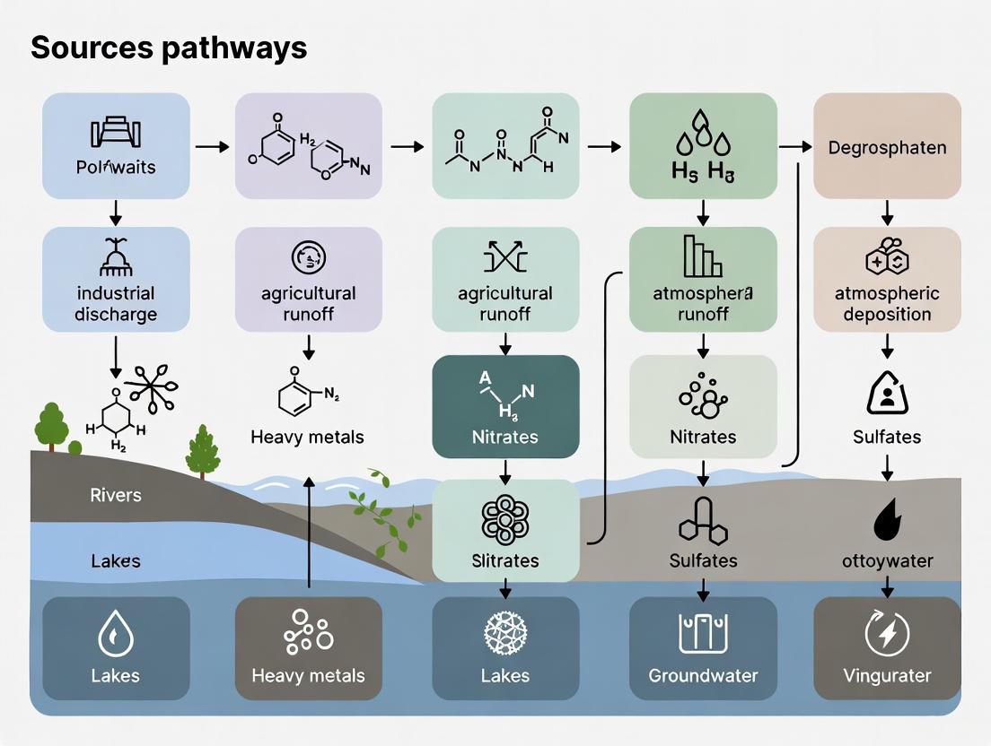
Pathways of Inorganic Pollutants in Aquatic Systems
The transport of inorganic pollutants from geogenic and anthropogenic sources to water bodies involves distinct yet sometimes interconnected pathways. Understanding these routes is crucial for intercepting contaminant fluxes.
Geogenic Pathways are primarily governed by hydrological and weathering processes. Heavy metals naturally present in bedrock and soils are mobilized through chemical weathering and soil erosion [9] [10]. Rainfall and surface runoff then transport these mobilized contaminants into groundwater aquifers via infiltration or into rivers and lakes through surface runoff [10]. Additionally, atmospheric deposition from natural sources like volcanic activity and dust storms can contribute metals directly to water surfaces [9] [10].
Anthropogenic Pathways are more diverse and often result in higher localized concentrations. Industrial discharges from mining, smelting, and manufacturing facilities release effluents directly into water bodies (point sources) [10]. Urban wastewater systems, including untreated sewage and combined sewer overflows (CSOs), discharge nutrients, pharmaceuticals, and heavy metals [11] [10]. Agricultural runoff transports fertilizers and pesticides containing heavy metals from fields to streams, a classic non-point source [9] [10]. The interaction of stormwater and wastewater in sewer systems during extreme rainfall events leads to CSOs, which release untreated pollutants like pharmaceuticals (e.g., Carbamazepine, Ciprofloxacin) and organic compounds directly into rivers [11].
The following diagram synthesizes these primary pathways and their interactions within the aquatic environment.
The Scientist's Toolkit: Research Reagent Solutions
This section details key reagents, materials, and software solutions essential for conducting research on inorganic pollutants in water, as cited in the methodologies discussed.
Table 2: Essential Reagents and Materials for Water Pollutant Research
| Item | Function/Application | Technical Specification / Example |
|---|---|---|
| ICP-MS Calibration Standards | Quantifying heavy metal (Cu, Zn, Cd, Cr) concentrations with high sensitivity. | Certified multi-element standard solutions traceable to NIST [9]. |
| Sample Preservation Reagents | Acidifying water samples to prevent adsorption of metals to container walls. | High-purity nitric acid (HNO₃), trace metal grade, to pH < 2 [9]. |
| Filtration Membranes | Separating dissolved and particulate metal fractions for speciation analysis. | 0.45 micrometer pore size, polyethersulfone or cellulose acetate [9]. |
| GIS Software | Spatial analysis, mapping pollution hotspots, and integrating land-use data. | Platforms like ArcGIS or QGIS for spatial heterogeneity analysis [11]. |
| Statistical Modeling Software | Running Random Forest models and other multivariate analyses. | R programming language with 'randomForest' package or Python with scikit-learn [9]. |
| Hydrological Simulation Software | Modeling urban runoff and combined sewer overflow (CSO) events. | EPA's Storm Water Management Model (SWMM) platform [11]. |
The intricate challenge of inorganic water pollution demands a clear and quantitative understanding of its dual origins in geogenic deposits and industrial discharges. While geogenic sources provide a regional background concentration, anthropogenic activities are the dominant drivers of severe pollution hotspots and elevated loads in global inland waters. Climate change and urbanization are exacerbating this issue, intensifying the temporal variability and severity of pollutant discharges [11] [9]. Tackling this problem effectively requires transdisciplinary research and cross-border communication, merging sound science with adaptable legislation and management systems [10]. The methodologies and data synthesized in this whitepaper provide a scientific foundation for targeting pollution control in vulnerable regions and developing sustainable water quality management strategies for the future.
The management and preservation of global water resources are critically dependent on understanding the primary pathways through which inorganic pollutants enter aquatic ecosystems. This technical guide examines three principal conduits—agricultural runoff, industrial effluents, and corroded infrastructure—as integrated components of a larger hydrological pollution system. These pathways facilitate the transport of pervasive inorganic contaminants, including heavy metals, nutrients, and saline ions, which pose significant risks to environmental stability and public health [12] [13]. The persistence, ability to bioaccumulate, and complex interactions of these pollutants within water matrices make them particularly challenging to manage [12]. Furthermore, infrastructure corrosion is not merely a consequence of water quality but an active, self-reinforcing contributor that can exacerbate pollutant release [14]. This document synthesizes current research on the sources, characteristics, and transport mechanisms of these pollutants, providing a scientific foundation for targeted mitigation strategies and future research directions essential for protecting vital water resources.
Agricultural Runoff
Agricultural runoff represents a significant non-point source of water pollution, characterized by its diffuse origin and complex composition. The primary inorganic contaminants originate from the extensive application of fertilizers, pesticides, and soil amendments [13]. Key pollutants include:
- Nutrients: Total Nitrogen (TN) and Total Phosphorus (TP) from fertilizers, which drive eutrophication [13].
- Heavy Metals: Cadmium (Cd) and lead (Pb) are frequently present in agricultural soils, often introduced via impurities in phosphate fertilizers and certain pesticides [13] [15]. These metals can accumulate in sediments and bioaccumulate in the food chain.
- Salts and Ions: Potassium (K), calcium (Ca), magnesium (Mg), chloride (Cl⁻), and bicarbonate (HCO₃⁻) can be mobilized from soils and contribute to the freshwater salinization syndrome [16] [13].
The concentration of these substances varies significantly based on land management practices, soil type, and hydrological conditions.
Transport Pathways and Environmental Fate
The transport of agricultural pollutants to water resources is governed by overland flow and subsurface drainage. During precipitation or irrigation events, water that cannot infiltrate the soil surface flows overland, picking up and carrying dissolved contaminants and sediment-bound particles into nearby streams, rivers, and groundwater systems [13]. The "Critical Pathway" diagram below illustrates this journey from source to receptor.
Figure 1: Critical Pathway of Agricultural Runoff. This diagram visualizes the sequence from pollutant application to environmental impact, highlighting the non-point source nature of agricultural contamination.
The environmental fate of these pollutants is complex. Nutrients like nitrogen and phosphorus can stimulate excessive algal growth in receiving waters, leading to eutrophication, hypoxia, and fish kills [13]. Heavy metals tend to adsorb to sediment particles and can accumulate in riverbeds and estuaries, creating long-term contamination sinks [13] [15].
Experimental Protocol for Monitoring and Analysis
A standardized protocol for quantifying pollutant load in agricultural runoff is essential for research and regulatory compliance.
1. Watershed Delineation and Sampling Site Selection:
- Define the hydrological boundaries of the agricultural catchment area using topographic maps (e.g., USGS 7.5-minute series) or Geographic Information Systems (GIS) software [13].
- Establish sampling points at the catchment outlet and at key intermediate points representing different land uses or sub-catchments.
2. Automated Sampling and Flow Measurement:
- Install automated water samplers (e.g., ISCO 6712) programmed to collect samples based on flow-proportional or time-paced intervals, with increased frequency during and after storm events [16].
- Use flow meters (e.g., acoustic Doppler current profilers) to continuously measure discharge at the catchment outlet. This allows for the calculation of pollutant load (concentration × flow rate).
3. Field and Laboratory Analysis:
- In-Situ Measurements: Using multi-parameter sondes (e.g., YSI EXO2), measure pH, Electrical Conductivity (EC), Dissolved Oxygen (DO), and Temperature at each site.
- Laboratory Analysis:
- Nutrients: Analyze for TN and TP using standard methods such as persulfate digestion followed by colorimetric analysis on a flow injection analyzer (FIA) or discrete analyzer [13].
- Major Ions: Measure K, Ca, Mg, Cl⁻, HCO₃⁻ using Ion Chromatography (IC) [16] [13].
- Heavy Metals: Filter water samples through a 0.45 µm membrane and analyze for Cd, Pb, and other metals using Inductively Coupled Plasma Mass Spectrometry (ICP-MS) [13].
4. Data Analysis and Load Calculation:
- Pollutant load is calculated by integrating concentration and flow data over time. Statistical analysis (e.g., regression) is used to correlate land use practices with pollutant export.
Table 1: Characteristic Pollutant Profiles in Agricultural Runoff
| Pollutant Category | Specific Parameters | Typical Concentration Ranges | Primary Environmental Risk |
|---|---|---|---|
| Macro-Nutrients | Total Nitrogen (TN), Total Phosphorus (TP) | TN: 1-10 mg/L; TP: 0.1-1 mg/L [13] | Eutrophication, hypoxia, algal blooms [13] |
| Heavy Metals | Cadmium (Cd), Lead (Pb) | Low μg/L to mg/L (soil-dependent) [13] | Toxicity, bioaccumulation in food chains [13] [15] |
| Major Ions | Potassium (K), Chloride (Cl⁻) | K: 1-10 mg/L; Cl⁻: 5-50 mg/L [13] | Freshwater salinization, altered ecosystem function [16] |
Industrial Effluents
Pollutant Diversity and Point Source Characteristics
Industrial effluents are a major point source of inorganic pollution, with composition varying drastically by industry type. Unlike agricultural runoff, these discharges originate from discrete, identifiable locations such as discharge pipes [15]. The table below summarizes key industrial sectors and their characteristic inorganic pollutants.
Table 2: Industrial Sources and Associated Inorganic Pollutants
| Industry Sector | Characteristic Inorganic Pollutants | Typical Concentration Ranges |
|---|---|---|
| Metal Processing & Finishing | Heavy Metals (Cu, Zn, Ni, Cr, Cd, Pb), Cyanides, Acids | Variable, can range from high μg/L to low mg/L [15] |
| Chemical Manufacturing | PFAS, Chlorobenzene, Acids, Alkalies, Residual Solvents | PFAS: ng/L to μg/L [12] [15] |
| Textile & Dye Production | Synthetic Dyes, Heavy Metals (Cu, Cr), Salt ions | High salinity; metals in μg/L range [13] [15] |
| General Process Waste | High Biochemical Oxygen Demand (BOD: 100-3000 mgO₂/L), Chemical Oxygen Demand (COD: 10-2250 mgO₂/L), variable pH (5-12) [15] |
Contaminants of Emerging Concern (CECs) from industrial sources, such as per- and polyfluoroalkyl substances (PFAS) and certain heavy metals, are particularly problematic due to their persistence, mobility, and resistance to conventional treatment processes [12] [13].
Advanced Treatment and Removal Technologies
Treating complex industrial wastewater requires advanced technologies beyond conventional methods. The following workflow illustrates the integration of these advanced processes for comprehensive pollutant removal.
Figure 2: Advanced Treatment Workflow for Industrial Effluents. This sequential process targets different pollutant classes, from resistant organics to dissolved ions and metals.
Advanced Oxidation Processes (AOPs) utilize powerful hydroxyl radicals (•OH) to destroy persistent organic contaminants like PFAS. Techniques include UV-based systems, ozonation, and electrochemical oxidation that break complex molecules into benign end-products like CO₂ and fluoride ions [17].
Next-Generation Membrane Filtration technologies, such as reverse osmosis (RO) and nanofiltration (NF), have advanced with materials like graphene oxide and ceramic composites. These membranes feature uniform, engineered pores that reduce fouling and improve rejection rates for dissolved salts, metals, and micro-pollutants [12] [17].
Resource Recovery approaches are shifting the paradigm from mere treatment to valorization. Techniques like selective adsorption and chemical precipitation are used to recover valuable metals (e.g., cobalt, nickel, copper) from mining and electronic waste effluents, creating potential revenue streams while mitigating pollution [17].
The Scientist's Toolkit: Key Research Reagents and Materials
Research on treating industrial effluents relies on a specific suite of reagents and materials.
Table 3: Essential Research Reagents for Industrial Wastewater Analysis
| Reagent / Material | Technical Function | Application Example |
|---|---|---|
| Hydroxyl Radical (•OH) Probes (e.g., Nitrobenzene) | Chemical probe to quantify the formation rate and exposure of •OH in AOPs. | Calibrating UV/H₂O₂ or ozone reactors for PFAS degradation [17]. |
| Graphene Oxide (GO) Nanoparticles | High-surface-area adsorbent and membrane coating material. | Synthesizing novel composite membranes for enhanced heavy metal rejection [17]. |
| Magnesium-Based "Green" Reagents | Precipitating agent for metals and neutralizing agent for acidity. | Neutralizing acid mine drainage and co-precipitating dissolved metals for recovery [17]. |
| Ion-Selective Electrodes & Membranes | Potentiometric sensors for specific ions (e.g., Cl⁻, F⁻, NH₄⁺). | Real-time monitoring of specific contaminant ions in treatment process streams [16]. |
Corroded Infrastructure
Corrosion as a Source and Consequence of Pollution
Corroded water and wastewater infrastructure is a critical, often overlooked, pathway for inorganic pollutants. Corrosion itself can be both a primary source of metals (e.g., from lead pipes or iron fittings) and a secondary consequence of water chemistry, creating a damaging feedback loop [14]. The global cost of corrosion is estimated at US $2.5 trillion, accounting for roughly 3.5% of global GDP, with water systems representing a significant portion [14].
Key corrosion mechanisms in water systems include:
- Uniform Corrosion: General wastage of pipe material (e.g., iron, copper) leading to the release of metal ions into the water [14].
- Pitting Corrosion: Localized attack that can perforate pipes, releasing high concentrations of metals and providing niches for bacterial growth [14].
- Microbiologically Influenced Corrosion (MIC): Biofilms formed by bacteria, such as Desulfovibrio, produce corrosive metabolites (e.g., hydrogen sulfide) that accelerate metal decay [14].
The Role of Saltwater Intrusion
A growing threat to infrastructure integrity is saltwater intrusion in tidal rivers and coastal aquifers, driven by sea-level rise, drought, and over-extraction [16]. Elevated chloride (Cl⁻) concentrations from seawater are highly corrosive and degrade pipes, storage tanks, and treatment plant components. This compromises infrastructure and simultaneously introduces saline contaminants into freshwater supplies [16]. Nearly $100 million in agricultural activity in the Mid-Atlantic alone is at risk from this phenomenon, alongside immense costs to drinking water infrastructure [16].
Experimental Protocol for Corrosion Assessment
A comprehensive methodology for assessing corrosion in water distribution and wastewater collection systems is outlined below.
1. Specimen Preparation and Exposure:
- Prepare coupons (e.g., 2.5 cm x 5.0 cm) from materials of interest (e.g., carbon steel, ductile iron, copper).
- Polish coupons to a standard surface finish, degrease, and weigh to the nearest 0.1 mg.
- Mount coupons in pipe-flow test loops or secure them within racks placed in actual pipelines or treatment tanks for in-situ exposure over a defined period (e.g., 90-180 days) [14].
2. Corrosion Rate Monitoring:
- Electrochemical Techniques: Use a Potentiostat/Galvanostat to perform Linear Polarization Resistance (LPR) and Electrochemical Impedance Spectroscopy (EIS) on electrodes made of the material under study. This provides real-time corrosion rate data.
- Weight Loss Measurement: After exposure, retrieve coupons and chemically clean them to remove corrosion products according to ASTM standard G1-03. Re-weigh the coupons to determine mass loss. The corrosion rate (CR) in millimeters per year (mm/y) is calculated as: CR = (K × W) / (A × T × D), where K is a constant, W is mass loss (g), A is area (cm²), T is time (hours), and D is density (g/cm³) [14].
3. Corrosion Product and Water Chemistry Analysis:
- Surface Analysis: Analyze the morphology and composition of corrosion products on the coupon surface using Scanning Electron Microscopy with Energy-Dispersive X-ray Spectroscopy (SEM/EDS) and X-Ray Diffraction (XRD) [14].
- Water Quality Correlations: Correlate corrosion rates with water quality parameters measured throughout the exposure period, including pH, dissolved oxygen, chloride (Cl⁻), sulfate (SO₄²⁻), and dissolved organic matter (DOM) [14].
Addressing the critical pathways of agricultural runoff, industrial effluents, and corroded infrastructure requires an integrated, multi-faceted strategy. The following approaches are essential:
- Policy and Regulation: Strengthening regulatory frameworks to include emerging contaminants and enforce stricter discharge permits, while incentivizing the adoption of best management practices in agriculture and industry [12] [13].
- Advanced and Nature-Based Solutions: Promoting the implementation of advanced treatment technologies like AOPs and precision membranes for industrial point sources, alongside the wider use of cost-effective Nature-Based Solutions (NBS) like Constructed Wetlands (CWs) for non-point source treatment, which can achieve up to 88% removal efficiency for many contaminants [13].
- Infrastructure Modernization and Monitoring: Investing in corrosion-resistant materials and smart water systems that leverage Artificial Intelligence (AI) for real-time monitoring and predictive maintenance of infrastructure [17] [14]. Enhanced monitoring of major salt ions is crucial for protecting infrastructure in vulnerable coastal areas [16].
In conclusion, the pathways of agricultural runoff, industrial effluents, and corroded infrastructure are interconnected components of the water pollution cycle. A holistic understanding of their distinct yet overlapping characteristics is the foundation for developing effective, sustainable management policies and technologies. Future efforts must focus on closing resource loops, enhancing system resilience, and fostering interdisciplinary collaboration to safeguard water resources for future generations.
This whitepaper provides an in-depth technical analysis of the health impacts of key inorganic pollutants, with a specific focus on their sources and pathways in water resources. For researchers and scientists in drug development and environmental health, understanding the mechanisms by which these pollutants exert carcinogenic, organ-damaging, and neurotoxic effects is critical for developing targeted interventions and therapeutic strategies. The complex interactions between pollutant exposure and disease pathogenesis involve multiple molecular pathways, including oxidative stress, inflammation, and DNA damage, which will be explored in detail throughout this document. Framed within the broader context of inorganic pollutant pathways in aquatic systems, this review synthesizes current findings on several priority substances, including arsenic, heavy metals, and disinfection byproducts, highlighting their toxicological profiles and the experimental approaches used to characterize them.
Carcinogenicity of Pollutants
Key Mechanisms and Associated Pollutants
The carcinogenicity of environmental pollutants is mediated through diverse mechanisms, including direct DNA damage, cancer stem cell (CSC) induction, and receptor-mediated pathways. Table 1 summarizes the carcinogenic targets and primary mechanisms of several key inorganic pollutants.
Table 1: Carcinogenic Targets and Mechanisms of Key Pollutants
| Pollutant | Target Organs (Species) | Primary Carcinogenic Mechanisms | Experimental Evidence |
|---|---|---|---|
| Inorganic Arsenic | Lung, Liver, Gallbladder, Ovary, Uterus (Mouse) [18] | Overproduction of Cancer Stem Cells (CSCs); Overexpression of COX-2 and ER-α in reproductive tissues [18] | "Whole-life" exposure model in CD1 mice (0-24 ppm in drinking water); Immunohistochemistry for CSC markers (ALDH1, CD133) [18] |
| Polycyclic Aromatic Hydrocarbons (PAHs) | Multiple (Human/Animal) [19] | Mutagenic and carcinogenic properties via metabolic activation to DNA-binding intermediates [19] | Listed as priority pollutants by EU and US EPA; Epidemiological and toxicological studies [19] |
| Heavy Metals (e.g., Cd, Cr, Ni) | Multiple (Human/Animal) [20] | Direct and indirect DNA damage; Inhibition of DNA repair; Oxidative stress via Fenton reaction (Cr, Ni, Co) [20] | In vitro and in vivo studies showing DNA base modification, crosslinking, and strand scission [20] |
Detailed Experimental Protocol: "Whole-Life" Arsenic Carcinogenesis Bioassay
The following methodology details a comprehensive in vivo approach for assessing the carcinogenic potential of inorganic arsenic, replicating chronic human exposure scenarios [18].
- Animal Model and Husbandry: The study employs CD1 mice. The animal facility should be accredited (e.g., by AAALAC), with controlled temperature, humidity, and light cycles. Animals are provided with a basal diet and acidified water ad libitum [18].
- Test Article and Dosing: Sodium arsenite (NaAsO₂, ≥98% purity) is dissolved in drinking water at concentrations of 0 (control), 6, 12, and 24 ppm arsenic. These doses capture the upper range of human environmental exposure [18].
- Experimental Design and "Whole-Life" Exposure Protocol:
- Pre-breeding: Male and female breeder mice are exposed to arsenic-treated water two weeks prior to mating.
- Gestation and Lactation: Pregnant dams continue exposure throughout pregnancy and lactation.
- Offspring Exposure: At weaning (4 weeks of age), offspring are randomly selected (n=30/sex/dose) and continue to receive the same arsenic-treated water until the study termination at 104 weeks [18].
- Tissue Collection and Histopathological Analysis:
- A complete necropsy is performed on all moribund animals, animals found dead, and at terminal sacrifice.
- A comprehensive set of tissues (e.g., liver, lungs, kidneys, adrenals, reproductive organs, and all gross lesions) is collected.
- Tissues are fixed in 10% neutral buffered formalin, embedded in paraffin, sectioned at 5 μm, and stained with Hematoxylin and Eosin (H&E) for blinded pathological assessment [18].
- Immunohistochemical Analysis:
- Paraffin-embedded sections of tumors and target tissues are used.
- Key biomarkers include:
- CSC Markers: ALDH1 and CD133 to identify and quantify cancer stem cell populations.
- Receptor and Signaling Markers: Estrogen receptor-α (ER-α), cyclin D1, cyclooxygenase-2 (Cox-2), and NF-κB to investigate proliferative and inflammatory pathways [18].
Diagram 1: Arsenic Carcinogenicity Assessment Workflow
Pollutant-Induced Organ Damage
Liver Damage and NAFLD
Environmental contaminants in water resources are increasingly implicated in the development and progression of nonalcoholic fatty liver disease (NAFLD). The global prevalence of NAFLD is over 25%, and environmental risk factors are now a key area of investigation [21]. Several pollutants have been identified as contributors to liver pathology through mechanisms involving lipid metabolism disruption and oxidative stress. Table 2 outlines the specific mechanisms by which different pollutant classes drive NAFLD.
Table 2: Mechanisms of Pollutant-Induced Liver Damage and NAFLD
| Pollutant Class | Specific Examples | Key Mechanisms in NAFLD/Liver Damage | Research Evidence |
|---|---|---|---|
| Heavy Metals | Arsenic, Cadmium, Lead [21] [20] | Oxidative stress; depletion of glutathione; inhibition of antioxidant enzymes; disruption of lipid metabolism pathways [20]. | Toxicological studies showing bioaccumulation in liver tissue; epidemiological associations [21] [20]. |
| Disinfection By-products (DBPs) | Trihalomethanes, Haloacetic acids [21] | Oxidative stress and lipid peroxidation; metabolic disruption leading to steatosis [21]. | Positive associations in epidemiological studies; supported by toxicological data in animal models [21]. |
| Persistent Organic Pollutants (POPs) | Dioxins, Polychlorinated Biphenyls (PCBs) [21] | Activation of aryl hydrocarbon receptor (AhR); induction of cytochrome P450 enzymes; disruption of energy homeostasis [21]. | Analysis of great many epidemiological and toxicological studies [21]. |
| Microcystins (MCs) | MC-LR [21] | Potent inhibition of protein phosphatases 1 and 2A; leading to oxidative stress and cytoskeletal disruption [21]. | Strong evidence from toxicological studies [21]. |
Gut Microbiome Dysbiosis and Systemic Inflammation
The gut microbiome serves as a critical interface for ingested inorganic pollutants, playing a dual role in modulating their toxicity and being disrupted by them. This interaction represents a significant pathway for systemic organ damage [22].
- Heavy Metals (Arsenic, Cadmium, Lead): Exposure can directly alter bacterial community structure, reducing beneficial commensals and selecting for more harmful pathogens. This dysbiosis drives inflammation through metabolite production and activation of signaling pathways such as the LPS/TLR4 or proteoglycan/TLR2 pathways, contributing to a leaky gut and systemic inflammation [22].
- Persistent Organic Pollutants (POPs): Pollutants like PCB-126 can activate the aryl hydrocarbon receptor (AHR) within the intestine. This activation can, in turn, indirectly reshape the gut microbial composition, creating a pro-inflammatory milieu [22].
- Nitrates/Nitrites: The effect of these compounds on the host is heavily dependent on their transformation by gut bacteria into secondary and tertiary metabolites, including nitrosamines, which can have systemic toxic and carcinogenic effects [22].
Diagram 2: Gut-Liver Axis in Pollutant Toxicity
Neurotoxicity of Pollutants
Mechanisms and Neurological Outcomes
The nervous system is highly vulnerable to chemical insult, with over 850 chemicals known to produce neurobehavioral disorders [23]. Neurotoxicity can manifest as cognitive deficits, neurodevelopmental abnormalities, and neurodegenerative diseases. The developing nervous system is often uniquely susceptible to damage that can lead to permanent functional impairment [23]. Table 3 details the neurotoxic mechanisms of specific pollutant classes, with a focus on chlorinated disinfection byproducts (Cl-DBPs) and heavy metals.
Table 3: Neurotoxic Pollutants: Mechanisms and Functional Outcomes
| Pollutant Class/Example | Molecular/Cellular Mechanisms | Neurological Manifestations & Outcomes | Experimental Support |
|---|---|---|---|
| Cl-DBPs (e.g., DCA, TCA, DCBQ) | Induction of oxidative stress & ER stress; DNA damage; inflammation (NF-κB); apoptosis & autophagy [24]. | Peripheral neuropathy; anxiety-like behavior; thermal hypoalgesia; reduced nerve conduction velocity; potential risk for neurodevelopmental & neurodegenerative diseases [24]. | In vitro studies on nerve cells; animal models showing behavioral and functional deficits [24]. |
| Heavy Metals (e.g., Lead, Mercury) | Binding to sulfhydryl groups of proteins; generation of ROS; mitochondrial dysfunction [23] [20]. | Cognitive deficits; irreversible compromise of normal brain development in children; peripheral neuropathies [23]. | Extensive epidemiological data (e.g., lead); clinical experience; NIOSH identification as a leading work-related disorder [23]. |
| Organic Pesticides (e.g., Oxyfluorfen) | Inhibition of acetylcholinesterase (AChE) activity; oxidative stress [25]. | Neurotoxic effects in non-target species; significant AChE inhibition reported in bivalves [25]. | Eco-toxicological bioassays using biomarkers in model organisms like C. edule [25]. |
Detailed Experimental Protocol: Assessing Neurotoxicity in Marine Bivalves
This protocol utilizes the marine bivalve Cerastoderma edule as a bioindicator species to evaluate the neurotoxic effects of pollutants, incorporating the impact of abiotic factors like temperature [25].
- Organism Collection and Acclimation:
- Organisms (e.g., C. edule) are collected from a defined field site and transported to the laboratory in cold boxes with field water.
- In the laboratory, they are acclimated in glass aquariums with filtered seawater (salinity 20 PSU) for 48 hours with constant aeration. During acclimation, organisms are not fed. After acclimation, they are fed daily with a commercial microalgae mixture [25].
- Chemical Exposure and Bioassay:
- Test Chemicals: Stock solutions are prepared. For organic chemicals like oxyfluorfen, a solvent (e.g., acetone) may be used, ensuring the final concentration is below OECD guideline limits (e.g., <0.01%). For inorganic metals like copper, the stock is prepared directly in filtered seawater [25].
- Experimental Design: Organisms are exposed to a range of chemical concentrations (e.g., Cu from 81.25 to 605.58 µg L⁻¹; Oxyfluorfen from 1.88 to 21.36 mg L⁻¹) at different temperatures (e.g., 15°C, 20°C, 25°C) for 96 hours. Controls (negative and solvent control) are included [25].
- Vessel Material: Following OECD guidelines, plastic vessels are used for inorganic chemicals (e.g., Cu), and glass vessels for organic chemicals (e.g., Oxyfluorfen) [25].
- Biomarker Analysis as a Proxy for Neurotoxicity:
- Post-exposure, organisms are dissected, and tissues are homogenized for biochemical analysis.
- Primary Neurotoxicity Biomarker: Acetylcholinesterase (AChE) activity is a key diagnostic biomarker. Significant inhibition of AChE indicates neurotoxic effects [25].
- Supplementary Biomarkers:
- Antioxidant Defense Enzymes: Catalase (CAT), Glutathione S-transferase (GST), Glutathione Reductase (GR), Glutathione Peroxidase (GPx) to assess oxidative stress response.
- Oxidative Damage: Thiobarbituric Reactive Substances (TBARS) levels are measured to indicate lipid peroxidation (LPO) [25].
- Data and Statistical Analysis: Dose-response and temperature-dependent effects are analyzed to determine LC50 values and sub-lethal biomarker responses.
Diagram 3: Neurotoxicity Pathways of Pollutants
The Scientist's Toolkit: Research Reagent Solutions
This section details essential reagents, models, and methodologies used in the featured studies for investigating pollutant impacts.
Table 4: Key Research Reagents and Models for Pollutant Impact Studies
| Tool/Category | Specific Example | Function/Application | Reference |
|---|---|---|---|
| In Vivo Model | CD1 Mouse | A robust, outbred strain for chronic carcinogenicity bioassays and "whole-life" exposure studies. | [18] |
| In Vivo/ Bioindicator Model | Cerastoderma edule (Marine Bivalve) | A bioindicator species for ecotoxicological studies; used to assess lethal and sub-lethal toxicity (e.g., neurotoxicity) under varying environmental conditions. | [25] |
| Test Chemical | Sodium Arsenite (NaAsO₂) | A common, well-characterized source of inorganic arsenic (AsIII) for preparing dosing solutions in toxicological studies. | [18] |
| Histology Stain | Hematoxylin and Eosin (H&E) | The standard staining protocol for histological analysis of tissue morphology and identification of pathological lesions, including tumors. | [18] |
| Immunohistochemistry Antibodies | Anti-ALDH1, Anti-CD133, Anti-ER-α, Anti-COX-2 | Used to detect and localize specific proteins in tissue sections (e.g., cancer stem cell markers, hormone receptors, inflammatory enzymes). | [18] |
| Biomarker Assays | Acetylcholinesterase (AChE) Activity | A key enzymatic biomarker for diagnosing neurotoxic effects, particularly for organophosphates and other contaminants. | [25] |
| Biomarker Assays | Catalase (CAT), GST, GPx, GR Activity | A suite of enzymatic assays to profile the antioxidant defense system and oxidative stress status in exposed organisms. | [25] |
| Oxidative Damage Assay | Thiobarbituric Reactive Substances (TBARS) | A common method to quantify lipid peroxidation, a key indicator of oxidative damage to cell membranes. | [25] |
| Analytical Tool | Mass Spectrometry | Advanced chemical analysis for detecting thousands of markers in biological samples (blood, urine) in exposomic studies. | [26] |
| Computational Framework | Exposomics | A data-driven approach to map all environmental exposures throughout life, using geospatial data, wearables, and AI. | [26] |
Arsenic, a naturally occurring metalloid, represents a significant global health concern due to its pervasive presence in the environment and potent toxicity. This case study examines the pathways through which arsenic moves from geological deposits into water resources, its systemic toxic effects on the human body, and its well-established role in carcinogenesis. Framed within the broader context of inorganic pollutants in water resources research, this analysis synthesizes current understanding of arsenic contamination dynamics, with particular attention to the interplay between natural biogeochemical processes and human activities that mobilize this toxic element. The World Health Organization estimates that over 200 million people worldwide are exposed to toxic levels of arsenic through contaminated drinking water, making arsenic a priority substance for environmental health research and regulatory action [27].
Arsenic occurs naturally in the Earth's crust and enters the environment through both natural processes and anthropogenic activities. Natural sources include volcanic activity, rock weathering, and mineral dissolution, while human activities such as mining, smelting, agricultural pesticide use, and industrial processes contribute to arsenic mobilization [28] [27]. The distribution of arsenic in groundwater exhibits significant geographical variation, with some of the highest concentrations reported in Bangladesh, India, Taiwan, and Chile [28] [27]. A recent study in Bangladesh's Gazipur industrial zone revealed that while arsenic concentrations (0.003 ± 0.004 mg/L) remained within acceptable limits, lead, iron, and manganese exceeded safe drinking water standards, illustrating the complex coexistence of multiple metallic contaminants in affected aquifers [29].
Hydrobiogeochemical Cycling
The mobility of arsenic in aquatic systems is governed by complex biogeochemical processes. A 2025 study revealed a previously underestimated pathway for arsenic pollution involving the shift of lake and river sediments from arsenic sinks to arsenic sources following the widespread loss of submerged aquatic plants [30]. These underwater macrophytes, such as Vallisneria natans, play a crucial protective role by releasing oxygen through their roots, creating conditions that promote the formation of iron plaques that trap and immobilize arsenic in sediments [30].
When these plants die due to water pollution or climate change, the system undergoes a dramatic transition from aerobic to anaerobic conditions. This shift dissolves the iron plaques and releases arsenic back into the water column. Research documented that after plant death, the abundance of iron-reducing bacteria surged by over 80%, contributing to a nearly 90% loss of arsenic once bound within the roots' protective iron plaque [30]. This pathway represents a significant feedback loop wherein environmental degradation begets further water quality deterioration.
Table 1: Key Hydrobiogeochemical Processes Affecting Arsenic Mobility
| Process | Conditions | Effect on Arsenic | Environmental Significance |
|---|---|---|---|
| Reductive Dissolution | Anaerobic, high organic matter | Releases bound arsenic | Major mobilization mechanism in groundwater [29] |
| Oxidative Immobilization | Aerobic, presence of iron | Traps arsenic in iron plaques | Protective mechanism in vegetated sediments [30] |
| Plant-Mediated Rhizosphere Oxidation | Aerated root zones | Immobilizes arsenic | Submerged macrophytes as ecosystem protectors [30] |
| Microbial Iron Reduction | Anaerobic, bacterial activity | Releases arsenic | Contributes to arsenic mobilization after plant death [30] |
Systemic Toxicity and Pathophysiological Mechanisms
Arsenic Speciation and Toxicokinetics
The toxicity of arsenic depends critically on its chemical form and oxidation state. Arsenic exists in four common valence states: elemental arsenic (As0), arsenite (trivalent, AsIII), arsenate (pentavalent, AsV), and arsine gas [28]. In general, inorganic forms are more toxic than organic forms, and trivalent arsenic compounds are more toxic than pentavalent compounds [31]. The metabolism of arsenic involves reduction from pentavalent to trivalent state followed by oxidative methylation, with the trivalent methylated metabolites now recognized as highly toxic species [32].
Approximately 60-90% of ingested inorganic arsenic is absorbed through the gastrointestinal tract, with initial distribution to the liver, kidney, muscle, and skin [28]. Excretion occurs primarily through the renal system, with only about 30% of inorganic arsenic eliminated within the first week, contributing to its cumulative toxicity [28].
Molecular Mechanisms of Toxicity
Arsenic induces cellular injury and death through multiple interconnected mechanisms:
Interference with Cellular Respiration and Energy Production At a biochemical level, trivalent arsenic (arsenite) reacts with sulfhydryl groups of critical enzymes, including those in the pyruvate oxidation pathway and the tricarboxylic acid cycle [31]. This inhibition disrupts cellular respiration and impairs ATP production. Pentavalent arsenic (arsenate) can replace phosphate in biochemical reactions due to their similar structure and properties, leading to the formation of unstable compounds such as glucose-6-arsenate that disrupt glycolysis [32]. The replacement of stable phosphorus with arsenic in ATP formation results in rapid hydrolysis of high-energy bonds, effectively uncoupling mitochondrial respiration [31].
Oxidative Stress Arsenic metabolism generates reactive oxygen species, increasing oxidative stress and damaging DNA, lipids, and other macromolecules [27]. This oxidative damage contributes to both the toxic and carcinogenic effects of arsenic.
Protein Dysregulation Arsenite's affinity for thiol groups allows it to bind and inhibit numerous proteins and enzymes. It specifically binds to thiol group-containing hormone receptors, potentially explaining its diabetogenic effect through inhibition of insulin receptor function [31].
Table 2: Arsenic Species and Their Toxicological Properties
| Arsenic Species | Common Forms | Relative Toxicity | Major Mechanisms | Primary Sources |
|---|---|---|---|---|
| Inorganic Trivalent | Arsenite (AsIII) | Highest | Binds to protein thiol groups; inhibits cellular respiration [31] | Groundwater, industrial processes |
| Inorganic Pentavalent | Arsenate (AsV) | High | Replaces phosphate in biochemical reactions [32] | Groundwater, industrial processes |
| Organic Trivalent | MMAIII, DMAIII | High to Moderate | Binds to protein thiol groups; genotoxic [32] | Biological metabolites |
| Organic Pentavalent | MMAV, DMAV | Lower | Limited reactivity; some oxidative stress [31] | Seafood, biological metabolites |
| Elemental Arsenic | As0 | Low | Poor solubility [31] | Environmental dust |
| Arsine Gas | AsH3 | Extreme | Hemolytic agent [28] [31] | Industrial accidents |
Clinical Manifestations of Toxicity
The clinical presentation of arsenic poisoning varies based on exposure duration and intensity:
Acute Toxicity Acute exposure typically presents with gastroenteritis (nausea, vomiting, diarrhea, abdominal pain) within minutes to hours, followed by hypotension and cardiovascular effects including EKG abnormalities such as QTc prolongation [28]. High-dose exposures can lead to multi-organ failure and death [32].
Chronic Toxicity Chronic exposure affects multiple organ systems, with characteristic dermatological manifestations including hyperpigmentation with "raindrop" appearance, hyperkeratosis of palms and soles, and Mees' lines (transverse white bands on nails) [28]. Neurological effects include sensorimotor polyneuropathy presenting as dysesthesias in a stocking-glove distribution [28]. Other effects include cardiovascular disease, diabetes, and various cancers [28] [32].
Carcinogenic Mechanisms and Evidence
Epidemiological Evidence
The International Agency for Research on Cancer (IARC) classifies arsenic as a Group I human carcinogen, with strong evidence linking exposure to cancers of the skin, lung, bladder, and kidney [27]. Epidemiological studies have demonstrated increased cancer incidence in populations with elevated arsenic exposure from drinking water, with evidence from Chilean cohorts showing increased lung cancer incidence during high-exposure periods [27]. Similarly, mitigation efforts in Taiwan that reduced arsenic in drinking water subsequently decreased lung cancer rates [27].
Mechanisms of Carcinogenesis
Arsenic carcinogenesis involves multiple complex mechanisms that remain incompletely understood. Current evidence suggests contributions from several interconnected pathways:
Genotoxicity and Oxidative Stress Arsenic generates reactive oxygen species that cause DNA damage, including strand breaks and oxidative lesions [27]. Concurrently, arsenic inhibits DNA repair mechanisms, creating a permissive environment for mutations to accumulate [27].
Altered Epigenetic Regulation Arsenic modifies DNA methylation patterns and other epigenetic markers, potentially altering gene expression in ways that promote carcinogenesis [27]. Studies have shown altered methylation of the p53 tumor suppressor promoter in lung cells exposed to arsenic [32].
Altered Cell Signaling and Proliferation A 2025 network-based analysis constructed an adverse outcome pathway framework for arsenic-induced lung cancer, identifying activation of the EGFR and PI3K/AKT pathways as key events leading to dysregulated cell proliferation and lung carcinogenesis [33]. Arsenic can also replace zinc in zinc finger proteins, potentially disrupting transcription factor function and cellular signaling [27].
Cocarcinogenesis and Tumor Promotion Arsenic may act as a cocarcinogen by enhancing the effects of other carcinogens and promoting the growth of initiated cells through altered growth factor expression and chronic cellular proliferation [32].
Analytical Methodologies and Experimental Approaches
Arsenic Speciation Analysis
The determination of individual arsenic species is critical for accurate toxicity assessment, as different species exhibit markedly different toxicities. Hyphenated techniques combining high-efficiency separation with highly sensitive detection have become the methods of choice [34]. These include:
- High-performance liquid chromatography with inductively coupled plasma mass spectrometry (HPLC-ICP-MS) for sensitive element-specific detection
- Hydride generation atomic spectrometry for specific arsenic forms
- Electrospray mass spectrometry for molecular identification
Reliable speciation analysis requires careful methods for extracting arsenic species from solid samples while preserving species integrity, and stabilizing species in solutions to prevent interconversion [34].
Microscale Sampling and Molecular Analysis
Advanced techniques for monitoring arsenic transformation in environmental and biological systems include:
Microscale Sampling of Sediment Profiles High-resolution sampling of sediment layers at millimeter scale near plant root zones allows detailed mapping of arsenic, iron, and microbial activity gradients [30]. This approach reveals the sharp transitions between oxidized and reduced zones that control arsenic mobility.
High-Throughput Genetic Sequencing Comprehensive analysis of microbial community structure and functional genes through 16S rRNA sequencing and metagenomics identifies arsenic-responsive taxa and metabolic pathways [30]. This technique documented an over 80% increase in iron-reducing bacteria following plant death and the subsequent release of arsenic.
Gene Expression Analysis Quantitative assessment of bacterial genes involved in arsenic transformation, including arsenate reductase genes and those responsible for converting toxic arsenic forms to less toxic ones, provides mechanistic insights into arsenic cycling [30].
Diagram 1: Arsenic Metabolism and Carcinogenesis Pathways. This diagram illustrates the metabolic activation of arsenic through sequential reduction and methylation steps, and the multiple interconnected pathways contributing to arsenic carcinogenesis, including oxidative stress, DNA damage, epigenetic alterations, and dysregulated cell proliferation.
The Scientist's Toolkit: Research Reagent Solutions
Table 3: Essential Research Reagents for Arsenic Toxicology Studies
| Research Reagent | Function and Application | Experimental Context |
|---|---|---|
| Inductively Coupled Plasma Mass Spectrometry (ICP-MS) | Ultra-trace quantification of arsenic and other metals in environmental and biological samples [29] | Detection of arsenic in water samples from contaminated areas [29] |
| High-Performance Liquid Chromatography (HPLC) Systems | Separation of arsenic species prior to detection [34] | Arsenic speciation analysis for toxicity assessment [34] |
| High-Throughput Genetic Sequencers | Comprehensive analysis of microbial community structure and functional genes [30] | Identification of arsenic-responsive taxa and metabolic pathways in sediments [30] |
| Microscale Sampling Probes | High-resolution sampling of sediment and water profiles at millimeter scale [30] | Mapping arsenic, iron, and microbial activity gradients in sediment profiles [30] |
| Cell Culture Models (e.g., HBE cells) | In vitro systems for studying arsenic toxicity and transformation mechanisms [33] | Investigation of arsenic-induced malignant transformation in human bronchial epithelial cells [33] |
| Atomic Absorption Spectrometry with Hydride Generation | Sensitive detection of specific arsenic forms [34] | Quantification of inorganic arsenic species in environmental samples [34] |
Diagram 2: Aquatic Plant Mediated Arsenic Cycling. This workflow illustrates the dual role of submerged aquatic vegetation in arsenic dynamics, showing how healthy plants immobilize arsenic through root oxygen release and iron plaque formation, while plant death triggers a cascade of events leading to arsenic mobilization through microbial activity and changing redox conditions.
This case study demonstrates the complex journey of arsenic from natural geological deposits to a systemic toxicant and human carcinogen, with water resources serving as the critical exposure pathway for human populations. The mechanisms underlying arsenic toxicity and carcinogenesis involve multiple interconnected pathways, including metabolic activation, interference with cellular energy production, oxidative stress, genotoxicity, and altered gene expression. Recent research has revealed previously underestimated environmental pathways, particularly the role of aquatic ecosystem health in determining whether sediments function as arsenic sinks or sources. Future research directions should focus on elucidating the dose-response relationships at low exposure levels, clarifying the relative contributions of different carcinogenic mechanisms, and developing integrated strategies for preventing arsenic mobilization in aquatic systems. Protecting and restoring submerged aquatic vegetation emerges as a critical component of comprehensive arsenic risk management in water resources, highlighting the intricate connections between ecosystem health and human toxicological outcomes.
Within the broader study of inorganic pollutant sources and pathways in water resources, nitrate (NO₃⁻) and nitrite (NO₂⁻) represent a pervasive class of contaminants with direct and acute human health implications. These nitrogen-oxygen ions are a natural part of the nitrogen cycle but have become concentrated in water systems globally due to intensive agricultural practices, industrial activities, and sewage discharge [35] [36] [37]. The most well-established and dangerous acute health effect from elevated nitrate/nitrite exposure is methemoglobinemia, a condition that impairs blood oxygen transport. This case study provides an in-depth technical examination of the mechanistic pathway of methemoglobinemia, supported by quantitative exposure data, experimental insights into clinical diagnosis, and an overview of relevant research methodologies.
Nitrate and nitrite enter water resources through multiple pathways, with agricultural activity being the dominant source. The overapplication of nitrogen-based fertilizers and animal manure leads to nitrate leaching into groundwater, particularly in shallow, rural domestic wells [35] [38]. Other significant sources include septic systems, wastewater discharge, and industrial waste [36] [15].
Table 1: Primary Sources of Nitrate and Nitrite in Water Resources
| Source Category | Specific Examples | Key Characteristics & Pathways |
|---|---|---|
| Agricultural | Nitrogen-based fertilizers (e.g., potassium nitrate, ammonium nitrate), animal manure [35] [38] | Nitrates are highly water-soluble and readily migrate into groundwater; most prevalent in agricultural areas [35]. |
| Wastewater | Septic systems, sewage discharge, landfill leachate [35] [36] [15] | A major problem in areas with high population density, small lot sizes, or inadequate treatment infrastructure [38]. |
| Industrial | Manufacturing processes, boiler fluid additives, food processing (preservatives) [35] [15] | Can involve direct discharge of nitrites or organic nitrogen wastes that are broken down [35]. |
Human exposure occurs predominantly through the consumption of contaminated drinking water and food. For bottle-fed infants, the primary exposure source is contaminated drinking water used to prepare formula [35] [39]. The scale of the problem is significant; a global assessment revealed that during 1970–2010, populations potentially affected by chronic health risks from surface-water nitrate exposure increased from 169 to 1361 million persons per year [37].
Table 2: Typical Nitrate Content in Selected Vegetables (Fresh Weight)
| Vegetable | Nitrate Content (mg/100g) [35] |
|---|---|
| Spinach, Lettuce, Red Beetroot, Celery | Very High (> 2500) |
| Parsley, Leek, Chinese Cabbage | High (1000–2500) |
| Cabbage, Dill, Turnip | Medium (500–1000) |
| Broccoli, Carrot, Cauliflower | Low (200–500) |
| Asparagus, Tomato, Onion, Green Bean | Very Low (< 200) |
The Mechanism of Methemoglobinemia
Methemoglobinemia, commonly known as "blue baby syndrome," is an acute health condition that impairs the blood's oxygen-carrying capacity. The following diagram illustrates the key biochemical pathway and physiological consequences.
Figure 1: Biochemical pathway of nitrate-induced methemoglobinemia.
The mechanism involves a multi-step process triggered after nitrate is ingested and converted to nitrite [39] [37]:
- Ingestion and Conversion: Nitrate (NO₃⁻) is consumed via contaminated water or food. In the gastrointestinal tract, particularly under less acidic conditions or in the presence of certain bacteria, nitrate is reduced to nitrite (NO₂⁻) [37].
- Absorption and Oxidation: Nitrite is absorbed into the bloodstream where it reacts with hemoglobin in red blood cells. Nitrite oxidizes the iron atom in the heme group of hemoglobin from its ferrous state (Fe²⁺) to the ferric state (Fe³⁺), converting hemoglobin to methemoglobin [37].
- Physiological Consequence: Methemoglobin cannot bind oxygen, leading to a reduced oxygen-carrying capacity of the blood. This results in tissue hypoxia, the underlying cause of clinical symptoms such as cyanosis (a bluish discoloration of the skin), headache, fatigue, tachycardia, and in severe cases, asphyxia and death [37].
Infants under six months are particularly susceptible due to several factors: larger fluid intake relative to body weight, lower stomach acidity (favoring bacterial reduction of nitrate to nitrite), higher levels of fetal hemoglobin (which is more easily oxidized), and lower activity of the enzyme NADH-cytochrome b5 reductase, which is responsible for reducing methemoglobin back to functional hemoglobin [39] [37].
Quantitative Health Risks and Regulatory Standards
The health risk is directly correlated with the concentration of nitrate/nitrite in drinking water. Regulatory standards are established to prevent methemoglobinemia, though emerging research suggests chronic risks may occur at levels below these standards [37].
Table 3: Health Risk Thresholds and Regulatory Standards for Nitrate/Nitrite in Drinking Water
| Concentration (as Nitrate-Nitrogen, ppm) | Health Risk & Regulatory Status |
|---|---|
| > 3 ppm | Cautionary Level: Suggests potential contamination. Recommendation is to test water periodically to monitor for increasing levels [38]. |
| 10 ppm (45 ppm as nitrate) | EPA Maximum Contaminant Level (MCL): The enforceable regulatory limit for public water systems to prevent methemoglobinemia. Private well owners are strongly advised to take action (e.g., treatment, alternative source) at or above this level [39] [38]. |
| ≥ 47 ppm (as nitrate) | Significant Acute Risk: Populations drinking water at this concentration have a more than doubled daily nitrate intake and face a significantly increased risk of methemoglobinemia [37]. |
A retrospective hospital study identified the most common causes of acquired methemoglobinemia, highlighting that exposure can occur from sources other than drinking water [40]. The most frequent causes included pharmaceuticals like dapsone (an antibiotic) and inhaled nitric oxide (used as a medical therapy). Notably, intentional ingestion of nitrites, either in suicide attempts or recreational use of volatile nitrites ("poppers"), was associated with severe, life-threatening cases [40].
Experimental and Diagnostic Methodologies
Analytical Protocol: Spectrophotometric Measurement of Methemoglobin
The quantitative diagnosis of methemoglobinemia is typically performed on a venous whole blood sample.
Principle: Methemoglobin and hemoglobin have distinct absorption spectra. The concentration of methemoglobin is determined by measuring the absorbance of a hemolysed blood sample at specific wavelengths before and after the addition of cyanide, which converts methemoglobin to cyanmethemoglobin [40].
Reagents:
- Phosphate Buffer (0.1 M, pH 6.6-7.0)
- Potassium Ferricyanide Solution (K₃[Fe(CN)₆])
- Neutralized Sodium Cyanide (NaCN) Solution *[Warning: Handle with extreme caution; highly toxic.]
- Potassium Phosphate Monobasic (KH₂PO₄) and Sodium Phosphate Dibasic (Na₂HPO₄)
Procedure:
- Sample Preparation: Collect venous whole blood in a heparinized or EDTA tube. Dilute a precise volume of blood (e.g., 50 µL) in a large volume of phosphate buffer (e.g., 10 mL) to lyse the red blood cells and create a dilute hemolysate.
- Initial Absorbance Scan: Scan the diluted hemolysate from 500-700 nm using a UV-Vis spectrophotometer. Methemoglobin exhibits a characteristic peak at approximately 630-635 nm.
- Chemical Conversion: Add a small volume of potassium ferricyanide solution to the cuvette to oxidize all hemoglobin derivatives to methemoglobin. Record the absorbance at 635 nm (A₁).
- Cyanide Reaction: Add a small volume of neutralized sodium cyanide to the same cuvette. Cyanide will bind to methemoglobin, forming cyanmethemoglobin and causing the peak at 635 nm to disappear. Wait 2-5 minutes for the reaction to complete.
- Final Absorbance Measurement: Record the final absorbance at 635 nm (A₂).
- Calculation:
- ΔA = A₁ - A₂
- The percent methemoglobin is calculated using a predetermined extinction coefficient for the change in absorbance at 635 nm. Results are often reported as a percentage of total hemoglobin.
Clinical Interpretation: A methemoglobin concentration exceeding 1-2% is considered abnormal. Symptoms typically appear at levels above 10-15%, and concentrations exceeding 50-60% can be fatal [37] [40].
The Scientist's Toolkit: Key Research Reagents
Table 4: Essential Reagents for Methemoglobinemia and Nitrate Research
| Research Reagent / Material | Function and Application |
|---|---|
| Sodium Nitrite (NaNO₂) | Used in in vitro and in vivo models to induce methemoglobinemia and study its biochemical pathway and toxicological effects. |
| Methylene Blue | The primary antidote for severe methemoglobinemia. In research, it is used to validate models and study the efficacy of treatment mechanisms. It acts by accelerating the enzymatic reduction of methemoglobin back to hemoglobin [40]. |
| Potassium Ferricyanide | An oxidizing agent used in diagnostic assays (e.g., spectrophotometric methemoglobin measurement) to convert all hemoglobin forms to a uniform state for analysis [40]. |
| NADH-Cytochrome b5 Reductase | The key enzyme in the primary pathway for reducing methemoglobin to hemoglobin. Used in enzymatic activity assays to assess metabolic capacity in research models. |
| Ion Exchange Resins / Reverse Osmosis Membranes | Standard materials used in experimental water treatment protocols for the removal of nitrate and nitrite from aqueous solutions [39] [38]. |
Nitrate and nitrite serve as a critical case study within inorganic water pollutants, demonstrating a direct and mechanistically well-defined pathway from environmental contamination to acute human toxicity. The risk of methemoglobinemia, particularly for susceptible populations like infants, underscores the imperative for rigorous management of nitrogen inputs into the environment and consistent monitoring of water quality, especially in private wells. Ongoing research continues to refine our understanding of exposure thresholds and the interplay between nitrate and other co-factors in health outcomes, informing both public health policy and clinical practice.
Detection and Remediation: Analytical Methods and Treatment Technologies for Inorganics
Advanced Analytical Techniques for Detection and Quantification (e.g., ICP-OES)
Inductively Coupled Plasma Optical Emission Spectroscopy (ICP-OES) has emerged as a leading analytical technique for the routine analysis of liquid samples, making it particularly indispensable in water resources research. [41] Its capability to detect and quantify multiple inorganic elements simultaneously with high sensitivity and precision allows scientists to trace the sources and pathways of inorganic pollutants, such as heavy metals, in aquatic environments. [41] [1] The fundamental principle of the technique lies in using a high-temperature inductively coupled plasma to excite atoms and ions, which then emit light at characteristic wavelengths unique to each element. [41] The intensity of this emitted light is proportional to the concentration of the element in the sample, enabling accurate quantification. [41] In the context of a broader thesis on inorganic pollutants, ICP-OES serves as a powerful tool for characterizing contaminant profiles, studying geochemical processes, and monitoring the effectiveness of remediation strategies.
Theoretical Foundations
Basic Principles of Atomic Emission
The theoretical underpinning of ICP-OES is rooted in atomic physics and quantum theory. When an atom or ion is in its ground state, its electrons reside in stable orbitals closest to the nucleus. [41] The introduction of external energy, such as the intense heat from a plasma, can promote these electrons to higher-energy, unstable orbitals—a process known as excitation. [41] The excited state is transient, and the electrons quickly return to their ground state. As they do so, the energy difference between the excited and ground states is emitted as a photon of light. [41] The energy of this photon, and thus its wavelength, is specific to the electronic transition of a particular element. This relationship is described by Planck's Law, where the energy E is proportional to the frequency ν (E = hν, where h is Planck's constant). [41] Consequently, each element produces a unique emission spectrum, which acts as its fingerprint for identification.
The Inductively Coupled Plasma Source
The inductively coupled plasma serves as a highly efficient atomization, excitation, and ionization source. The plasma is sustained by the interaction of a radio frequency (RF) field with ionized argon gas. [41] This results in a toroidal, ultra-high-temperature discharge (reaching 6,000 to 10,000 K) that is capable of atomizing virtually all sample constituents and exciting their atomic electrons. [41] The robustness of the plasma is often monitored using the ratio of ionic to atomic emission lines (e.g., Mg II 280.270 nm / Mg I 285.213 nm); a ratio of around 9.7 or higher is indicative of a robust plasma condition suitable for complex matrices. [42] This is critical for analyzing water samples, which can contain a diverse range of dissolved salts and organic matter that may otherwise cause interference.
Critical Methodological Considerations for Water Analysis
The accurate determination of metals in water samples by ICP-OES is a challenging task due to the complex and variable nature of water matrices. A methodical approach to sample preparation and instrumental analysis is required to ensure reliable data.
Sample Preparation Protocols
Proper sample preparation is the first and most critical step for accurate analysis.
- Digestion of Water Samples: To determine total metal content, water samples often require acid digestion to break down stable metal complexes and suspended particulates. A standard protocol involves adding concentrated nitric acid (HNO₃) to the sample and heating it on a hot plate or using a microwave-assisted digestion system. The heat and oxidizing acid destroy organic matter and dissolve metallic elements into a form suitable for nebulization. [42]
- Alternative Green Digestion: Recent studies demonstrate that alcohol removal (evaporation) followed by digestion with 30% H₂O₂ can provide results comparable to using concentrated HNO₃ for wine samples, which have a complex organic matrix analogous to some wastewater. [42] This approach improves the greenness of the analytical method by avoiding the generation of large quantities of acidic waste.
- Dilution and Matrix Matching: For high-salinity water samples (e.g., seawater, brines), a simple dilution with dilute acid can be sufficient to reduce matrix viscosity and total dissolved solids to a level compatible with the ICP. For highest accuracy, especially when using calibration curves prepared in pure water, the method of standard addition or the use of matrix-matched calibration standards is recommended to correct for signal suppression or enhancement effects. [42]
Optimization of Instrumental Parameters
Fine-tuning the instrument is key to achieving optimal performance for a specific sample type.
- Plasma Conditions: Parameters such as RF power, nebulizer gas flow, and plasma gas flow must be optimized. A higher RF power often helps maintain a robust plasma in the presence of organic solvents or complex matrices. [43] The nebulizer gas flow is particularly critical as it influences aerosol generation and transport efficiency to the plasma.
- Viewing Configuration: ICP-OES instruments can operate in radial or axial view. Radial view (viewing the side of the plasma) generally offers better tolerance to complex matrices, while axial view (viewing along the length of the plasma) provides lower detection limits, which is beneficial for trace-level contaminant analysis in relatively clean water. [43]
- Selection of Analytical Wavelength: Each element can be measured at several different emission lines. The choice of wavelength is a compromise between sensitivity and freedom from spectral interference from other elements in the sample. For instance, while iron has over 4000 emission lines, only a handful are practical for routine analysis of environmental samples. [41]
Data Quality Assurance
- Internal Standards: To correct for instrumental drift and physical interferences (e.g., viscosity differences), an internal standard such as Yttrium (Y) or Scandium (Sc) is often added to all samples, blanks, and standards. [42] [43] The internal standard signal is monitored, and analyte signals are normalized to it, improving precision and accuracy.
- Calibration Strategy: Regular calibration using multi-element standard solutions prepared in the same acid matrix as the samples is essential. The use of certified reference materials (CRMs) for water analysis is mandatory for method validation. [43]
Performance Data and Detection Capabilities
The effectiveness of ICP-OES for monitoring inorganic pollutants is demonstrated by its performance characteristics for key elements of concern.
Table 1: Typical Detection Limits for Selected Inorganic Pollutants by ICP-OES
| Element/Pollutant | Symbol | Common Emission Wavelength (nm) | Approximate Detection Limit (µg/L) |
|---|---|---|---|
| Cadmium | Cd | 214.440; 226.502 | 1 - 3 |
| Lead | Pb | 220.353 | 10 - 40 |
| Chromium | Cr | 267.716 | 4 - 7 |
| Copper | Cu | 324.754 | 3 - 6 |
| Nickel | Ni | 231.604 | 10 - 15 |
| Zinc | Zn | 213.856 | 1 - 2 |
| Arsenic | As | 188.980 | 20 - 50 |
Table 2: Common Inorganic Pollutants in Water and Their Sources
| Pollutant | Primary Anthropogenic Sources | Health/Environmental Impact |
|---|---|---|
| Heavy Metals (Cd, Pb, Hg, Cr) | Industrial discharge (mining, metal plating, batteries), agricultural runoff | Toxic, carcinogenic, bioaccumulative in aquatic life and humans. [1] [12] |
| Per- and Polyfluoroalkyl Substances (PFAS) | Firefighting foams, non-stick coatings, stain-resistant fabrics | "Forever chemicals" linked to immune system effects and cancer. [1] |
| Nanomaterials | Industrial manufacturing, consumer products | Potential ecotoxicity; impacts on cellular functions in organisms. [12] |
Essential Research Reagent Solutions
A successful ICP-OES analysis relies on a suite of high-purity reagents and materials.
Table 3: Key Research Reagents and Materials for ICP-OES Analysis
| Reagent/Material | Function/Application | |
|---|---|---|
| High-Purity Acids (HNO₃, HCl) | Sample digestion and preservation; preparation of calibration standards. [42] | |
| Certified Multi-Element Standard Solutions | Used for instrument calibration to ensure quantitative accuracy. [43] | |
| Internal Standard Solution (e.g., Y, Sc, In) | Added to all samples and standards to correct for drift and matrix effects. [42] [43] | |
| Certified Reference Materials (CRMs) | Validates the entire analytical method from digestion to quantification. [43] | |
| Argon Gas | High-purity (>99.996%) argon is used to generate and sustain the plasma. | |
| Per- and Polyfluoroalkyl Substances (PFAS) | Firefighting foams, non-stick coatings, stain-resistant fabrics | "Forever chemicals" linked to immune system effects and cancer. [1] |
Workflow and Signaling Pathways
The following diagrams illustrate the core operational workflow of an ICP-OES analysis and the fundamental physical processes involved in atomic emission.
ICP-OES Analytical Workflow
Atomic Emission Signaling Pathway
ICP-OES stands as a cornerstone technique for the detection and quantification of inorganic pollutants in water resources research. Its robustness, multi-element capability, and relatively straightforward operational principles make it an ideal choice for mapping the sources and pathways of contaminants. A deep understanding of the theoretical foundations, combined with meticulous attention to sample preparation, instrumental optimization, and data quality control, is paramount for generating reliable and meaningful data. As emerging inorganic pollutants like certain metal-based nanomaterials continue to be identified, the flexibility and evolving capabilities of ICP-OES will ensure its continued relevance in safeguarding water quality and informing environmental policy.
Conventional Water Treatment Limitations in Removing Inorganic Contaminants
The efficacy of conventional water treatment processes is frequently challenged by specific inorganic contaminants, whose unique chemistries allow them to bypass standard removal barriers. This whitepaper examines the limitations of traditional treatment methods in addressing arsenic, fluoride, and nitrate, framing the discussion within the broader context of inorganic pollutant sources and pathways in water resources. Despite the robust regulatory framework established by rules such as the EPA's Chemical Contaminant Rules, which set Maximum Contaminant Levels (MCLs) for over 65 contaminants, critical gaps remain [5]. The document provides a detailed analysis of the underlying chemical principles, summarizes quantitative removal data, and outlines advanced experimental protocols for contaminant remediation. It is intended to equip researchers, scientists, and public health professionals with the technical knowledge and methodological tools necessary to develop more effective treatment strategies.
Inorganic contaminants enter water resources through diverse and complex pathways, posing significant challenges for water treatment and public health. These pathways can be broadly categorized into geogenic (natural) and anthropogenic (human activity-related) sources. Geogenic sources include the weathering of arsenic-containing rocks and volcanic activities, which release elements like arsenic and fluoride into groundwater [44]. Anthropogenic sources are predominantly agricultural, including the application of fertilizers rich in nitrate, as well as industrial discharges from operations involving electronics, wood preservation, and metallurgy [5] [44].
The mobility and speciation of these contaminants in the aquatic environment are governed by key factors such as pH, redox potential (Eh), and the presence of other ions [44]. For instance, arsenic exists primarily as arsenite (As(III)) under anoxic reducing conditions (e.g., in groundwater) and as arsenate (As(V)) in aerobic, oxidizing environments (e.g., surface waters) [44]. This speciation is critical as it directly influences toxicity and treatability; arsenite is both more toxic and more difficult to remove using conventional treatment methods than arsenate [44]. Understanding these sources and pathways is fundamental to a broader thesis on water resource pollution, as it highlights the dynamic and interconnected nature of the hydrogeological cycle and human environmental impact.
Limitations for Key Contaminants
Conventional water treatment processes, such as coagulation-flocculation, sedimentation, and filtration, are often inadequate for removing certain inorganic contaminants due to their solubility and specific chemical forms.
Arsenic
The removal efficiency for arsenic is highly dependent on its initial speciation. Arsenite (As(III)) is predominantly non-charged (H₃AsO₃) at pH levels below 9.2, making it less available for removal by precipitation, adsorption, or ion exchange, which are the cornerstones of conventional treatment [44]. In contrast, arsenate (As(V)) exists as an oxyanion (H₂AsO₄⁻ or HAsO₄²⁻) at typical water pH values, making it more amenable to removal by these same processes [44]. Consequently, a treatment train for arsenic is often only effective if it includes a pre-oxidation step to convert As(III) to As(V). The failure to include this step is a primary reason for the poor removal of arsenic in many conventional plants. Chronic exposure to arsenic above the EPA MCL of 10 µg/L is associated with severe health effects, including skin lesions and cancers of the skin, bladder, kidney, and lung [5] [44].
Fluoride
Fluoride represents a different challenge. While it can be removed by coagulation with aluminum salts (e.g., alum) and by precipitation, these processes often struggle to consistently reduce fluoride concentrations to below the regulatory limit of 1.0 to 2.0 mg/L, particularly when dealing with high initial concentrations [45]. The performance of conventional coagulation is highly sensitive to pH and the presence of competing ions, such as phosphate, which can drastically reduce removal efficiency [45]. Excessive fluoride intake leads to dental and skeletal fluorosis, and has been linked to neurological and endocrine system diseases [45]. This has driven research into advanced adsorbents, such as those based on bimetallic oxides.
Nitrate
Nitrate is one of the most mobile inorganic contaminants in water. It is highly soluble and does not adsorb effectively onto most filter media or coagulant flocs used in conventional treatment [5]. Its presence in water, primarily from agricultural runoff, poses an acute health risk, particularly to infants. Upon ingestion, nitrate is converted to nitrite, which interferes with the oxygen-carrying capacity of the blood, leading to methemoglobinemia, or "blue baby syndrome" [5]. The EPA MCL for nitrate is 10 mg/L (as N) [5]. Because conventional processes are largely ineffective, specialized technologies such as ion exchange, reverse osmosis, or biological denitrification are required for its removal.
Table 1: Summary of Key Inorganic Contaminants and Conventional Treatment Limitations
| Contaminant | EPA MCL | Primary Health Concerns | Key Limitation of Conventional Treatment |
|---|---|---|---|
| Arsenic (As) | 10 µg/L [5] | Skin lesions, various cancers, nervous system effects [5] [44] | Poor removal of uncharged arsenite (As(III)) without a pre-oxidation step [44]. |
| Fluoride (F⁻) | 1.0 - 2.0 mg/L [45] | Dental & skeletal fluorosis, neurological & endocrine diseases [45] | Difficulty in achieving consistent, low residual concentrations via coagulation; efficiency hampered by competing ions [45]. |
| Nitrate (NO₃⁻) | 10 mg/L (as N) [5] | Methemoglobinemia ("Blue Baby Syndrome") [5] | High solubility and lack of adsorption make it largely unaffected by coagulation/filtration [5]. |
Quantitative Data on Treatment Performance
The performance of both conventional and advanced treatment methods can be quantitatively assessed through parameters like adsorption capacity and removal efficiency. The following table compiles key data from the literature.
Table 2: Performance Data for Selected Treatment Methods and Adsorbents
| Treatment Method / Adsorbent | Target Contaminant | Key Performance Metric | Experimental Conditions |
|---|---|---|---|
| Ce–Al–O/AC Composite [45] | Fluoride | Max. Adsorption Capacity: 31.65 mg/g at 298 K [45] | Adsorbent dose: 0.5 g/L; Initial [F⁻]: 10 mg/L; pH: 6; Time: 2 h [45] |
| Ce–Al–O/AC Composite [45] | Fluoride | Equilibrium Capacity: 17.97 mg/g [45] | Adsorbent dose: 0.5 g/L; Initial [F⁻]: 10 mg/L; pH: 6; Time: 2 h; Temp: 298 K [45] |
| Oxidation with KMnO₄ [44] | Arsenite (As(III)) | Oxidation Efficiency: ~100% [44] | Initial [As(III)]: 50 µg/L; pH: 8.12; Time: 1 minute [44] |
| Oxidation with Chlorine [44] | Arsenite (As(III)) | Oxidation Efficiency: ~100% [44] | Initial [As(III)]: 300 µg/L; pH: 8.3; Stoichiometric: 0.99 mg Cl₂/mg As(III) [44] |
| Reverse Osmosis [46] | General Inorganics | Effectiveness: Effectively removes arsenic, fluoride, and other heavy metals [46] | Home RO system; performance depends on proper maintenance and contaminant concentrations [46] |
Detailed Experimental Protocols
To address the limitations of conventional treatment, researchers are developing and optimizing advanced methods. The following are detailed protocols for two such approaches.
Protocol 1: Adsorbent Synthesis and Testing for Fluoride Removal
This protocol outlines the synthesis of a Ce-Al bimetallic oxide composite supported on activated carbon (Ce–Al–O/AC) and the procedure for evaluating its defluoridation performance [45].
1. Adsorbent Synthesis (Co-precipitation Method): - Reagents: Cerium nitrate hexahydrate (Ce(NO₃)₃·6H₂O), Aluminum chloride hexahydrate (AlCl₃·6H₂O), Activated Carbon (AC), Ammonia solution (NH₃·H₂O). - Procedure: a. Prepare aqueous solutions of the metal salts with an optimal Al/Ce molar ratio of 14:3 [45]. b. Immerse the activated carbon support in the mixed metal salt solution. c. Under continuous stirring, add ammonia solution dropwise to co-precipitate the metal hydroxides onto the carbon surface. d. Filter the resulting solid and dry it. e. Calcinate the dried material at 203 °C for 200 minutes to form the final Ce–Al–O/AC composite [45].
2. Batch Adsorption Experiment: - Equipment: Orbital shaker, plastic centrifuge tubes, fluoride ion-selective electrode. - Procedure: a. Prepare a 10 mg/L fluoride stock solution from sodium fluoride. b. Add a fixed mass of adsorbent (e.g., 10 mg) to a series of tubes containing 20 mL of the fluoride solution. c. Adjust the initial pH of the solutions across a range (e.g., 4-10) using dilute NaOH or HCl to study pH dependence. d. Place the tubes in the shaker and agitate at 150 rpm at a constant temperature (e.g., 298 K) for a set duration (e.g., 120 min) [45]. e. Filter or centrifuge the samples to separate the spent adsorbent. f. Measure the equilibrium fluoride concentration in the supernatant using the ion-selective electrode. g. Calculate the equilibrium adsorption capacity (qₑ in mg/g) using the formula: ( qe = \frac{(C0 - C_e) V}{m} ), where C₀ and Cₑ are the initial and equilibrium concentrations (mg/L), V is the solution volume (L), and m is the adsorbent mass (g) [45].
Protocol 2: Oxidation of Arsenite for Enhanced Removal
This protocol describes the pre-oxidation of arsenite (As(III)) to arsenate (As(V)) using potassium permanganate, a critical step to enhance subsequent removal by adsorption or coagulation [44].
1. Reagents: Potassium permanganate (KMnO₄) solution, sodium arsenite (NaAsO₂) stock solution, pH buffers.
2. Procedure: a. Prepare a synthetic water sample contaminated with As(III) at a target concentration (e.g., 50-300 µg/L). b. Adjust the pH of the solution to near neutral (pH ~8) [44]. c. Add a stoichiometric excess of KMnO₄ solution while stirring rapidly. The oxidation reaction is very fast, often completing within minutes [44]. d. Confirm complete oxidation by analyzing the arsenic speciation in the water, or proceed directly to the removal step. e. The resulting As(V) can now be effectively removed by adding a coagulant like ferric chloride or an adsorbent like activated alumina, followed by sedimentation and/or filtration.
Visualization of Treatment Pathways and Workflows
The following diagrams illustrate the core challenges and solutions for removing difficult inorganic contaminants like arsenic.
Diagram 1: Arsenic Treatment Pathway. This workflow shows that conventional treatment fails to remove arsenite (As(III)) but becomes effective after a pre-oxidation step converts it to arsenate (As(V)).
Diagram 2: Arsenic Oxidation Process. This diagram illustrates the core chemical process where an oxidant converts hard-to-remove As(III) into easy-to-remove As(V) in a reactor.
The Scientist's Toolkit: Key Research Reagent Solutions
The following table details essential reagents and materials used in advanced research for inorganic contaminant removal, as cited in this whitepaper.
Table 3: Key Research Reagents for Advanced Inorganic Contaminant Removal
| Reagent / Material | Function in Research | Example Application |
|---|---|---|
| Cerium Nitrate / Aluminum Chloride [45] | Precursors for synthesizing bimetallic oxide adsorbents. | Creating Ce–Al–O/AC composites for enhanced fluoride adsorption via synergistic effects [45]. |
| Activated Carbon (AC) [45] | A high-surface-area support material for impregnating active metal oxides. | Serves as a scaffold in Ce–Al–O/AC to increase adsorbent surface area and pore structure [45]. |
| Potassium Permanganate (KMnO₄) [44] | A strong chemical oxidant for converting arsenite (As(III)) to arsenate (As(V)). | Used in pre-oxidation protocols to improve the overall removal efficiency of arsenic from water [44]. |
| Ozone (O₃) [44] [47] | A powerful oxidant used in Advanced Oxidation Processes (AOPs). | Employed for oxidizing As(III) and degrading complex organic pollutants in wastewater [44] [47]. |
| Hydrogen Peroxide (H₂O₂) [47] | An oxidant often combined with ozone or UV light to form AOPs. | Used in O₃/H₂O₂ processes to generate hydroxyl radicals, increasing oxidation efficiency and reducing ozone demand [47]. |
Conventional water treatment processes provide a foundational level of protection for public health but exhibit significant and well-documented limitations in removing specific inorganic contaminants like arsenic, fluoride, and nitrate. These limitations are rooted in the fundamental chemistry of the contaminants, particularly their speciation and solubility. Overcoming these challenges requires a move beyond one-size-fits-all treatment trains toward tailored solutions that incorporate pre-oxidation, advanced adsorbents, and specialized separation technologies. Ongoing research into novel materials, such as bimetallic oxide composites, and the optimization of advanced oxidation processes, is critical for developing the next generation of water treatment systems capable of reliably meeting stringent regulatory standards and protecting public health against these pervasive inorganic pollutants.
The increasing contamination of global water resources by inorganic pollutants, such as heavy metals, poses a significant threat to environmental security and public health. These pollutants, originating from industrial, agricultural, and anthropogenic activities, enter aquatic systems through diverse pathways, including direct discharge of untreated wastewater, surface runoff, and leaching from waste disposal sites [48]. Once introduced into water bodies, their persistence, non-degradability, and tendency to bioaccumulate make them particularly challenging to remediate [48]. Among the various remediation strategies, adsorption is widely recognized as a leading technology due to its simplicity, high efficiency, potential for cost-effectiveness, and environmental friendliness [49] [48]. This whitepaper provides an in-depth technical examination of recent advances in three key classes of adsorbents—biomass-derived, nanostructured, and hybrid materials—framed within the context of mitigating inorganic pollutant pathways in water resources. It offers a detailed guide to their synthesis, functional mechanisms, and performance, supplemented with structured experimental protocols and data for the research community.
Material Classes and Synthesis Protocols
Biomass-Derived Adsorbents
Biomass-derived porous carbons, produced from agricultural and forestry waste, represent a sustainable and tunable platform for adsorption, aligning with circular economy principles [50] [51] [49].
Synthesis Protocol: Preparation of Biomass-Derived Porous Carbon via Chemical Activation
- Objective: To synthesize a high-surface-area porous carbon from biomass precursor for the adsorption of inorganic pollutants.
- Materials: Biomass precursor (e.g., rice husks, coconut shells, sawdust), chemical activating agent (e.g., KOH, H3PO4, ZnCl2), inert gas supply (N2 or Ar), deionized water, oven, tubular furnace.
- Procedure:
- Pre-treatment: Wash the biomass precursor thoroughly with deionized water to remove impurities and dry at 105 °C for 24 hours. Grind and sieve to a particle size of 0.5–1.0 mm.
- Impregnation: Mix the dried biomass with the chemical activating agent (e.g., a 1:1 to 1:4 mass ratio of biomass:KOH) in an aqueous solution. Stir for 12-24 hours at room temperature to ensure complete impregnation.
- Drying: Dry the impregnated mixture in an oven at 110 °C until all moisture is removed.
- Carbonization/Activation: Transfer the dried mixture to a quartz boat and place it in a tubular furnace. Purge the system with an inert gas (N2 flow rate: 100–200 mL/min) for 30 minutes. Raise the temperature to the final carbonization temperature (typically 500–800 °C) at a heating rate of 5–10 °C/min and hold for 1–2 hours [50].
- Post-processing: After the furnace cools to room temperature under inert gas, collect the resulting carbon. Wash the product repeatedly with deionized water and/or dilute HCl (0.1 M) to remove residual chemicals and ash until the filtrate reaches neutral pH. Dry the final product at 110 °C for 12 hours [50] [51].
- Key Parameters: The final temperature and residence time critically control carbon yield and specific surface area. Lower temperatures (<600 °C) help prevent micropore collapse, while higher temperatures facilitate pore development [50].
Nanostructured and Inorganic Adsorbents
Nanomaterials offer exceptional adsorption capabilities due to their high surface area, abundant active sites, and quantum size effects [52]. Metal oxides and their composites are particularly effective for deep removal of toxic (class) metal ions.
Synthesis Protocol: Co-precipitation of Nanostructured Iron-La Composite Oxide
- Objective: To synthesize a nanostructured Fe-La composite (hydr)oxide for enhanced arsenite (As(III)) and arsenate (As(V)) removal [52].
- Materials: Iron salt (e.g., FeCl3·6H2O), lanthanum salt (e.g., La(NO3)3·6H2O), sodium hydroxide (NaOH) or ammonium hydroxide (NH4OH), deionized water, beaker, magnetic stirrer, centrifuge.
- Procedure:
- Solution Preparation: Dissolve appropriate molar ratios of FeCl3·6H2O and La(NO3)3·6H2O (e.g., Fe/La molar ratios of 1:0, 3:1, 1:1, 1:3) in 500 mL of deionized water to form a homogeneous mixed salt solution.
- Precipitation: Under vigorous stirring, add a NaOH solution (e.g., 1 M) dropwise to the mixed salt solution until the pH reaches a predetermined value (e.g., 9–10). A gelatinous precipitate will form.
- Ageing: Continue stirring the suspension for 4–6 hours at room temperature to allow for complete precipitation and crystal maturation.
- Washing and Separation: Centrifuge the suspension to collect the solid product. Wash the precipitate with deionized water repeatedly until the conductivity of the wash water is below 10 μS/cm, indicating the removal of free ions.
- Drying: Dry the washed gel in an oven at 80–100 °C for 24 hours.
- Activation (Optional): Calcinate the dried powder in a muffle furnace at 300–400 °C for 2–4 hours to enhance crystallinity and surface properties [52].
- Key Parameters: The Fe/La molar ratio significantly influences particle size, structure, and surface charge. A lower Fe/La ratio can lead to larger, more porous particles with a higher isoelectric point, directly impacting adsorption affinity for anionic arsenic species [52].
Hybrid and Dual-Functional Adsorbents
Hybrid composites are engineered to integrate multiple functions, such as adsorption and catalysis, to overcome the limitations of single-process technologies [53] [54].
Synthesis Protocol: Fabrication of a Dual-Functional Adsorption-Fenton Composite
- Objective: To create a material that simultaneously adsorbs pharmaceutical contaminants and catalyzes their degradation via Fenton oxidation [53].
- Materials: Porous support (e.g., activated carbon, biochar), iron salt (e.g., FeSO4·7H2O), hydrogen peroxide (H2O2), deionized water, stirrer, vacuum oven.
- Procedure:
- Support Preparation: Activate and dry the chosen porous support (e.g., biomass-derived carbon from Protocol 2.1) to ensure a clean surface.
- Iron Impregnation: Prepare an aqueous solution of the iron salt. Immerse the porous support in the solution and stir for 12-24 hours. Alternatively, use incipient wetness impregnation to ensure uniform dispersion of the iron precursor within the pores.
- Drying and Conversion: Separate the impregnated solid and dry it at 105 °C. Subsequently, heat the material under an inert atmosphere at 300–500 °C to convert the iron salt into iron oxide nanoparticles (e.g., Fe3O4, γ-Fe2O3) firmly anchored on the carbon matrix [53].
- Characterization: Confirm the successful loading and phase of iron oxides using techniques such as X-ray diffraction (XRD) and X-ray photoelectron spectroscopy (XPS).
- Mechanism: The composite operates by first concentrating pollutant molecules on its high-surface-area support via adsorption. Subsequently, the embedded iron oxides catalyze the decomposition of added H2O2 to generate hydroxyl radicals (•OH), which oxidize the adsorbed pollutants, regenerating the adsorption sites and mineralizing the contaminants [53].
The synthesis pathways for these advanced adsorbents are summarized in the workflow below.
Adsorption Mechanisms and Performance
The efficacy of adsorbents is governed by their physicochemical properties and the specific interactions with target pollutants. Key mechanisms for inorganic pollutant removal include physical adsorption (physisorption) driven by weak van der Waals forces and chemical adsorption (chemisorption) involving stronger forces like ionic and covalent bonding [54].
- Electrostatic Interactions: The attraction between charged pollutant ions and oppositely charged functional groups (e.g., -COOH, -OH) on the adsorbent surface. The pH of the solution is critical as it determines the surface charge of the adsorbent and the speciation of the metal ions [54].
- Surface Complexation: Functional groups on the adsorbent (e.g., hydroxyl groups on metal oxides) form coordinate covalent bonds with metal ions, creating inner-sphere complexes [52].
- Ion Exchange: Target metal ions in solution replace less strongly held ions (e.g., H+, Na+) present on the adsorbent's surface.
- Precipitation: Contaminants interact with the adsorbent surface to form insoluble compounds, a mechanism enhanced by the local chemical environment provided by the material [54].
- Oxidation-Adsorption Coupling: For redox-sensitive pollutants like As(III), some nanocomposites (e.g., Ti-Mn oxides) first oxidize the more toxic and mobile As(III) to As(V), which is then more readily adsorbed [52].
The following diagram illustrates how these mechanisms are integrated in advanced composites for simultaneous adsorption and oxidation.
Table 1: Performance of Selected Novel Adsorbents for Inorganic Pollutants
| Adsorbent Material | Target Pollutant | Key Mechanism(s) | Reported Adsorption Capacity (mg/g) | Optimal pH | Key References |
|---|---|---|---|---|---|
| Biomass-derived Porous Carbon | General heavy metals | Physical adsorption, Ion exchange, Complexation | Varies widely with precursor and activation (e.g., 10-150 mg/g for Cd²⁺) | 5-7 | [51] [48] |
| Fe-La Composite (Hydr)oxide | Arsenic (As) | Surface complexation, Ligand exchange | > 50 mg/g (for As(III)) | 4-7 | [52] |
| Amorphous Ti-Mn Composite Oxide | As(III) | Oxidation-Adsorption coupling | 86.3 mg/g (for As(III)) | Wide range (3-10) | [52] |
| Dual-Functional Fe-Carbon Composite | Pharmaceuticals (degradation) / Heavy Metals (adsorption) | Adsorption + Fenton oxidation | Dependent on contaminant and process | Acidic for Fenton (~3) | [53] |
| Nanostructured Metal Oxides | Phosphate, Chromate | Electrostatic attraction, Surface deposition | High for target anions (e.g., >100 mg/g for phosphate) | Varies with pollutant charge | [52] [49] |
The Scientist's Toolkit: Essential Research Reagents and Materials
Table 2: Key Research Reagents and Materials for Adsorbent Development and Testing
| Item | Function/Application | Typical Examples |
|---|---|---|
| Chemical Activating Agents | To create and tune porosity in carbonaceous materials during activation. | KOH, H3PO4, ZnCl2 |
| Metal Salt Precursors | For synthesizing nanostructured metal oxides and impregnating active sites. | FeCl₃, La(NO₃)₃, MnCl₂, TiO₂ sol-gel precursors |
| Structural Directing Agents | To control the morphology and pore architecture during synthesis. | Surfactants (CTAB), block copolymers (Pluronic P123) |
| Target Contaminants | For evaluating adsorption performance in batch experiments. | NaAsO₂ (As(III)), Na₂HAsO₄ (As(V)), Cd(NO₃)₂, Pb(NO₃)₂, K₂Cr₂O₇ |
| Oxidants/Catalysts | For constructing and testing dual-functional adsorption-oxidation materials. | H₂O₂, Peroxymonosulfate (PMS) |
| pH Buffers | To maintain constant pH during adsorption isotherm and kinetic studies. | Acetate (pH 3-5), Phosphate (pH 6-8), Borate (pH 8-10) |
The strategic development of novel adsorbents based on biomass, nanostructured materials, and hybrid composites represents a powerful and sustainable pathway for intercepting and removing inorganic pollutants within their environmental pathways. The synergy achieved in hybrid systems, which combine separation and destruction capabilities, is particularly promising for addressing complex and persistent contaminants. Future research should focus on optimizing these materials for real-world matrices, scaling up synthesis protocols, and conducting full life-cycle assessments to ensure their economic and environmental viability. By leveraging the principles of green chemistry and nanotechnology, these advanced adsorption technologies hold the potential to significantly contribute to the security and sustainability of global water resources.
The increasing prevalence of inorganic pollutants in global water resources poses significant risks to environmental security and public health. Within this context, pressure-driven membrane technologies, particularly Reverse Osmosis (RO) and Nanofiltration (NF), have emerged as critical engineered solutions for the precise removal of these contaminants. RO and NF processes are distinguished from conventional treatment methods by their ability to achieve high-efficiency separation of dissolved ions and low-molecular-weight solutes. This technical guide provides a detailed examination of RO and NF efficacy, focusing on their fundamental mechanisms, performance in inorganic pollutant removal, and experimental methodologies relevant to researchers and scientists engaged in water resources research.
Fundamental Separation Mechanisms
The separation performance of Reverse Osmosis and Nanofiltration membranes against inorganic solutes is governed by a complex interplay of several physical and chemical mechanisms.
Steric Hindrance (Size Exclusion): This is the primary mechanism for RO membranes, which feature an extremely dense polyamide layer with pore sizes typically less than 0.5 nm. This structure is impermeable to most hydrated ions and water molecules, requiring pressure to force water through the matrix while excluding solutes [55] [56]. NF membranes, with a slightly more open porous structure (pore sizes 1-10 nm), exhibit a Molecular Weight Cut-Off (MWCO) in the range of 100-2000 Da, allowing for selective separation based on solute size [55].
Electrostatic Interactions (Donnan Effect): This mechanism is particularly crucial for NF membranes, whose surfaces are often charged in aqueous solutions. This charge generates electrostatic repulsion (or attraction) that significantly influences the retention of ionic species [55] [57]. NF membranes demonstrate high rejection of multivalent ions (e.g., Mg²⁺, Ca²⁺, SO₄²⁻) due to strong charge repulsion, while allowing a greater passage of monovalent ions (e.g., Na⁺, Cl⁻, K⁺) [55] [58]. The surface charge of the membrane is therefore a critical property evaluating the separation performance for inorganics.
Solution-Diffusion: In this model, which predominantly describes transport in dense RO membranes, both water and solutes first dissolve into the membrane material and then diffuse through it down a concentration gradient. The separation occurs due to the significant difference in the rates at which water molecules and solutes diffuse through the polymer matrix [59].
The following diagram illustrates the primary mechanisms governing solute and solvent transport in these membranes, as described by the solution-diffusion model and influenced by steric and Donnan effects.
Performance and Efficacy in Removing Inorganics
The efficacy of RO and NF in removing inorganic contaminants from water is well-documented. The following table summarizes their typical performance characteristics based on pilot-scale and full-scale studies.
Table 1: Performance Comparison of RO and NF for Inorganic Contaminant Removal
| Performance Characteristic | Reverse Osmosis (RO) | Nanofiltration (NF) | References |
|---|---|---|---|
| Typical Operating Pressure | 15–75 bar | 5–15 bar | [60] |
| Molecular Weight Cut-Off (MWCO) | 0.2–2 kDa | 2–20 kDa | [60] |
| NaCl Rejection | >99% | 10–30% | [55] [58] |
| MgSO₄ Rejection | >99% | 80–100% | [55] [61] |
| General Divalent Ion Rejection | Very High (>99.5%) | High (80–100%) | [55] [61] [58] |
| General Monovalent Ion Rejection | Very High (>99%) | Low to Moderate (30–70%) | [55] [58] |
| Energy Consumption | Higher | Lower | [57] [61] |
A pilot-scale study treating municipal wastewater effluent demonstrated the practical application of these technologies. The system utilized a membrane bioreactor (MBR) followed by RO, NF, or UF, and evaluated the removal of inorganics against reuse standards [61].
Table 2: Pilot-Scale Pollutant Removal Efficiencies (Data from [61])
| Pollutant / Parameter | RO (XLE Membrane) Removal | NF (NF270 Membrane) Removal | UF (UA60 Membrane) Removal |
|---|---|---|---|
| Chemical Oxygen Demand (COD) | >90% | >90% | >90% |
| Total Dissolved Solids (TDS) | >90% | Limited Data | Limited Data |
| Ammonium (NH₄⁺) | >90% | >90% | Not Significant |
| Nitrate (NO₃⁻) | >90% | >90% | Not Significant |
| Phosphate (PO₄³⁻) | >90% | >90% | Not Significant |
The study concluded that the MBR-RO combination exhibited excellent removal (>90%) for all selected inorganics, meeting stringent water reuse standards. While NF also showed high removal rates for many contaminants, its inability to significantly reduce the Electron Conductivity (EC) made it less suitable for applications requiring low salinity, unlike RO [61].
Experimental Protocols and Methodologies
For researchers validating the efficacy of RO and NF membranes, a standardized experimental approach is crucial. Below is a generalized protocol for a laboratory-scale filtration test, adaptable for studying inorganic pollutant removal.
Objective: To evaluate the separation performance and flux of RO/NF membranes for specific inorganic contaminants in a simulated wastewater feed.
Materials and Equipment:
- Flat-sheet membrane test cell (e.g., dead-end or cross-flow configuration)
- High-pressure pump
- Feed tank with temperature control
- Pressure gauges and flow meters
- Analytical equipment (e.g., IC, ICP-MS, conductivity meter)
Procedure:
- Membrane Preparation: Cut the membrane sample to fit the test cell. For new membranes, compact at a pressure ~20% above the intended test pressure for 1-2 hours using deionized water until a stable flux is achieved.
- Baseline Hydraulic Permeability (A): Measure the pure water flux (Jw) at different transmembrane pressures (ΔP). Calculate the hydraulic permeability, A, using the formula: *A = Jw / ΔP*.
- Feed Solution Preparation: Prepare a synthetic feed solution containing the target inorganic pollutants (e.g., mixtures of NaCl, Na₂SO₄, CaCl₂) at desired concentrations. Maintain a constant pH and temperature.
- Solute Filtration Test: Replace the pure water with the feed solution. Conduct experiments at the desired operating pressure and cross-flow velocity. Allow the system to stabilize for 30-60 minutes.
- Permeate and Retentate Collection: Collect permeate and retentate samples simultaneously after stabilization.
- Analysis: Analyze the solute concentrations in the feed (Cf), permeate (Cp), and retentate (C_r) streams.
- Data Calculation: Calculate key performance indicators:
- Solute Rejection (R): R (%) = (1 - Cp / Cf) × 100%
- Water Flux (Jw): Jw = V / (A × t), where V is permeate volume, A is membrane area, and t is time.
- Selectivity (α): For a two-solute system, α can be defined as the ratio of their passages: (1 - R₁) / (1 - R₂).
This methodology is summarized in the workflow below.
The Scientist's Toolkit: Essential Research Reagents and Materials
Table 3: Key Research Reagents and Materials for RO/NF Filtration Experiments
| Item | Typical Example(s) | Function in Experiment |
|---|---|---|
| NF Membranes | NF270 (DOW), NF90 (DOW) | Looser polyamide TFC membrane; tighter polyamide TFC membrane. Used as the selective barrier for separation. [61] |
| RO Membranes | XLE (DOW) | Low-energy polyamide TFC membrane. Serves as the high-rejection benchmark. [61] |
| Model Inorganic Pollutants | NaCl, Na₂SO₄, MgCl₂, CaCl₂ | Represent monovalent ions, divalent anions, and divalent cations to probe steric and Donnan exclusion mechanisms. [61] [59] |
| Antiscalant | Phosphonic acid (e.g., Vitec 3000) | Added to feed water to inhibit scale formation on membrane surface from sparingly soluble salts during testing. [61] |
| Analytical Instruments | Ion Chromatography (IC), Inductively Coupled Plasma Mass Spectrometry (ICP-MS), Conductivity Meter | Quantify specific ion concentrations and total ion content in feed, permeate, and retentate streams. [61] |
| pH Adjusters | H₂SO₄, NaOH | Control the pH of the feed solution, which affects membrane surface charge and solute speciation. [61] |
Reverse Osmosis and Nanofiltration represent two powerful, yet distinct, pillars of membrane-based separation technology for mitigating inorganic pollutants in water. RO is characterized by its non-selective, high-rejection capability, making it the definitive choice for applications requiring the highest purity, such as seawater desalination and industrial ultra-pure water production. In contrast, NF operates on the principle of selective separation, efficiently removing harmful divalent ions and larger molecules while allowing the passage of beneficial monovalent ions. This selectivity, combined with lower operational pressures, makes NF an energy-efficient and cost-effective solution for treating hard waters, municipal wastewater for reuse, and other scenarios where complete demineralization is not required. The choice between the two technologies is not a question of superiority, but of alignment with specific water quality goals, economic constraints, and environmental considerations.
Ion Exchange and Precipitation Processes for Specific Ion Removal
The increasing load of inorganic pollutants in global water resources presents a critical challenge to ecosystem integrity and human health. These contaminants, originating from industrial discharge, agricultural runoff, and improper waste management, enter aquatic systems through complex pathways, including atmospheric deposition, surface runoff, and groundwater infiltration [62]. Among the myriad technologies developed for water remediation, ion exchange and precipitation have emerged as two cornerstone processes for the targeted removal of specific ions from contaminated water streams. This technical guide provides an in-depth examination of these processes, framing them within the broader context of inorganic pollutant source-to-receptor pathways and presenting detailed experimental protocols for implementation in research and industrial applications.
The persistence and bioaccumulative potential of heavy metals and other inorganic contaminants necessitate efficient removal strategies. Conventional water treatment methods often prove inadequate for complete removal, particularly for trace concentrations and complex matrices [1] [63]. Ion exchange offers selective removal through reversible electrostatic interactions, while precipitation facilitates mass separation through controlled solubility manipulation. Understanding the mechanisms, applications, and limitations of these processes is essential for researchers and engineers developing advanced water treatment solutions tailored to specific contaminant profiles.
Theoretical Foundations
Ion Exchange Processes
Ion exchange is a reversible chemical process wherein ions between a solid phase (ion exchange resin) and a liquid phase (water containing target contaminants) are exchanged. The solid phase consists of a polymer matrix with fixed ionic functional groups and mobile counter-ions that maintain electroneutrality. These mobile ions can be replaced by other ions of similar charge from the surrounding solution [64].
The process is governed by several mechanisms:
- Electrostatic Interaction: The primary driving force where charged functional groups on the resin attract oppositely charged ions from the solution.
- Selectivity: Resins exhibit preferential affinity for certain ions based on charge density, hydrated radius, and solution chemistry. Typically, selectivity increases with increasing charge and decreasing hydrated radius.
- Mass Transfer: Ions must diffuse from the bulk solution to the resin surface, then through the pore structure to exchange sites.
Ion exchange resins are classified as cation exchangers (containing fixed negative charges with mobile cations like H⁺ or Na⁺) or anion exchangers (containing fixed positive charges with mobile anions like Cl⁻ or OH⁻) [64]. The structure of these membranes, particularly the architecture of polymer chains and the distribution of functional groups, significantly influences their transport characteristics and overall performance in separation processes [64].
Precipitation Processes
Precipitation involves the formation of insoluble solid compounds (precipitates) from dissolved ions in aqueous solution through the addition of chemical precipitants. The process transforms dissolved contaminants into separable solid phases, effectively reducing their aqueous concentration to the solubility limit of the precipitated compound.
Key mechanisms include:
- Nucleation: The initial formation of minute precipitate particles from supersaturated solution.
- Particle Growth: The increase in size of precipitate particles through additional deposition.
- Co-precipitation: The incorporation of otherwise soluble species into a growing precipitate crystal lattice.
The efficiency of precipitation is controlled by solution pH, precipitant concentration, temperature, and the presence of competing ions. Common precipitants include hydroxides (e.g., lime, sodium hydroxide), sulfides (e.g., sodium sulfide), and carbonates, each forming distinct insoluble compounds with target metal ions [63].
Table 1: Comparison of Ion Exchange and Precipitation Processes
| Parameter | Ion Exchange | Precipitation |
|---|---|---|
| Mechanism | Electrostatic attraction and exchange | Chemical reaction and solubility reduction |
| Selectivity | High for specific ions | Moderate to low, often group removal |
| Suitable Concentration | Low to moderate (trace to 100s mg/L) | Moderate to high (10s to 1000s mg/L) |
| By-products | Spent regenerant solution requiring management | Solid sludge requiring dewatering and disposal |
| Capital Cost | Moderate to high | Low to moderate |
| Operating Cost | Highly dependent on regeneration frequency | Dependent on chemical consumption and sludge disposal |
| Footprint | Relatively compact | Requires settling tanks/clarifiers |
| Removal Efficiency | High, can achieve very low effluent concentrations | Limited by solubility product |
Experimental Protocols
Ion Exchange for Lithium Recovery from Battery Recycling Effluents
The following protocol details methodology adapted from research on lithium recovery from industrial effluents of lithium-ion battery recycling operations [65].
Materials and Reagents
- Cation exchange resins: Amberlite IRC 120 H (H⁺ form), Lewatit TP 308 H (H⁺ form), Lewatit TP 208 Na (Na⁺ form), Lewatit TP 260 Na (Na⁺ form)
- Synthetic lithium solution: Prepare 1 g/L Li⁺ solution using lithium chloride or lithium sulfate in deionized water
- Industrial process water from LIB recycling operations (characterize for competing ions)
- Eluent solution: 1-2M HCl or H₂SO₄ for regeneration
- Equipment: Batch reactor or column system, pH meter, analytical equipment (AAS or ICP)
Experimental Procedure
Resin Pretreatment: Condition resins by cyclic washing with 0.1M NaOH and 0.1M HCl solutions, followed by rinsing with deionized water until neutral pH.
Batch Equilibrium Studies:
- Add a fixed mass of resin (e.g., 0.5 g) to a series of flasks containing 100 mL of lithium solution (1 g/L)
- Agitate at constant temperature (e.g., 25°C) for 24 hours to ensure equilibrium
- Sample aqueous phase at predetermined time intervals
- Analyze lithium concentration using AAS or ICP-OES
Kinetic Studies:
- Conduct similar batch experiments with sampling at shorter intervals (5, 15, 30, 60, 120, 240, 480 minutes)
- Fit kinetic data to pseudo-first order and pseudo-second order models
Column Studies:
- Pack glass column (e.g., 1 cm diameter × 20 cm height) with preconditioned resin
- Pass lithium solution through column at controlled flow rate (e.g., 5 BV/h)
- Collect effluent at regular intervals for lithium analysis
- Continue until breakthrough occurs (effluent concentration reaches 5% of influent)
- Regenerate exhausted resin with acid eluent and monitor elution profile
Data Analysis
- Adsorption capacity: Calculate using mass balance equation: qₑ = (C₀ - Cₑ) × V/m, where qₑ is equilibrium capacity (mg/g), C₀ and Cₑ are initial and equilibrium concentrations (mg/L), V is solution volume (L), and m is resin mass (g)
- Kinetic modeling: Fit data to pseudo-second order model: t/qₜ = 1/(k₂qₑ²) + t/qₑ, where qₜ is capacity at time t (mg/g), and k₂ is rate constant (g/mg/min)
- Isotherm modeling: Fit equilibrium data to Langmuir model: Cₑ/qₑ = 1/(qₘKₗ) + Cₑ/qₘ, where qₘ is maximum capacity (mg/g), and Kₗ is Langmuir constant (L/mg)
Reported capacities for commercial resins range from 30–32 mg/g for Amberlite IRC 120 H to approximately 70 mg/g for Lewatit TP 308 H, with kinetics following the pseudo-second order model [65].
Chemical Precipitation for Heavy Metal Removal
This protocol outlines a standardized approach for heavy metal removal via hydroxide precipitation, adaptable for various target metals including lead, copper, nickel, and zinc [66] [63].
Materials and Reagents
- Synthetic wastewater: Prepare solution containing target heavy metals at desired concentrations (e.g., 100 mg/L each of Pb, Cu, Ni, Cd)
- Precipitating agents: Calcium hydroxide (lime), sodium hydroxide, sodium sulfide
- Coagulant aids: Ferric chloride, alum, or polyelectrolytes
- Equipment: Jar test apparatus, pH meter, filtration setup, analytical equipment (AAS/ICP)
Experimental Procedure
Solution Preparation:
- Prepare 1 L of synthetic wastewater containing target heavy metals at desired concentrations
- Characterize initial metal concentrations, pH, and alkalinity
Precipitation Trials:
- Add precipitant (e.g., 1M NaOH) gradually while mixing rapidly (100-150 rpm)
- Adjust to target pH (typically 8-11 depending on target metals)
- Continue mixing for 1-2 minutes after pH adjustment
Flocculation:
- Reduce mixing speed to 20-40 rpm
- Add coagulant aid if necessary (e.g., 1-5 mg/L of anionic polyelectrolyte)
- Continue slow mixing for 15-20 minutes
Settling:
- Allow suspension to settle for 30-60 minutes
- Sample supernatant at approximately 2 cm below liquid surface
Analysis:
- Filter supernatant through 0.45 μm membrane filter
- Analyze residual metal concentrations
- Measure settled sludge volume after designated time
Parameter Optimization:
- Repeat procedure at different pH values to determine optimum for each metal
- Test different precipitant types (hydroxide vs. sulfide)
- Evaluate effect of mixing intensity and duration
Data Analysis
- Removal efficiency: Calculate as % Removal = (C₀ - Cₑ)/C₀ × 100%
- Optimum pH determination: Plot residual metal concentration versus pH to identify minimum solubility points
- Sludge characterization: Determine sludge volume index and settling characteristics
- Compliance testing: Compare final concentrations with regulatory standards (e.g., EPA discharge limits)
Process Selection Framework
The selection between ion exchange and precipitation for specific ion removal depends on multiple technical and economic factors. The following diagram illustrates the decision-making workflow:
Process Selection Workflow
This decision framework emphasizes that ion exchange is generally preferred for low-concentration streams requiring selective removal or recovery of specific ions, while precipitation is more suitable for high-concentration applications where bulk removal is the primary objective [65] [66]. For complex waste streams, a hybrid approach employing precipitation as primary treatment followed by ion exchange polishing may offer optimal results.
The Researcher's Toolkit
Table 2: Essential Research Reagents and Materials
| Reagent/Material | Function/Application | Key Characteristics |
|---|---|---|
| Strong Acid Cation Resins (e.g., Amberlite IRC 120) | Removal of cations regardless of solution pH | Sulfonic acid functional groups (-SO₃⁻), high capacity, H⁺ or Na⁺ form |
| Weak Acid Cation Resins | Selective removal of alkali earth metals in slightly acidic to alkaline conditions | Carboxylic functional groups (-COO⁻), high regeneration efficiency |
| Strong Base Anion Resins | Removal of all anions including weak acids like silica | Quaternary ammonium groups, Type I or Type II, Cl⁻ or OH⁻ form |
| Weak Base Anion Resins | Removal of strong mineral acids in acidic conditions | Primary, secondary, or tertiary amine groups, efficient regeneration |
| Chelating Resins | Selective binding of specific metals (e.g., Cu, Ni, Pb) | Iminodiacetic, aminophosphonic, or thiol functional groups |
| Precipitating Agents (Lime, NaOH, Na₂S) | Formation of insoluble metal precipitates | Varying solubility products, different sludge characteristics |
| Coagulant Aids (Alum, FeCl₃, polyelectrolytes) | Enhancement of floc formation and settling | Charge neutralization and bridging mechanisms |
| pH Adjustment Chemicals (HCl, H₂SO₄, NaOH) | Control of solution chemistry for optimal treatment | Reagent grade to avoid introducing contaminants |
Environmental Implications and Future Directions
The application of ion exchange and precipitation technologies must be contextualized within the complete lifecycle of inorganic contaminants, from their sources to their ultimate fate in the environment. Emerging research highlights the significance of secondary pollution sources, such as melting glaciers and thawing permafrost, which can rerelease historically deposited contaminants back into aquatic systems [62]. This underscores the need for treatment technologies that are effective not only for point sources but also for diffuse pollution resulting from climate change impacts.
Future research directions should focus on:
- Advanced materials with enhanced selectivity and capacity for target ions
- Hybrid processes that combine multiple separation mechanisms
- Resource recovery approaches that transform waste streams into valuable products
- Reduced environmental footprint through minimized chemical consumption and waste generation
The integration of ion exchange and precipitation with emerging technologies such as electrochemical methods [63] and nanomaterial-based adsorption [67] presents promising avenues for next-generation water treatment systems capable of addressing the complex challenge of inorganic contaminant removal in an increasingly water-constrained world.
Emerging Integrated Catalytic Systems for Simultaneous Organic and Inorganic Pollutant Destruction
The proliferation of inorganic pollutants in global water resources represents a critical challenge to ecological security and public health. These non-biodegradable substances, including heavy metals, nitrates, phosphates, bromates, and sulphates, enter aquatic systems through multiple pathways, primarily stemming from industrial, agricultural, and residential activities [68]. Industrial processes such as mining, smelting, and chemical manufacturing discharge heavy metals like lead, mercury, and arsenic directly into water bodies, while agricultural runoff contributes significant loads of nitrates and phosphates from fertilizers and pesticides [68] [69]. The persistence and bioaccumulative nature of these contaminants disrupt aquatic ecosystems, cause eutrophication, and pose severe health risks to humans, including neurological disorders, cancer, and developmental problems [68].
Within this context, conventional water treatment methods face significant limitations, particularly when addressing complex waste streams containing multiple pollutant classes. Most traditional approaches target either organic or inorganic contaminants, but rarely both simultaneously, creating operational inefficiencies and potential cross-interference [70]. This technological gap has driven research toward integrated solutions that can destruct pollutants rather than merely transferring them between phases. Emerging integrated catalytic systems represent a paradigm shift in water treatment philosophy, moving from sequential removal to simultaneous destruction of diverse organic and inorganic pollutants through tailored catalytic processes [71] [72].
Core Technology: Integrated Catalytic Treatment Systems
System Architecture and Working Principle
The most advanced integrated catalytic systems employ a sequential treatment approach combining catalytic ozonation and catalytic hydrogenation in continuous reactors [71] [72]. This configuration creates a comprehensive treatment train where macrostructured carbon catalysts first facilitate the oxidative degradation of organic pollutants through ozonation, followed by reductive conversion of resulting inorganic species using bimetallic catalysts supported on similar carbon structures [71].
The system leverages the complementary nature of oxidative and reductive processes. In the initial stage, catalytic ozonation efficiently degrades various classes of organic pollutants through reactions with ozone enhanced by carbon-based catalysts. This process not only mineralizes organic contaminants but also transforms organically-bound nitrogen into inorganic nitrate and converts bromide to bromate [72]. The subsequent catalytic hydrogenation step then addresses these inorganic byproducts, converting nitrate to harmless nitrogen gas and reducing bromate to bromide using Pd-Cu bimetallic nanoparticles supported on carbon nanotubes [71]. This sequential approach ensures complete transformation of both initial pollutants and reaction intermediates, preventing the accumulation of potentially harmful transformation products.
Catalyst Design and Functionality
Catalyst design is crucial to the system's performance, with carbon nanotubes serving as the foundational material for both process stages. In the ozonation stage, carbon nanotubes function as both catalysts and adsorbents, promoting ozone decomposition into highly reactive hydroxyl radicals that non-selectively attack organic molecules [71]. Their high surface area, tunable surface chemistry, and stability under oxidative conditions make them ideal for this application.
For the hydrogenation stage, the same carbon nanostructures serve as supports for Pd-Cu bimetallic nanoparticles. The palladium component facilitates hydrogen activation and acts as the primary catalytic site for reduction reactions, while copper modulates the electronic properties of palladium and provides additional sites for nitrate adsorption and reaction [72]. This synergistic interaction between the two metals enhances the overall reduction efficiency and selectivity toward desirable end products.
Table 1: Catalyst Components in Integrated Catalytic Systems
| Component | Function | Location in System | Key Characteristics |
|---|---|---|---|
| Carbon nanotubes | Primary catalyst & support structure | Ozonation stage | High surface area, stability, promotes hydroxyl radical formation |
| Pd-Cu bimetallic nanoparticles | Reductive conversion of inorganics | Hydrogenation stage | Synergistic metal interaction, high selectivity for nitrate/bromate reduction |
| Macrostructured carbon support | System architecture | Both stages | Enables continuous flow operation, mechanical stability |
Performance Assessment and Quantitative Analysis
Organic Pollutant Destruction Efficiency
Integrated catalytic systems demonstrate remarkable efficiency in degrading diverse organic pollutants. Research shows that these systems achieve complete degradation (100%) of various model organic compounds, including brominated and nitrogenated species representing environmentally relevant micropollutants [71]. The catalytic ozonation stage specifically targets organic micropollutants identified as potentially hazardous, effectively breaking down complex molecular structures through radical-mediated oxidation pathways [72].
The system's effectiveness extends to challenging waste streams, including high-salinity industrial wastewater where conventional biological treatments often fail due to osmotic stress on microbial communities [70]. In such environments, the heterogeneous catalytic approach maintains performance without being inhibited by salt concentrations that would compromise biological systems.
Inorganic Pollutant Conversion Performance
The integrated system successfully addresses the inorganic byproducts generated during organic pollutant oxidation, as well as pre-existing inorganic contaminants in the water matrix. Notably, the system achieves efficient conversion of bromate to bromide, bringing final bromate levels below the stringent legal limit of 10 µg L⁻¹ established for drinking water [71]. This represents a critical advancement given the carcinogenic potential of bromate compounds.
Similarly, the system effectively converts nitrate ions into less harmful species through catalytic hydrogenation [71] [72]. The process demonstrates high selectivity toward nitrogen gas formation, avoiding the accumulation of undesirable reduction intermediates such as nitrite or ammonia that can sometimes occur in incomplete denitrification processes.
Table 2: Pollutant Removal Performance of Integrated Catalytic Systems
| Pollutant Category | Specific Compounds | Removal/Conversion Efficiency | Final Products |
|---|---|---|---|
| Organic pollutants | Brominated compounds, Nitrogenated compounds | 100% degradation [71] | CO₂, H₂O, Inorganic ions |
| Inorganic oxyanions | Bromate (BrO₃⁻) | >99% reduction (to <10 µg L⁻¹) [71] | Bromide (Br⁻) |
| Inorganic nutrients | Nitrate (NO₃⁻) | Significant conversion [72] | Nitrogen gas (N₂) |
| Mixed contaminants | Real wastewater micropollutants | Efficient removal [72] | Less harmful species |
Experimental Protocols and Methodologies
Integrated System Operation Protocol
Materials Preparation:
- Synthesize or procure macrostructured carbon nanotube assemblies for the ozonation stage
- Prepare Pd-Cu bimetallic catalysts (typically 1-5% metal loading) via impregnation methods on carbon supports
- Activate catalysts through thermal treatment (200-400°C) under reducing atmosphere for metal nanoparticle formation
System Setup:
- Configure continuous-flow reactor system with sequential ozonation and hydrogenation stages
- Install macrostructured carbon catalysts in the ozonation chamber ensuring adequate contact time
- Place Pd-Cu/carbon catalysts in the hydrogenation reactor with controlled hydrogen delivery system
- Implement sampling ports between stages for process monitoring
Operational Procedure:
- Feed contaminated water continuously into the ozonation stage with ozone supply (2-10 mg/L)
- Maintain optimal ozone dosage through mass flow controllers monitoring residual ozone
- Transfer ozonated effluent directly to catalytic hydrogenation stage
- Introduce hydrogen (1-5% excess stoichiometric requirement) for reduction reactions
- Control system parameters: pH 6-8, temperature 20-30°C, hydraulic retention time 10-60 minutes
- Monitor pollutant concentrations at inlet, between stages, and at outlet
Analysis Methods:
- Organic pollutants: HPLC with UV/Vis or MS detection
- Inorganic ions: Ion chromatography for nitrate, nitrite, bromide, bromate
- Catalyst characterization: SEM, TEM, XPS, BET surface area analysis
Catalyst Regeneration Protocol
The bimetallic hydrogenation catalyst exhibits sensitivity to high organic/inorganic loads, potentially causing deactivation through competition for active centers [72]. Implement regeneration when conversion efficiency decreases by >15%:
- Thermal Treatment: Heat catalyst to 300-400°C under inert atmosphere for 1-2 hours to remove carbonaceous deposits
- Reductive Activation: Follow with reduction step at 200-300°C under hydrogen flow (2-4 hours) to restore metallic active sites
- Performance Verification: Test regenerated catalyst with standard solution to confirm restoration of activity (>90% of fresh catalyst performance)
System Visualization and Workflow
Integrated Catalytic System Workflow
The Scientist's Toolkit: Essential Research Reagents and Materials
Table 3: Essential Research Materials for Catalytic Water Treatment Studies
| Reagent/Material | Function | Application Notes |
|---|---|---|
| Carbon nanotubes | Catalyst support & primary catalyst | High purity, multi-walled; functionalized surfaces enhance performance |
| Palladium precursors (PdCl₂, Pd(NO₃)₂) | Active metal component for reduction | Forms nanoparticles with high dispersion on supports |
| Copper precursors (Cu(NO₃)₂, CuCl₂) | Co-catalyst for enhanced selectivity | Synergistic effect with Pd for nitrate reduction |
| Ozone generator | Oxidant production for organic degradation | Precise control of ozone concentration (2-10 mg/L) critical |
| Hydrogen gas | Reductant for inorganic conversion | High purity (99.9+%); safety systems required |
| Model organic pollutants | System testing & optimization | e.g., phenolic compounds, pharmaceuticals, pesticides |
| Standard inorganic solutions | Performance quantification | Nitrate, bromate standards for calibration curves |
Challenges and Future Research Directions
Despite the promising performance of integrated catalytic systems, several challenges require attention for practical implementation. Catalyst deactivation under high organic loads presents an operational constraint, necessitating periodic regeneration cycles [72]. The bimetallic hydrogenation catalyst is particularly sensitive to competing species that block active centers, though thermal regeneration can partially restore activity [72]. System optimization is needed to extend operational periods between maintenance.
Future research priorities include developing more robust catalyst formulations resistant to fouling, optimizing operational parameters for diverse water matrices, and scaling systems for industrial applications [71] [72]. The integration of advanced materials like metal-organic frameworks (MOFs) and nanostructured catalysts may enhance performance under challenging conditions [73]. Additionally, combining these systems with complementary technologies such as membrane separation or advanced oxidation processes could address broader contaminant profiles [70].
The emergence of data-driven approaches using artificial intelligence and machine learning offers promising pathways for optimizing catalyst design and system operation [73]. These tools can accelerate the development of next-generation catalytic systems with enhanced efficiency, stability, and cost-effectiveness for simultaneous organic and inorganic pollutant destruction.
In conclusion, integrated catalytic systems represent a technologically advanced solution to the complex challenge of co-existing organic and inorganic pollutants in water resources. By combining oxidative and reductive processes in a sequential treatment train, these systems achieve complete transformation of contaminants into less harmful species, advancing beyond conventional treatment approaches that merely transfer pollutants between phases. Continued research and development will further enhance their performance and practicality for addressing the persistent challenge of water pollution.
Overcoming Remediation Challenges: Catalyst Deactivation and Complex Waste Streams
Catalyst deactivation presents a fundamental challenge in heterogeneous catalysis, compromising performance, efficiency, and sustainability across numerous industrial processes, including advanced water treatment technologies designed to remove inorganic pollutants [74]. In the specific context of water resources research, catalysts used in advanced oxidation processes (AOPs) and other remediation technologies face particularly aggressive deactivation pathways when operating in complex matrices. These matrices contain multiple inorganic contaminants alongside natural organic matter, ions, and other substances that compete for active sites and induce various deactivation mechanisms.
Understanding these competition effects and deactivation pathways is crucial for designing robust, long-lasting catalytic systems for water purification. This technical guide provides an in-depth analysis of these challenges, offering structured data on deactivation kinetics, detailed experimental protocols for investigation, and visualization of complex interactions. The insights presented herein aim to inform researchers and scientists developing next-generation catalytic solutions for mitigating inorganic pollutants in water resources.
Catalyst Deactivation Pathways in Aqueous Matrices
Catalyst deactivation in water treatment applications occurs through several interconnected pathways, often accelerated by the complex composition of contaminated water sources. The primary mechanisms include poisoning, fouling, thermal degradation, and mechanical damage [74].
Poisoning by Inorganic Contaminants
Poisoning occurs when strong chemisorption of inorganic contaminants blocks active sites, rendering them inaccessible for the target reaction. Heavy metals such as mercury, cadmium, and arsenic—common inorganic pollutants in water resources—pose special threats to catalyst integrity [15]. These toxins can permanently bind to catalytic sites, with particular sensitivity observed in transition metal-based catalysts. In hydrogen combustion engines, for instance, the absence of nitrogen oxide and carbon monoxide as reducing agents leads to unexpected catalyst deactivation during prolonged cold starts, demonstrating how matrix composition directly impacts catalytic longevity [75].
Fouling and Physical Deposition
Fouling involves physical deposition of substances from the aqueous matrix onto the catalyst surface or within its pores. While coking (carbon deposition) is more prevalent in organic systems, inorganic fouling from suspended sediments, colloids, or precipitates represents a significant challenge in water treatment [74] [15]. These materials make water cloudy and harm catalytic activity by blocking active sites and pore access, ultimately affecting reaction kinetics and mass transfer limitations.
Thermal and Mechanical Degradation
Thermal degradation, including sintering and metal particle growth, occurs when catalysts experience high-temperature conditions during regeneration cycles. Mechanical damage from erosion or crushing can also compromise catalyst integrity in flow systems [74]. Support-induced deactivation pathways vary significantly; for example, Al₂O₃-supported catalysts demonstrate longer activity duration (t₀ = 220 minutes) and higher initial growth rates compared to MgO-supported variants in biomass conversion systems [76].
Table 1: Quantitative Comparison of Catalyst Deactivation Parameters Across Different Support Materials
| Support Material | Initial Growth Rate (r₀ × 10⁴ mol·min⁻¹·g⁻¹) | Activity Duration (t₀, minutes) | MWCNTs Yield (g/g-cat) | Key Deactivation Characteristics |
|---|---|---|---|---|
| Al₂O₃ | 23.9 | 220 | 6.98 | Slow deactivation, stable sites |
| Al₂O₃-MgO (25-25) | - | - | 5.46 | Intermediate stability |
| MgO | - | - | 3.65 | Rapid deactivation, tip-growth |
Data adapted from studies on support-induced catalyst activity [76]
Competition Effects in Complex Matrices
Complex aqueous matrices contain multiple dissolved species that compete for catalytic active sites, significantly influencing reaction rates and catalyst longevity. These competition effects introduce additional complexity in predicting and mitigating deactivation pathways.
Multicomponent Adsorption Dynamics
In real water systems, catalysts encounter complex mixtures of inorganic pollutants, including heavy metals, persistent organic pollutants, and emerging contaminants [77]. The presence of these compounds creates competitive adsorption environments where species with higher binding affinities preferentially occupy active sites. This competitive exclusion can protect catalysts from more damaging contaminants but may also block sites necessary for target reaction pathways.
Matrix-Induced Deactivation Kinetics
The complexity of the water matrix significantly influences deactivation kinetics. Studies have demonstrated that extraction efficiency of contaminants from different matrices is highly variable, with recovery rates in complex matrices like sediment being reduced by at least one-third relative to drinking water [78]. This matrix effect directly translates to catalyst performance, where complex environments accelerate deactivation through multiple simultaneous pathways.
Table 2: Method Performance in Different Environmental Matrices
| Matrix Type | Recovery for Particles >212 μm | Recovery for Particles <20 μm | Relative Processing Time | Key Challenges |
|---|---|---|---|---|
| Drinking Water | ~60-70% | As low as 2% | 1x (Reference) | Low accuracy for small particles |
| Surface Water | ~60-70% | As low as 2% | 4x | Increased complexity, longer processing |
| Fish Tissue | ~60-70% | As low as 2% | 9x | Matrix interference, extraction difficulty |
| Sediment | ~60-70% | As low as 2% | 16x | Strong binding, lowest recovery |
Data on method performance across matrices adapted from microplastics extraction studies [78]
Experimental Protocols for Investigating Deactivation
Systematic investigation of catalyst deactivation in complex matrices requires standardized methodologies to generate comparable, reproducible data. The following protocols provide frameworks for evaluating deactivation pathways and competition effects.
Protocol for Accelerated Deactivation Testing
Objective: Simulate long-term deactivation in compressed timeframe through exposure to elevated concentrations of inorganic pollutants.
Materials:
- Catalyst sample (minimum 3g for triplicate tests)
- Synthetic water matrix simulating target application
- Inorganic pollutant stock solutions (As, Cd, Hg, Pb at 1000 ppm)
- Batch reactor system with temperature control
- Analytical instrumentation (ICP-MS, HPLC)
Procedure:
- Prepare synthetic water matrix containing background ions (Ca²⁺, Mg²⁺, Na⁺, Cl⁻, SO₄²⁻) at typical groundwater concentrations
- Add target inorganic pollutants at 10x expected environmental concentrations
- Introduce catalyst to reactor at 1g/L loading
- Maintain constant mixing (200 rpm) and temperature (25°C or application-specific)
- Sample at predetermined intervals (0, 1, 2, 4, 8, 24, 48 hours)
- Analyze pollutant concentrations and catalyst characterization at each interval
Data Analysis:
- Calculate reaction rate constants for each time interval
- Model deactivation kinetics using two-phase deactivation model [76]
- Correlate activity loss with contaminant deposition measured via ICP-MS
Protocol for Competition Effects Assessment
Objective: Quantify competitive adsorption between multiple inorganic pollutants in complex matrices.
Materials:
- Catalyst sample (characterized for surface area and active sites)
- Multi-component pollutant mixture
- Competing ions (phosphate, carbonate, silicate)
- Natural organic matter (Suwannee River NOM)
- Bottle-point method apparatus
Procedure:
- Prepare series of solutions with fixed concentration of primary pollutant and varying concentrations of competing substances
- Add constant catalyst mass to each solution
- Equilibrate for predetermined time (typically 24 hours) with continuous mixing
- Separate catalyst via filtration (0.45 μm membrane)
- Analyze supernatant for all pollutant concentrations
- Repeat across pH range (5-9) relevant to natural waters
Data Analysis:
- Construct adsorption isotherms for each component individually and in mixtures
- Calculate selectivity coefficients and competitive adsorption parameters
- Use modified Langmuir competitive model to predict multi-component behavior
Regeneration Strategies for Water Treatment Catalysts
Regeneration of deactivated catalysts is both practically and economically valuable, as deactivation in industrial catalytic processes is a constant challenge [74]. Several regeneration strategies show promise for water treatment applications.
Conventional Regeneration Methods
Traditional regeneration approaches include oxidation (using air/O₂, O₃, and NOx), gasification (using CO₂ and H₂), and hydrogenation (using H₂) [74]. For water treatment catalysts, oxidative regeneration with ozone has demonstrated particular effectiveness for reactivating catalysts deactivated by organic fouling. Thermal treatment at elevated temperatures represents another powerful regeneration method, as demonstrated in hydrogen combustion engine catalysts [75].
Emerging Regeneration Technologies
Advanced regeneration techniques are increasingly focused on addressing specific deactivation pathways while minimizing environmental impacts. These include supercritical fluid extraction (SFE), microwave-assisted regeneration (MAR), plasma-assisted regeneration (PAR), and atomic layer deposition (ALD) techniques [74]. The environmental implications and operational trade-offs associated with each regeneration method must be carefully evaluated for water treatment applications.
The Scientist's Toolkit: Essential Research Reagents and Materials
Investigating catalyst deactivation in complex matrices requires specialized materials and analytical approaches. The following table details key research reagents and their applications in deactivation studies.
Table 3: Essential Research Reagents for Deactivation Studies
| Reagent/Material | Function in Deactivation Studies | Application Notes |
|---|---|---|
| Al₂O₃ Support Material | Provides high surface area, acidic support | Promotes uniform metal dispersion, stable sites [76] |
| MgO Support Material | Basic support with characteristic surface basicity | Restricts metal particle growth, accelerates activation [76] |
| Trimetallic Co-Ni-Mo Catalyst | Active phase for hydrocarbon conversion | Demonstrates synergistic effects, enhanced stability [76] |
| Synthetic Water Matrix Formulations | Simulates complex environmental conditions | Enables controlled studies of competition effects |
| Heavy Metal Stock Solutions (As, Cd, Hg, Pb) | Model inorganic pollutants for poisoning studies | Used in accelerated deactivation testing |
| Natural Organic Matter (NOM) | Represents dissolved organic fraction in natural waters | Competes for active sites, modifies deactivation pathways |
| Ozone Generation System | Oxidative regeneration of deactivated catalysts | Effective for removing carbonaceous deposits [74] |
| ICP-MS Calibration Standards | Quantification of inorganic contaminant deposition | Essential for correlating activity loss with contaminant loading |
Research Trends and Future Directions
Bibliometric analysis of catalyst deactivation research reveals a steady upward trend in publications, indicating growing recognition of this challenge across scientific disciplines [74]. Future research directions should focus on several key areas:
Advanced Characterization Techniques
Understanding deactivation mechanisms at molecular level requires advanced in situ and operando characterization techniques. These approaches allow researchers to observe deactivation processes in real-time under realistic operating conditions, providing insights necessary for designing mitigation strategies.
Rational Catalyst Design
Future catalyst development should incorporate design principles that explicitly address deactivation resistance. This includes creating materials with sacrificial sites, hierarchical pore structures to minimize fouling, and optimized metal-support interactions to reduce sintering [76]. Strong metal-support interactions on Al₂O₃, for instance, ensure uniform dispersion, stable sites, and better activation of catalysts [76].
Integrated Management Approaches
Effective management of catalyst deactivation requires integrated approaches combining optimized reactor design, intelligent operation strategies, and targeted regeneration protocols. Computational methods, including machine learning and multiscale modeling, show promise for predicting deactivation timelines and optimizing regeneration schedules.
Strategies for Catalyst Regeneration and Performance Recovery
In the context of increasing inorganic pollutants in global water resources, advanced catalytic processes have become indispensable for water remediation [79]. These processes, including advanced oxidation processes (AOPs), facilitate the degradation of persistent contaminants such as heavy metals, oxyanions, and radionuclides that migrate through aquatic systems [62]. However, catalyst deactivation presents a significant challenge to the sustainability and economic viability of water treatment technologies. Catalyst regeneration and performance recovery strategies are therefore critical for maintaining treatment efficiency, reducing operational costs, and minimizing environmental impacts associated with catalyst replacement and disposal. This technical guide examines the fundamental mechanisms of catalyst deactivation and outlines systematic approaches for regenerating catalytic activity, with a specific focus on applications within water resources research addressing inorganic contaminants.
Catalyst Deactivation Mechanisms in Water Treatment
Understanding the specific mechanisms of catalyst deactivation is essential for developing effective regeneration protocols. In water treatment applications, deactivation primarily occurs through three pathways: poisoning, fouling, and thermal/sintering degradation.
Chemical Poisoning: Catalyst poisoning involves the strong chemisorption of species onto active sites, rendering them inactive. In inorganic water treatment, common poisons include heavy metals (e.g., Pb, Hg, Cd) that deposit on catalyst surfaces [79]. Specific studies on iron oxyhalide catalysts have demonstrated that halide leaching (fluoride or chloride ions) from the catalyst structure constitutes a primary deactivation mechanism, with iron oxyfluoride (FeOF) losing 40.7% of its fluorine content after 12 hours of operation, directly correlating with reduced hydroxyl radical generation [80].
Fouling and Surface Deposition: Fouling involves physical deposition of material on the catalyst surface. In water systems, this includes precipitation of inorganic salts (e.g., carbonates, sulfates), deposition of natural organic matter (NOM), or accumulation of colloidal particles [69]. Membrane-based catalytic systems demonstrate particular susceptibility to fouling from organic macromolecules and oil droplets in emulsified wastewater, which block active sites and reduce permeability [81].
Thermal Degradation and Sintering: Excessive operational temperatures can cause catalyst sintering, where active crystalline structures agglomerate, reducing surface area and active site density [82]. Additionally, in systems employing advanced oxidation processes, the highly reactive hydroxyl radicals (•OH) generated can adversely react with the catalysts themselves, compromising system longevity [80].
Table 1: Common Catalyst Deactivation Mechanisms in Water Treatment Applications
| Deactivation Mechanism | Primary Causes | Affected Catalyst Types | Observed Impact on Performance |
|---|---|---|---|
| Chemical Poisoning | Halide leaching, heavy metal deposition, strong-binding anions | Iron oxyhalides (FeOF, FeOCl), transition metal oxides | 70.7% reduction in •OH generation for FeOF; 67.1% for FeOCl [80] |
| Fouling | Natural organic matter, inorganic precipitates, oil emulsions | Catalytic membranes, porous composites | Reduced permeability and catalytic access; requires periodic hydraulic/chemical cleaning [81] |
| Thermal/Sintering Degradation | High-temperature operation, radical-induced damage | Metallic nanoparticles, metal-organic frameworks | Agglomeration of active phases; loss of surface area and active sites [80] [82] |
Catalyst Regeneration Methodologies
Regeneration strategies must be tailored to specific deactivation mechanisms. The following section outlines proven methodologies for recovering catalytic activity in water treatment systems.
Spatial Confinement and Structural Stabilization
Spatial confinement at the angstrom scale has emerged as an innovative strategy to enhance both catalyst stability and facilitate regeneration. Research demonstrates that intercalating iron oxyfluoride (FeOF) catalysts between layers of graphene oxide creates confined spaces that significantly mitigate catalyst deactivation [80]. This architecture effectively confines fluoride ions leached from the catalyst, which are identified as the primary cause of activity loss, while simultaneously rejecting natural organic matter via size exclusion to preserve radical availability [80].
Experimental Protocol for Confined Catalyst Assembly:
- Synthesis of Iron Oxyfluoride (FeOF): Hydrothermally treat FeF3·3H2O in methanol medium at 220°C for 24 hours in an autoclave [80].
- Graphene Oxide (GO) Preparation: Utilize modified Hummers' method to prepare single-layer graphene oxide suspensions.
- Composite Membrane Fabrication: Intercalate FeOF catalysts between GO layers through vacuum-assisted filtration, creating an aligned layer structure with angstrom-scale channels (<1 nm).
- Performance Validation: Evaluate pollutant removal efficiency in flow-through operation using model pollutants (e.g., neonicotinoids) with H2O2 activation over extended duration (14+ days).
Thermal Regeneration
Thermal regeneration involves controlled heating to combust or desorb contaminants from catalyst surfaces. This method is particularly effective for carbon-based fouling and organic deposits.
Standard Thermal Regeneration Protocol:
- System Preparation: Remove catalyst from reactor or isolate the catalytic unit from the operational system.
- Controlled Temperature Ramping: Increase temperature gradually to 300-500°C under inert atmosphere (N2) to prevent uncontrolled combustion.
- Oxidative Treatment: Introduce controlled oxygen flow (2-5% in N2) to oxidize carbonaceous deposits.
- Stabilization Phase: Maintain temperature for 2-6 hours depending on contamination level.
- Cooling and Reconditioning: Cool gradually to ambient temperature under inert atmosphere; rehydrate if necessary before returning to service [82].
Chemical Washing and Reactivation
Chemical regeneration utilizes specific solutions to dissolve inorganic precipitates or displace poisoning agents from active sites.
Chemical Regeneration Options:
- Acidic Treatment (HCl, HNO3, pH 2-3): Effective for removing metal oxide precipitates and carbonate scales.
- Alkaline Treatment (NaOH, pH 10-11): Suitable for solubilizing silica-based deposits and organic acids.
- Chelating Agents (EDTA, citric acid): Target specific metal poisons without damaging catalyst structure.
- Oxidizing Solutions (H2O2, NaOCl): Break down refractory organic deposits [81] [82].
Experimental Protocol for Chemical Regeneration of Magnetic Biochar:
- Catalyst Recovery: Separate catalyst from treated water using magnetic separation (for magnetized composites) or filtration.
- Washing Pre-treatment: Rinse with deionized water to remove loose deposits.
- Primary Chemical Treatment: Immerse in 0.1M HCl solution for 30-60 minutes with mild agitation.
- Neutralization: Rinse thoroughly with deionized water until neutral pH.
- Reactivation: Treat with dilute H2O2 (1-3%) to reoxidize active sites.
- Drying: Oven dry at 105°C for 2 hours before reuse [83].
Advanced Oxidative Regeneration
Catalytic membranes integrating inorganic hydrogels demonstrate remarkable self-regenerating capabilities through advanced oxidation principles. The TIH@PVDF membrane (functionalized inorganic hydrogel-based membrane) achieves 97.9% flux recovery after seven cycles of oil/water separation through catalytic regeneration using peroxymonosulfate (PMS) activation [81]. The metallic elements in the inorganic hydrogel provide active sites that generate reactive oxygen species (O2•- and 1O2) which degrade foulants and restore membrane performance.
Performance Evaluation and Characterization Techniques
Comprehensive characterization is essential for evaluating regeneration effectiveness and understanding the structural and functional changes in regenerated catalysts.
Table 2: Analytical Methods for Assessing Catalyst Regeneration Efficiency
| Characterization Technique | Parameters Measured | Regeneration Assessment Criteria |
|---|---|---|
| X-ray Photoelectron Spectroscopy (XPS) | Surface elemental composition, chemical states | Restoration of original surface stoichiometry; elimination of poison signatures |
| X-ray Diffraction (XRD) | Crystalline structure, phase identification | Preservation of crystalline phases; absence of degradation products |
| Electron Paramagnetic Resonance (EPR) | Radical generation efficiency | Recovery of •OH or other radical generation capacity using spin traps like DMPO |
| Scanning Electron Microscopy (SEM/TEM) | Surface morphology, structural integrity | Observation of surface deposits removal; preservation of nanostructure |
| Inductively Coupled Plasma (ICP) | Elemental leaching | Quantification of metal leaching before/after regeneration |
| BET Surface Area Analysis | Surface area, pore volume | Recovery of original surface area; pore structure restoration |
The Scientist's Toolkit: Essential Research Reagents
Table 3: Key Research Reagents for Catalyst Regeneration Studies
| Reagent/Chemical | Function in Regeneration Studies | Application Example |
|---|---|---|
| 5,5-dimethyl-1-pyrroline N-oxide (DMPO) | Spin trapping agent for detecting radical species | Evaluating •OH recovery in regenerated Fenton catalysts [80] |
| Hydrogen Peroxide (H2O2) | Oxidant for advanced oxidation processes; regenerating agent | Reactivating oxidized catalytic sites; removing organic deposits [80] |
| Periodate (IO4⁻) | Alternative oxidant for radical generation | Activating iodate radicals in biochar composite systems [83] |
| Peroxymonosulfate (PMS) | Sulfate radical precursor for oxidative regeneration | In situ cleaning of catalytic membranes; foulant degradation [81] |
| Tannic Acid | Multi-ligand for inorganic hydrogel formation | Fabricating regenerative hydrogel-based catalytic membranes [81] |
| Ethylenediaminetetraacetic acid (EDTA) | Chelating agent for metal deposit removal | Dissolving inorganic precipitates from catalyst surfaces |
| Graphene Oxide | 2D confinement matrix for catalyst stabilization | Preventing catalyst leaching; enhancing stability [80] |
Integrated Regeneration Workflow
The following diagram illustrates a systematic decision framework for selecting and implementing catalyst regeneration strategies:
Diagram 1: Catalyst Regeneration Decision Framework
Effective catalyst regeneration strategies are essential for sustainable water treatment processes targeting inorganic pollutants. The methodologies outlined in this guide—including spatial confinement, thermal regeneration, chemical washing, and advanced oxidative reactivation—provide a comprehensive toolkit for maintaining catalytic performance. Implementation of these strategies requires careful diagnosis of deactivation mechanisms and systematic evaluation of regeneration efficacy. Future research directions should focus on developing more predictive deactivation models, intelligent regeneration systems capable of self-diagnosis, and novel catalytic materials designed with inherent regenerability. As pressure on global water resources intensifies, advanced catalyst regeneration protocols will play an increasingly critical role in ensuring the economic and environmental sustainability of water treatment infrastructure.
Optimizing Adsorbent Selectivity and Capacity for Target Pollutants
The proliferation of inorganic pollutants in global water resources represents a paramount environmental and public health challenge. Heavy metals such as lead (Pb), cadmium (Cd), arsenic (As), and chromium (Cr) originate from both geogenic and anthropogenic sources, including industrial discharge, mining operations, and agricultural runoff [84] [66]. Unlike organic contaminants, these metallic ions are non-biodegradable and exhibit high mobility, persistence, and toxicity within aquatic ecosystems, leading to bioaccumulation in living organisms and posing risks such as cancer, neurological damage, and organ failure [84] [85]. Addressing this complex contamination landscape requires water treatment strategies capable of precise, efficient, and economical pollutant removal.
Among various remediation technologies, adsorption has emerged as a cornerstone method due to its operational simplicity, cost-effectiveness, and potential for high efficiency across diverse contamination scenarios [86] [66] [85]. The efficacy of any adsorption process is fundamentally governed by two key parameters: selectivity—the adsorbent's ability to preferentially target specific pollutants amidst competing ions—and capacity—the maximum amount of pollutant that can be immobilized per unit mass of adsorbent [84] [66]. Optimizing these parameters is not merely a materials science challenge but a critical requirement for developing effective treatment solutions that can be deployed against the complex and variable mixtures of inorganic pollutants found in real-world water systems. This guide provides a comprehensive technical framework for advancing adsorbent performance, with a focused application on tracing and intercepting the pathways of inorganic pollutants within water resources.
Fundamental Principles of Adsorbent Performance
The interaction between a pollutant and an adsorbent surface is governed by a combination of physical and chemical mechanisms. Understanding these is prerequisite to designing materials with enhanced selectivity and capacity.
Key Mechanisms Governing Selectivity and Capacity
- Ion Exchange: This process involves the reversible replacement of ions (e.g., Na⁺, Ca²⁺) on the adsorbent's surface with target metal ions from the solution. Materials with high cation exchange capacity (CEC), such as clays and zeolites, are particularly effective for removing cationic heavy metals like Pb²⁺ and Cu²⁺ [84] [66]. Selectivity is influenced by the ionic charge, size, and hydration energy.
- Surface Complexation: Functional groups on the adsorbent surface (e.g., -COOH, -OH, -NH₂) form coordinate covalent bonds with metal ions. The abundance and chemical nature of these groups directly determine the adsorption capacity and specificity [84] [66]. Chitosan, for instance, leverages its amino (-NH₂) and hydroxyl (-OH) groups for metal chelation [84].
- Physical Adsorption: This involves the accumulation of pollutants on the adsorbent's surface via weak intermolecular forces, such as van der Waals interactions. It is highly dependent on the specific surface area and porous structure of the material. Activated carbons, with surface areas ranging from 500–1500 m²/g, are classic examples that remove contaminants primarily through this mechanism [66].
- Electrostatic Attraction: The adsorption of charged species is driven by Coulombic forces between the pollutant ion and the oppositely charged surface of the adsorbent. The surface charge of the adsorbent, which is pH-dependent, is critical for this mechanism, particularly for the removal of cationic or anionic metal species [87].
Table 1: Key Adsorbent Properties and Their Influence on Performance
| Property | Impact on Selectivity | Impact on Capacity | Characterization Techniques |
|---|---|---|---|
| Specific Surface Area | Low direct impact; influences access to selective sites. | Primary determinant; higher area provides more adsorption sites. | BET (N₂ adsorption) |
| Surface Functional Groups | High impact; specific groups chelate particular metal ions. | Major influence; number of groups defines number of binding sites. | FTIR, XPS, Boehm titration |
| Pore Size Distribution | Critical for molecular sieving; must accommodate target ion. | Affects accessibility; micropores can be inaccessible. | Porosimetry, DFT/NLDFT analysis |
| Cation Exchange Capacity | Determines preference for cationic pollutants based on ion properties. | Defines maximum uptake for ion exchange mechanism. | CEC analysis (e.g., ammonium acetate) |
| Point of Zero Charge | Dictates surface charge vs. pH, guiding electrostatic selectivity. | Influences capacity at different solution pH values. | Potentiometric mass titration |
The Critical Role of pH and Surface Chemistry
The solution pH is arguably the most critical operational parameter, as it directly influences the speciation of metal ions in solution and the surface charge of the adsorbent [66] [85]. The point of zero charge (pHₚ₂c) is a fundamental property of the adsorbent. At a solution pH below the pHₚ₂c, the adsorbent surface becomes positively charged, favoring the adsorption of anionic pollutants. Conversely, at a pH above the pHₚ₂c, the surface is negatively charged, promoting the adsorption of cationic metals [87]. For instance, the optimal adsorption of cationic dyes like Crystal Violet (CV) often occurs at basic pH levels (e.g., pH 8-10), where the adsorbent surface is deprotonated and negatively charged [88].
Advanced Adsorbent Classes and Material Innovations
Significant research efforts are dedicated to developing and modifying adsorbents to enhance their performance for targeted pollutant removal.
Classification and Performance of Modern Adsorbents
- Carbon-Based Adsorbents: This class includes activated carbon (AC), carbon nanotubes (CNTs), and graphene. They are prized for their exceptionally high surface areas (500–1500 m²/g) [66]. Their surfaces can be functionalized via oxidation, nitrogenation, or sulfuration to introduce specific oxygen-, nitrogen-, or sulfur-containing groups that enhance selectivity for particular heavy metals [66].
- Chitosan and Biopolymers: Chitosan, derived from chitin, is a low-cost and renewable adsorbent. Its high density of amino (-NH₂) and hydroxyl (-OH) groups makes it effective for metal chelation [84] [66]. However, native chitosan suffers from low mechanical strength and solubility in acidic media. Cross-linking (e.g., with glutaraldehyde) or grafting functional groups can improve its stability and adsorption capacity [84] [66].
- Natural Mineral Adsorbents: Naturally occurring materials like clays, zeolites, and diatomite are cost-effective and widely available. They primarily rely on ion-exchange and surface complexation mechanisms [87] [88] [66]. Their performance can be significantly enhanced through simple modifications. For example, acid-washing diatomite with HCl was shown to increase its surface area and porosity, boosting its adsorption capacity for Crystal Violet dye from 75.0 mg·g⁻¹ to 82.0 mg·g⁻¹ [88].
- Magnetic Adsorbents: These composites incorporate magnetic nanoparticles (e.g., Fe₃O₄) within a host matrix like carbon, chitosan, or polymers [66]. Their key advantage is the facile separation from treated water using an external magnetic field, which simplifies the process and reduces operational costs. They often exhibit high performance due to the combination of the host's adsorption properties and the surface activity of the iron particles [66].
- Synthetic and Composite Adsorbents: This category includes engineered materials such as synthetic polymers, metal-organic frameworks (MOFs), and various hybrids. A notable example is an electrospun polyacrylonitrile (PAN) nanofiber membrane embedded with bentonite and fly ash nanocomposites, which demonstrated enhanced adsorption capacity for Pb(II) ions due to the synergistic effects of the components [89].
Table 2: Performance Summary of Select Adsorbents for Target Pollutants
| Adsorbent Class | Specific Material | Target Pollutant | Max. Capacity (mg·g⁻¹) | Optimal pH | Primary Mechanism(s) |
|---|---|---|---|---|---|
| Modified Clay | AC-750°C (Muscovite) | Crystal Violet (Dye) | 1199.93 | 5.29 (natural) | Cationic exchange, H-bonding, n–π interactions [87] |
| Carbon Nanomaterial | Functionalized CNTs | Heavy Metals (e.g., Pb²⁺) | Varies widely | ~5-7 | Surface complexation, electrostatic attraction [66] |
| Biopolymer | Cross-linked Chitosan | Cu²⁺, As³⁺/⁵⁺, Pb²⁺ | Varies by metal & modification | Metal-dependent | Chelation, ion exchange [84] |
| Natural Mineral | HCl-Treated Diatomite | Crystal Violet (Dye) | 82.0 | 8 | Electrostatic attraction, physical adsorption [88] |
| Industrial By-product | Bentonite/Fly Ash-PAN nanocomposite | Pb(II) ions | 185 (for similar MnO₂-PAN) | Not Specified | Ion exchange, surface complexation [89] |
Experimental Protocols for Adsorbent Evaluation
A standardized experimental workflow is essential for the rigorous and comparable evaluation of adsorbent materials. The following protocols detail critical steps from preparation to data analysis.
Adsorbent Preparation and Modification Protocol
Protocol: Basic Activation and Thermal Treatment of Natural Clay [87]
- Objective: To enhance the surface area, porosity, and cation exchange capacity (CEC) of natural clay.
- Materials: Natural clay (e.g., muscovite), sodium carbonate (Na₂CO₃), distilled water, muffle furnace.
- Procedure:
- Mechanical Preparation: Grind the raw clay in a porcelain mortar and sieve to obtain a fine powder (< 50 μm).
- Chemical Activation:
- Dissolve 1.5 g of Na₂CO₃ in 300 mL of distilled water.
- Add 30 g of sieved clay to the solution.
- Stir the mixture continuously for 1 hour at 75°C.
- Filter the suspension and wash repeatedly with distilled water until the filtrate is clear.
- Dry the solid product in an oven at 70°C until completely dehydrated.
- Thermal Treatment:
- Transfer the activated clay to a muffle furnace.
- Calcinate at a designated temperature (e.g., 350°C to 750°C) for 4 hours using a controlled heating rate (e.g., 5°C·min⁻¹).
- Allow the product (labeled as, for example, AC-750°C) to cool in a desiccator before storage and use.
Batch Adsorption Experiment Protocol
Protocol: Determining Adsorption Capacity and Kinetics [88] [89]
- Objective: To quantify the adsorption capacity of a material for a target pollutant and model the adsorption kinetics.
- Materials: Prepared adsorbent, stock solution of pollutant (e.g., 1000 mg·L⁻¹), series of Erlenmeyer flasks, mechanical shaker, centrifuge, analytical instrument (e.g., UV-Vis spectrophotometer, AAS, ICP-OES).
- Procedure:
- Solution Preparation: Prepare a series of pollutant solutions with varying initial concentrations (e.g., 20–150 mg·L⁻¹) from the stock solution. Adjust the initial pH of each solution using dilute HCl or NaOH.
- Equilibrium Experiments:
- To each flask, add a fixed mass of adsorbent (e.g., 50 mg) to a fixed volume of pollutant solution (e.g., 50 mL).
- Agitate the flasks in a shaker at constant speed and temperature until equilibrium is reached (determined preliminarily by kinetic studies).
- Centrifuge the samples to separate the adsorbent.
- Analyze the supernatant to determine the equilibrium concentration (Cₑ).
- Kinetic Experiments:
- In a single large batch, mix adsorbent with pollutant solution at the desired concentration.
- At predetermined time intervals, withdraw samples, centrifuge immediately, and analyze the pollutant concentration to determine the uptake at time t (qₜ).
Data Analysis and Modeling Protocol
- Objective: To fit experimental data to isotherm and kinetic models for mechanistic insight and performance prediction.
- Calculations:
- Adsorption Capacity: Calculate the amount adsorbed at equilibrium qₑ (mg·g⁻¹) using: qₑ = (C₀ - Cₑ)V / m, where C₀ and Cₑ are the initial and equilibrium concentrations (mg·L⁻¹), V is the solution volume (L), and m is the adsorbent mass (g) [88].
- Removal Efficiency: Calculate the percentage removal R% using: R% = (C₀ - Cₑ) / C₀ × 100 [88].
- Isotherm Modeling: Fit the equilibrium data (Cₑ vs. qₑ) to models like Langmuir (assumes monolayer adsorption) and Freundlich (assumes heterogeneous surface) [84].
- Kinetic Modeling: Fit the time-dependent data (t vs. qₜ) to models such as the pseudo-first-order and pseudo-second-order models. The latter often provides the best fit for chemisorption-controlled processes [90] [88] [89].
- Thermodynamic Analysis: Conduct experiments at different temperatures. Determine parameters like Gibbs free energy (ΔG°), enthalpy (ΔH°), and entropy (ΔS°) to assess the spontaneity and nature (exothermic/endothermic) of the adsorption process [90] [89].
Research-to-Application Workflow
The Scientist's Toolkit: Essential Reagents and Materials
The following table catalogs key reagents, materials, and instrumentation essential for research in adsorbent development and evaluation.
Table 3: Essential Research Reagent Solutions and Materials
| Item Name | Function/Application | Key Characteristics & Notes |
|---|---|---|
| Natural Clay (e.g., Bentonite, Muscovite) | Base adsorbent material; can be modified. | High cation exchange capacity (CEC), low cost, abundant [87] [66]. |
| Chitosan | Biopolymer-based adsorbent. | Renewable, contains amino groups for metal chelation; requires cross-linking for stability [84] [66]. |
| Activated Carbon (AC) | High-surface-area reference adsorbent. | Versatile; high surface area (500-1500 m²/g); performance depends on source and activation [66] [85]. |
| Sodium Carbonate (Na₂CO₃) | Chemical activator for clays. | Used for ion exchange (e.g., Ca²⁺ for Na⁺) to increase CEC and surface area [87]. |
| Hydrochloric Acid (HCl) | Chemical modifier and pH adjuster. | Acid-washing removes impurities from minerals (e.g., diatomite), increasing surface area and porosity [88]. |
| Polyacrylonitrile (PAN) | Polymer for electrospun nanofiber scaffolds. | Provides mechanical/chemical stability; serves as a matrix for composite adsorbents [89]. |
| Epichlorohydrin (ECH) | Cross-linking agent for biopolymers. | Improves chemical stability of chitosan and aids in binding composite materials [89]. |
| Lead Nitrate / Metal Salts | Preparation of synthetic wastewater. | Allows for controlled study of adsorption performance for specific heavy metal ions [89]. |
Optimizing adsorbent selectivity and capacity is a multifaceted endeavor that integrates materials science, chemistry, and environmental engineering. The pathway to superior performance lies in the strategic selection of base materials—from abundant clays to advanced biopolymers—followed by targeted physical or chemical modifications such as thermal treatment, acid activation, or functionalization [87] [88] [66]. Rigorous evaluation through standardized batch experiments and sophisticated modeling is non-negotiable for unraveling adsorption mechanisms and quantifying performance metrics [84] [88].
Future progress in this field will be catalyzed by several key trends. The development of sustainable and biodegradable adsorbents derived from agricultural or industrial waste is gaining prominence, aligning with circular economy principles [86] [91]. There is also a strong push toward creating hybrid treatment systems that integrate adsorption with other technologies (e.g., membrane filtration, advanced oxidation) to address complex pollutant mixtures more effectively [86] [66]. Furthermore, the emergence of nanomaterial-based adsorbents and the functionalization of surfaces with specific chelating ligands promise unprecedented levels of selectivity and capacity [91] [66]. Finally, a critical frontier involves transitioning from idealized laboratory conditions to testing and optimizing adsorbents using real wastewater samples, which contain diverse interfering ions and organic matter, thereby ensuring that research outcomes lead to viable, real-world solutions for safeguarding global water resources [66].
Surface Modification Pathways
Addressing Technical and Economic Barriers in Scaling Treatment Technologies
The escalating presence of inorganic pollutants in global water resources represents a critical environmental and public health challenge. Emerging Inorganic Contaminants (EICs)—including vanadium (V), antimony (Sb), thallium (Tl), and rare earth elements (REEs)—increasingly detected in water and wastewater, necessitate advanced treatment solutions [92]. While novel technologies like ferrate(VI), advanced membrane bioreactors, and engineered biochar show significant promise, their transition from laboratory validation to full-scale application remains hampered by persistent technical and economic obstacles. This whitepaper examines these barriers within the context of inorganic pollutant pathways and presents structured frameworks for scaling sustainable treatment technologies effectively.
Technical Barriers in Scaling Treatment Technologies
Synthesis and Production Challenges
The transition from laboratory-scale synthesis to industrial-scale production of advanced treatment agents presents significant hurdles, particularly for complex chemicals like ferrate(VI).
- Ferrate(VI) Synthesis Limitations: A primary technical bottleneck is the lack of practical, large-scale synthesis devices. For widespread adoption, ferrate(VI) generation must be reliable, cost-effective, energy-efficient, safe, and environmentally compliant [93].
- Off-site production methods, while suitable for laboratory use, involve laborious and cost-prohibitive separation processes for high-purity powders, rendering them infeasible for real-world applications [93].
- On-site electrochemical synthesis faces issues including electrode passivation, competitive oxygen evolution, demanding electrolyte requirements, and significant energy consumption (approximately 0.5 to several kWh/mol), typically exceeding the energy requirements for ozone generation [93].
- In-situ electrochemical production under circumneutral conditions, while enabling simultaneous synthesis and treatment, shares common challenges with other electrochemical processes: high energy consumption, competing side reactions, and potential formation of toxic halogenated byproducts in the presence of halides [93].
Reactor Design and System Integration
Effective deployment of multifunctional treatment technologies requires specialized reactor designs that conventional water treatment infrastructure lacks.
- Multifunctionality Loss: Applying ferrate(VI) similarly to conventional oxidants like potassium permanganate forfeits one of its most attractive advantages: the ability to perform various treatments within one step, due to the absence of reactor designs specifically optimized for its multifunctionality [93].
- Critical Design Factors: Harnessing multipurpose agents like ferrate(VI) requires innovative reactors tailored to accommodate diverse treatment needs and hydraulic characteristics. System development must prioritize factors including reaction kinetics and mechanisms, efficient mixing and mass transfer, flow rates and patterns, contact time, and the interplay between treatment processes [93].
Operational Complexities: pH Management
The application of certain advanced treatments introduces operational complications that impact both treatment efficiency and cost structures.
- pH Elevation from Ferrate(VI): Ferrate(VI) addition tends to increase water pH due to multiple factors: FeO₄²⁻ protonation leading to OH⁻ release, OH⁻ production from ferrate(VI) self-decomposition, and the presence of excess alkaline in ferrate(VI) powders or concentrated solutions used for stabilization during synthesis [93].
- Treatment Implications: The resultant pH increase is collectively governed by initial water pH, water acidity, ferrate(VI) dose, and alkaline residuals. For example, ferrate(VI) dosing from 0.5 to 10.0 mg/L into water with an alkalinity of 200 mg/L as CaCO₃ and initial pH of 8.3 can increase the final pH from 8.5 to 9.4 [93]. Decreasing pH may be necessary to meet regulatory compliance, influence pH-dependent chemical reactions, and modulate ferrate(VI) reactivity, placing ferrate(VI) treatment at a disadvantage against established technologies [93].
Residuals Management
The management of treatment residuals represents a frequently overlooked component in technology scaling.
- Ferrate(VI) Residuals: These primarily consist of iron (hydr)oxides with transport water and original impurities. While the formation and separation of residuals contribute positively to iron removal and prevent reddish-brown water discoloration, residuals management increases system complexity and treatment expenses [93].
- Knowledge Gaps: Understanding of ferrate(VI) residual formation, growth, and characteristics under water treatment conditions remains limited. Conclusions about residual characteristics, such as amorphous and crystalline structural properties, are inconsistent due to variations in experimental conditions and analytical techniques [93].
Table 1: Summary of Primary Technical Barriers in Scaling Treatment Technologies
| Barrier Category | Specific Challenges | Impact on Scaling |
|---|---|---|
| Synthesis & Production | Electrode passivation, high energy consumption (0.5-several kWh/mol), residual chlorine, competitive side reactions [93] | Increases operational complexity and costs; limits production capacity |
| Reactor Design | Absence of multifunctional reactors, inefficient mass transfer, suboptimal hydraulic characteristics [93] | Reduces treatment efficiency; fails to harness full technological potential |
| pH Management | pH increase due to protonation (pK=7.3), self-decomposition, alkaline stabilizers [93] | Requires additional adjustment steps; increases chemical usage and costs |
| Residuals Management | Limited understanding of formation/growth characteristics, inconsistent structural properties [93] | Creates disposal challenges; potential for secondary contamination |
Economic and Efficiency Evaluation Frameworks
Cost-Benefit Analysis Methodologies
Rigorous economic evaluation is essential for assessing the viability of scaling treatment technologies, particularly when comparing novel approaches to established alternatives.
- Techno-Economic Assessment of Membrane Bioreactors (MBRs): Comprehensive analysis of 35 large-scale MBR plants (each ≥10,000 m³/d capacity) demonstrated positive net profit averaging ∼35 CNY/m³ (∼4.9 USD/m³) when incorporating environmental benefits through shadow pricing of removed pollutants [94].
- Efficiency Metrics: Data Envelopment Analysis (DEA) applied to these MBRs revealed average cost efficiency of 0.77 and energy efficiency of 0.66, with significant variations based on geographical location, effluent standards, and operating years [94].
- Influencing Factors: Nonparametric tests showed that net profit was significantly higher for MBRs adopting stricter local effluent standards compared to national standards, while cost efficiencies were similar, indicating that upgrading toward stricter standards brings higher environmental benefits without substantially compromising cost efficiency [94].
Economic Evaluation in Scaling Health Interventions
The principles of economic evaluation in scaling health interventions provide valuable frameworks for water treatment technology assessment.
- Cost Categorization: Economic evaluations of scaling strategies must account for both direct costs (medical and non-medical) and indirect costs (capital, utility, opportunity, maintenance, time, renovation, productivity, and support personnel costs) [95].
- Contextual Factors: Estimates of cost and cost-effectiveness vary based on intervention type, target population size, disease prevalence, intervention effectiveness, geographical location, and available financial resources [95].
Table 2: Economic Evaluation Framework for Scaling Treatment Technologies
| Evaluation Component | Description | Application Example |
|---|---|---|
| Direct Costs | Capital investment, operating expenses, membrane replacement [94] | MBR capital cost analysis showing variation by effluent standards [94] |
| Indirect Costs | Energy consumption, staff training, administrative overhead [95] | DEA measuring cost efficiency (0.77) and energy efficiency (0.66) in MBRs [94] |
| Environmental Benefits | Shadow pricing of removed pollutants (nitrogen, phosphorus) [94] | MBR net profit calculation incorporating environmental externalities [94] |
| Efficiency Metrics | Cost efficiency, energy efficiency via Data Envelopment Analysis [94] | Comparative assessment of 35 full-scale MBR facilities [94] |
Experimental Protocols for Technology Validation
Protocol for Biochar Modification and Contaminant Removal Assessment
The application of pristine and engineered biochar represents a promising approach for EICs remediation, requiring standardized validation protocols.
- Biochar Modification Procedure:
- Feedstock Selection: Utilize lignocellulosic biomass sources with varied cellulose, hemicellulose, and lignin content to produce biochars with different inherent properties [92].
- Pyrolysis Conditions: Conduct pyrolysis at temperatures ranging from 400-700°C under oxygen-limited conditions, with heating rate 10°C/min and residence time 1-2 hours [92].
- Engineered Biochar Functionalization: Implement chemical modification using iron-impregnation for vanadium removal or magnesium oxide coating for fluoride adsorption to enhance EICs removal capacity [92].
- Contaminant Removal Assessment:
- Batch Sorption Experiments: Conduct using 0.1g biochar in 50mL solution containing target EIC (V, Sb, Tl, Hg, F⁻, or REEs) at varying concentrations (1-100 mg/L), pH (3-9), and contact times (5min-24h) at 25°C [92].
- Analytical Methods: Utilize ICP-MS for elemental quantification, XRD for crystallography, FTIR for surface functional groups, and XPS for elemental oxidation states [92].
- Mechanistic Investigations: Evaluate adsorption isotherms (Langmuir, Freundlich), kinetics (pseudo-first-order, pseudo-second-order), and thermodynamics to elucidate removal mechanisms [92].
Protocol for Ferrate(VI) Treatment Efficiency Assessment
Systematic evaluation of ferrate(VI) treatment performance requires controlled experimentation across relevant water quality parameters.
- Synthesis and Characterization:
- Electrochemical Synthesis: Generate ferrate(VI) using boron-doped diamond electrodes at circumneutral pH, applying current density 10-100 mA/cm² with iron anode [93].
- Concentration Verification: Determine ferrate(VI) concentration spectrophotometrically at 510 nm (ε = 1150 M⁻¹cm⁻¹) [93].
- Purity Assessment: Monitor potential chlorine byproducts via ion chromatography [93].
- Treatment Performance Evaluation:
- Contaminant Degradation: Assess removal efficiency of target EICs across varying ferrate(VI) doses (0.5-10 mg/L as Fe), pH conditions (6-9), and presence of natural organic matter [93].
- Byproduct Formation: Monitor formation of toxic halogenated byproducts in waters containing halide anions using LC-MS/MS [93].
- Comparative Assessment: Compare treatment efficiency against conventional oxidants (ozone, chlorine) under identical conditions [93].
Visualization of Scaling Pathways and Relationships
Technology Scaling Framework
EICs Remediation Mechanisms
The Scientist's Toolkit: Research Reagent Solutions
Table 3: Essential Research Reagents for Treatment Technology Development
| Reagent/Material | Function | Application Context |
|---|---|---|
| Boron-Doped Diamond Electrodes | High-oxygen overpotential anode for electrochemical ferrate(VI) synthesis [93] | Enables ferrate(VI) production under circumneutral conditions |
| Iron-Based Anodes | Source of Fe ions for electrochemical ferrate(VI) generation [93] | Essential for on-site ferrate(VI) synthesis systems |
| Engineered Biochar | Adsorbent for EICs removal via ion exchange, complexation, electrostatic interactions [92] | Target-specific remediation of V, Sb, Tl, Hg, F⁻, REEs |
| Polymer Membranes | Selective separation barrier in MBR systems [94] | Provides high-quality effluent with small footprint |
| Ion Exchange Resins | Selective removal of anionic PFAS and other inorganic contaminants [96] | Treatment of PFAS-impacted waters |
| Granular Activated Carbon | Broad-spectrum adsorbent for organic and inorganic contaminants [96] | Conventional treatment for various water contaminants |
| Chemical Buffers | pH control during treatment processes [93] | Maintains optimal pH for treatment efficiency |
Scaling advanced treatment technologies for inorganic contaminants requires a systematic approach addressing both technical and economic barriers. Synthesis limitations, reactor design constraints, operational complexities, and residuals management represent significant technical hurdles that must be overcome through targeted research and development. Simultaneously, comprehensive economic evaluations incorporating cost-benefit analysis, efficiency metrics, and environmental externalities provide essential frameworks for assessing scalability potential. The integration of experimental protocols for technology validation, visualization tools for conceptualizing scaling pathways, and specialized research reagents creates a foundation for accelerating the transition from laboratory innovation to full-scale implementation. By addressing these multidimensional challenges through interdisciplinary collaboration, researchers and technology developers can advance solutions that effectively mitigate the risks posed by emerging inorganic contaminants in global water resources.
Managing High Loads of Organic/Inorganic Matter in Real Wastewater Applications
The increasing load of organic and inorganic pollutants in wastewater streams presents a critical challenge for environmental engineers and researchers. Within the broader context of sources and pathways of inorganic pollutants in water resources, industrial and urban discharges represent significant conduits for these contaminants to enter aquatic ecosystems [97] [98]. Conventional wastewater treatment processes, designed for traditional pollutant parameters, often struggle with the complex chemical profiles of modern waste streams, particularly those containing recalcitrant organic compounds and persistent heavy metals [99]. This technical guide examines advanced treatment methodologies capable of handling high-load wastewater while aligning with circular economy principles through resource recovery.
Advanced Biological Treatment Systems
Modular Moving Bed Biofilm Reactor (MBBR) Systems
MBBR technology represents a significant advancement for biological treatment under high organic loading conditions. These systems utilize specialized biofilm carriers suspended in aeration basins, creating a high-density microbial environment that maximizes treatment capacity while minimizing footprint [97].
Key Configurations and Performance:
- Dual-stage biofilm reactors: Employ sequential aerobic nitrification and anaerobic denitrification stages for simultaneous BOD and nitrogen removal [97]
- Rapid deployment: Fiber-reinforced plastic (FRP) prefabricated units enable installation within standard 40-foot containers, ideal for space-constrained urban environments [97]
- Shock load resilience: Research demonstrates effective recovery following organic, hydraulic, and salt shock loadings, maintaining treatment efficacy during fluctuating inlet conditions [97]
- Process efficiency: Achieves combined BOD and nitrogen removal within 3-4 hours, significantly faster than conventional systems [97]
Table 1: Performance Metrics of Modular MBBR Systems
| Parameter | Performance | Application Context |
|---|---|---|
| Operational Cost Reduction | Up to 90% compared to conventional STPs | High-density urban zones |
| Carrier Surface Area | 500 m²/m³ | Biofilm cultivation |
| Nitrogen Removal Efficiency | >90% | Dual-stage configurations |
| Hydraulic Retention Time | 3-4 hours | Combined BOD & nitrogen removal |
| Shock Load Recovery | Rapid recovery post-exposure | Industrial fluctuations |
Biofiltration for Heavy Metal Removal
Biofiltration utilizes microorganisms fixed to a porous medium to immobilize and transform heavy metals from industrial wastewater. This approach offers advantages over conventional physico-chemical methods, including lower operational costs and minimal chemical requirements [100].
Microbial Mechanisms:
- Biosorption: Passive binding of metal ions to microbial cell surfaces through functional groups (carboxyl, amine, phosphate)
- Bioaccumulation: Active intracellular uptake and accumulation of metals via metabolic processes
- Biotransformation: Enzymatic conversion of metals to less toxic or volatile forms [100]
Enhanced Efficiency Through Genetic Engineering: Genetic modification of microorganisms has demonstrated 3-6 fold improvements in heavy metal removal efficiency. Specific enhancements include:
- Outer membrane protein engineering in Pseudomonas putida for enhanced metal biosorption [100]
- Metal-binding peptide expression on cell surfaces for increased capacity [100]
- Metal transporter gene overexpression to improve accumulation rates [100]
Table 2: Microbial Strains for Targeted Metal Removal
| Microorganism | Target Heavy Metals | Removal Mechanism |
|---|---|---|
| Escherichia coli (genetically modified) | Nickel | Bioaccumulation |
| Aspergillus niger | Copper, Lead, Chromium | Biosorption |
| Sulfate-Reducing Bacteria | Cadmium, Zinc | Bioprecipitation as sulfides |
| Pseudomonas strains | Arsenic, Mercury | Oxidation/Reduction |
| Brown Algae | Various cations | Ion exchange on cell wall |
Microalgae-Based Nutrient Recovery
Microalgae cultivation represents a dual-function approach that simultaneously removes nutrients while generating valuable biomass. These photosynthetic organisms consume nitrogen and phosphorus through metabolic processes, converting pollutants into recoverable resources [97].
System Configurations:
- Open raceway ponds: Economical construction (<10 €/m²) with commercial units reaching 5,000 m², utilizing minimal energy [97]
- Photobioreactors (PBRs): Enhanced process control, higher biomass production, and reduced contamination risk [97]
- Membrane photobioreactors (MPBRs): Hybrid systems combining membrane technology with PBRs for improved nutrient removal and biomass concentration [97]
Performance Metrics:
- Phosphorus removal: Up to 98.2% under optimal conditions [97]
- Nitrogen removal: Up to 92% efficiency [97]
- BOD reduction: 98.69% demonstrated with Chlorella vulgaris [97]
Physico-Chemical Treatment Technologies
Advanced Oxidation Processes (AOPs)
AOPs generate highly reactive radicals (primarily hydroxyl radicals) that effectively degrade recalcitrant organic pollutants in high-strength wastewaters like spent caustic streams [101].
Prominent AOP Configurations:
- Electro-Fenton (EF): Most frequently studied process for spent caustic wastewater treatment [101]
- Electro-Photo-Fenton (EPF): Demonstrates highest COD removal efficiency among AOPs [101]
- Sulfate radical-based AOPs (SR-AOPs): Utilize persulfate or peroxymonosulfate activated by transition metals, UV, or heat [101]
Critical Operational Parameters:
- pH optimization crucial for radical generation efficiency
- Reaction time dependent on contaminant profile and concentration
- Catalyst and oxidant dosage optimization to prevent hazardous by-product formation [101]
PFAS Treatment Capability: Emerging AOPs show promise in destroying persistent per- and polyfluoroalkyl substances (PFAS) by breaking strong carbon-fluorine bonds through UV-mediated reduction or electrochemical oxidation [17].
Next-Generation Membrane Bioreactors (MBRs)
Advanced MBR systems integrate biological treatment with membrane filtration, eliminating needs for secondary clarifiers and sand filters while producing superior effluent quality [97].
Integrated Membrane Technologies:
- Ultrafiltration (UF) pre-treatment: Removes suspended solids, bacteria, and most viruses (pore sizes: 0.01-0.1 μm) [97]
- Nanofiltration (NF) polishing: Selectively removes salts and recovers resources from high-salinity wastewater [97]
Performance and Applications:
- Contaminant removal: Integrated UF-NF systems demonstrate 97.7% COD and 98.3% TOC removal [97]
- Fouling control: Optimized backwash cycles (1500 mL/min flow rate, 5-minute intervals, 5-second duration) achieve up to 100% flux recovery [97]
- Water reuse: Treated effluent suitable for cooling towers and landscaping, reducing freshwater consumption by up to 27% (approximately 797 m³/month in commercial applications) [97]
Ion Exchange for Targeted Metal Removal
Ion exchange resins provide selective removal of heavy metals from complex wastewater matrices, even in the presence of competing ions [102].
Specialized Resin Formulations:
- Iminodiacetate functional groups (Purolite S930): High affinity for nickel, reducing concentrations from 89.3 μg/dm³ to below 0.1 μg/dm³ [102]
- Isothiouronium functional groups (Purolite S920): Effective for chromium and mercury removal [102]
Selectivity and Recovery: Pilot-scale studies demonstrate near-complete removal of Ni, Hg, and Cr from flue gas desulphurisation wastewater with selectivity sequence: Ni > Cr > Hg > Fe > Al > Mn > Ca, Mg [102]. Elution studies enable separation of concentrated streams for metal recovery, particularly valuable metals like nickel [102].
Experimental Protocols for Technology Validation
Protocol for Biofiltration Efficiency Assessment
Objective: Quantify heavy metal removal capacity of biofiltration systems under controlled conditions.
Materials:
- Biofilter column apparatus (glass, 50 cm height, 5 cm diameter)
- Selected microbial strain (e.g., Pseudomonas putida for arsenic removal)
- Synthetic wastewater formulation
- Support media (porous ceramic beads, activated carbon, or sand)
- Analytical equipment (ICP-OES, pH meter, dissolved oxygen probe)
Methodology:
- Column Preparation: Pack support media to uniform density, ensuring no channeling pathways
- Microbial Inoculation: Circulate microbial culture through column for 48 hours to establish biofilm
- Loading Phase: Pump synthetic wastewater containing target metals (As, Cd, Cr, Ni, Hg) at controlled flow rates (hydraulic loading: 0.5-2.0 m³/m²·h)
- Sampling and Analysis: Collect effluent samples at predetermined intervals (0, 15, 30, 60, 120, 240 minutes)
- Metal Quantification: Digest samples following Standard Methods and analyze via ICP-OES
- Kinetic Modeling: Fit removal data to pseudo-first-order or second-order kinetic models [100]
Data Interpretation: Calculate removal efficiency: RE (%) = (C₀ - Cₑ)/C₀ × 100 Where C₀ = initial concentration, Cₑ = effluent concentration Determine adsorption capacity at equilibrium: qₑ = (C₀ - Cₑ)V/W Where V = solution volume, W = biomass weight [100]
Protocol for Advanced Oxidation Process Optimization
Objective: Determine optimal parameters for organic contaminant degradation in high-strength industrial wastewater.
Materials:
- Laboratory-scale AOP reactor (1-2 L capacity with UV source, electrodes, or ozone supply)
- Target wastewater (e.g., spent caustic wastewater with sulfides and phenols)
- Chemical reagents (H₂O₂, FeSO₄, persulfate, catalysts)
- Analytical equipment (COD digester, GC-MS, TOC analyzer, pH meter)
Methodology:
- Wastewater Characterization: Determine initial COD, TOC, sulfide, and phenol concentrations
- Experimental Design: Employ response surface methodology to optimize parameters (pH, reaction time, oxidant/catalyst ratio)
- Process Operation: Conduct batch experiments varying one parameter while holding others constant
- Reaction Monitoring: Sample at intervals (0, 15, 30, 60, 120 minutes) for residual contaminant analysis
- By-product Identification: Analyze intermediate compounds via GC-MS to assess degradation pathways [101]
Process Efficiency Calculation: COD removal (%) = (COD₀ - CODₜ)/COD₀ × 100 Pseudo-first-order kinetic modeling: ln(C₀/Cₜ) = kt Where k = apparent rate constant, t = reaction time [101]
Technology Integration and System Optimization
Effective management of high-load wastewater requires integrated treatment trains that leverage synergies between biological, chemical, and physical processes. The following diagram illustrates a conceptual framework for selecting and sequencing technologies based on contaminant profiles:
The Researcher's Toolkit: Essential Reagents and Materials
Table 3: Research-Grade Reagents for Advanced Wastewater Treatment Studies
| Reagent/Material | Function | Application Context |
|---|---|---|
| Purolite S930 Resin | Selective nickel removal | Ion exchange systems for metal recovery |
| Magnesium-based reagents | Neutralization & precipitation | In-situ treatment of acid mine drainage |
| Biofilm carriers | Microbial attachment surface | MBBR systems for enhanced biomass retention |
| Fenton's reagents (H₂O₂ + Fe²⁺) | Hydroxyl radical generation | Advanced oxidation of refractory organics |
| Specialized membranes (UF/NF/RO) | Molecular separation | Membrane bioreactors and polishing stages |
| Metal-binding peptides | Enhanced biosorption | Genetically engineered biofilters |
| Microalgae strains (Chlorella, Scenedesmus) | Nutrient uptake & biomass production | Nutrient recovery systems |
The management of high loads of organic and inorganic matter in wastewater requires integrated, technology-driven approaches that prioritize both treatment efficiency and resource recovery. Advanced biological systems like MBBRs and biofilters offer robust solutions for variable loading conditions, while physico-chemical methods including AOPs and ion exchange address challenging contaminant profiles. The continuing evolution of these technologies, particularly through genetic engineering of microbial strains and development of selective materials, promises enhanced performance in closing the water resource loop. Future research should focus on optimizing hybrid systems that maximize synergies between treatment pathways while improving economic viability through resource recovery.
Risk Assessment and Policy: Validating Impact and Comparing Regulatory Frameworks
In water resources research, understanding the sources and pathways of inorganic pollutants—such as heavy metals including lead, cadmium, and arsenic—is critical for assessing their risk to human health and ecosystems [103]. These pollutants are widespread, toxic, and can cause lasting damage due to their persistence and bioaccumulation potential [103]. Ecological risk assessment provides a structured process for evaluating the likelihood that adverse ecological effects are occurring or may occur as a result of exposure to one or more stressors [104]. The USEtox model, endorsed by the United Nations Environment Programme (UNEP) and the Society of Environmental Toxicology and Chemistry (SETAC), has emerged as a scientific consensus model for characterizing human toxicological and freshwater ecotoxicological impacts of chemical emissions, including inorganic pollutants in water systems [105] [106].
The USEtox Model: A Scientific Consensus Tool
Model Foundations and Development
USEtox is a modular, multimedia fate, exposure, and effects model designed to calculate characterization factors for human toxicity and freshwater ecotoxicity in Life Cycle Assessment (LCA) [105]. Developed under the auspices of UNEP/SETAC Life Cycle Initiative, it represents international scientific consensus and best application practice, balancing advancing science with needs for stability, parsimony, and reliability [105] [106]. USEtox provides a transparent, reproducible basis for calculating comparative toxicity potentials of chemicals, with recommended and interim characterization factors continuously updated as new chemicals are added and model improvements are implemented [105].
Environmental Compartment Structure and Scales
The USEtox model operates across multiple spatial scales to simulate the transport and fate of pollutants:
- Continental and Global Scales: Include five primary environmental compartments—rural air, agricultural soil, natural soil, freshwater, and coastal marine water [105].
- Urban Scale and Indoor Environments: Address human exposure scenarios in specific settings [105].
- Compartmental Structure: As shown in Figure 2, the model tracks chemical transfers between these compartments, accounting for advection, intermedia transport, and transformation processes [105].
Table 1: USEtox Model Compartments and Their Functions
| Compartment | Primary Function in Model |
|---|---|
| Rural Air | Receives emissions and allows for atmospheric transport and deposition |
| Agricultural Soil | Receives direct emissions and deposition, models accumulation and runoff |
| Natural Soil | Receives atmospheric deposition, models terrestrial fate |
| Freshwater | Receives direct emissions, runoff, and atmospheric deposition |
| Coastal Marine Water | Receives inflow from freshwater and direct emissions |
Characterization Factor Calculation Methodology
USEtox calculates characterization factors through a sequential three-step approach that mirrors the source-to-impact pathway:
- Environmental Fate: Models the distribution and degradation of each substance across environmental compartments based on chemical-specific properties and environmental parameters [105].
- Exposure: Estimates the intensity, frequency, and duration of contact between pollutants and human or ecological receptors through various exposure pathways [105].
- Effects: Quantifies the inherent potential of a substance to cause adverse health effects following exposure, based on toxicity data and dose-response relationships [105].
The model outputs characterization factors that integrate these three components, expressed as comparative toxic units for human health (cases per kg emitted) and ecosystem impacts (potentially affected fraction of species per kg emitted) [105].
Inorganic pollutants enter water resources through multiple pathways, creating complex exposure scenarios that USEtox is designed to model:
- Mining and Industrial Activities: Primary sources of heavy metals such as lead, arsenic, cadmium, and mercury through direct discharge and atmospheric deposition [103].
- Agricultural Runoff: Carries various inorganic compounds from fertilizers and pesticides into surface and groundwater systems [1].
- Natural Weathering: Geological processes release heavy metals from rocks and sediments into water bodies [103].
- Wastewater Effluents: Conventional treatment plants often incompletely remove inorganic contaminants, leading to their introduction into receiving waters [1].
Research in Peru's Puno Province demonstrates concerning levels of inorganic pollutants in drinking water, with districts including Vilque showing lead concentrations of 15.34 mg/L and Capachica with barium at 0.8458 mg/L—values exceeding permissible limits for human consumption [103]. These findings highlight the critical need for robust risk assessment tools like USEtox.
USEtox Implementation for Waterborne Pollutants
For inorganic pollutants in water resources, USEtox specifically models:
- Freshwater Compartment Processes: Direct emissions to water, sedimentation, volatilization, and degradation within aquatic systems.
- Intermedia Transfer: Movement of pollutants between water, sediment, and adjacent compartments including soil and air.
- Human Exposure Pathways: Ingestion of drinking water, dietary exposure through aquatic foods, and dermal contact during recreational activities.
- Ecological Exposure: Bioaccumulation in aquatic food webs and direct toxicity to freshwater organisms.
Methodologies and Experimental Protocols
Analytical Methods for Pollutant Detection
Accurate risk assessment requires precise quantification of inorganic pollutants in water matrices. Standardized analytical protocols include:
- Inductively Coupled Plasma Atomic Emission Spectrometry (ICP-AES): EPA Method 200.7 for determination of metals and trace elements in water, capable of multi-element analysis with detection limits appropriate for regulatory compliance monitoring [103].
- Total Cyanide Analysis: SMWW-APHA-AWWA-WEF Part 4500-CN-C, E for colorimetric determination of total cyanide after distillation [103].
- Nitrite Determination: ASTM D 3867-09 standard test method for nitrite in water using diazotization and spectrophotometric detection [103].
Sampling and Quality Assurance Protocols
Proper sample collection and handling is critical for meaningful risk assessment:
- Sample Collection: Sterile 500mL bottles, appropriate preservation (typically acidification for metals), and immediate refrigeration [103].
- Chain of Custody Documentation: Detailed sample identification, collection datetime, location coordinates, and handling procedures [103].
- Quality Control Measures: Field blanks, duplicates, and spiked samples to assess precision, accuracy, and potential contamination [103].
Table 2: Research Reagent Solutions for Inorganic Pollutant Analysis
| Reagent/Material | Function in Analysis |
|---|---|
| ICP Multi-element Standard Solutions | Instrument calibration and quantification |
| High-Purity Acids (HNO₃, HCl) | Sample preservation and digestion |
| Certified Reference Materials | Quality assurance and method validation |
| Solid Phase Extraction Cartridges | Pre-concentration of trace metals |
| Buffer Solutions | pH adjustment for colorimetric methods |
| Distillation Apparatus | Cyanide and ammonia separation |
Complementary Assessment Frameworks
EPA Ecological Risk Assessment Framework
The U.S. Environmental Protection Agency's Framework for Ecological Risk Assessment provides a complementary approach to USEtox, particularly for site-specific evaluations:
- Problem Formulation: Comprehensive evaluation of stressor characteristics, ecosystem potentially at risk, and ecological effects of concern [104].
- Analysis Phase: Characterization of exposure potential and ecological response, examining the relationship between stressor levels and ecological effects [104].
- Risk Characterization: Integration of exposure and response information to evaluate the likelihood of adverse ecological effects, including uncertainty analysis [104].
Emerging Contaminant Assessment Approaches
Recent research highlights evolving methodologies for assessing emerging inorganic contaminants in water resources:
- Advanced Monitoring Techniques: Including non-targeted analysis using high-resolution mass spectrometry to identify previously unmonitored inorganic compounds [1].
- Effect-Directed Analysis: Combining fractionation techniques with bioassays to identify causative agents of observed toxicity [1].
- Computational Toxicology: Applying quantitative structure-activity relationship (QSAR) models to predict toxicity of untested compounds [1].
Data Visualization and Interpretation
Effective communication of risk assessment results requires thoughtful data visualization strategies. Based on best practices in the field:
Figure 1: USEtox characterization factor calculation workflow, illustrating the integration of fate, exposure, and effects modules.
Visualization Best Practices for Risk Communication
- Color Selection: Use sequential color palettes (light to dark) to show magnitude of risk, diverging palettes (red-white-blue) to highlight deviations from benchmarks, and ensure sufficient contrast for accessibility [107] [108].
- Chart Type Selection: Employ bar charts for comparing risks across multiple sites, line graphs for temporal trends, and maps for spatial distribution of contaminants [108] [109].
- Context and Labeling: Provide comprehensive titles, axis labels, and annotations to ensure visualizations are self-explanatory, including data sources and uncertainty ranges [108].
Figure 2: Pathways of inorganic pollutants in aquatic systems, illustrating sources, transport mechanisms, environmental compartments, and exposure routes to human and ecological receptors.
The USEtox model provides a robust, scientifically-validated framework for quantifying human health and ecological risks associated with inorganic pollutants in water resources. When integrated with complementary assessment approaches and proper analytical methodologies, it enables researchers and regulators to prioritize contaminants, identify critical exposure pathways, and support evidence-based decision-making for protecting water quality and public health. As emerging contaminants continue to present new challenges, the ongoing development and application of models like USEtox will be essential for advancing predictive risk assessment and guiding effective remediation strategies.
Within the broader context of inorganic pollutants in water resources, this technical guide provides a comparative analysis of heavy metals against other significant contaminant classes, including organic pollutants and pathogens. The persistence, bioaccumulation potential, and distinct toxicological pathways of heavy metals present unique challenges for environmental management and public health protection. This review synthesizes data on contamination sources, environmental pathways, health impacts, and advanced remediation technologies, providing researchers and scientists with a structured framework for water quality assessment. Supported by quantitative data, experimental protocols, and visual workflows, this analysis underscores the critical need for targeted removal strategies that address the specific behaviors of inorganic and organic contaminants in aquatic systems.
Water pollution arises from a diverse array of contaminants, which are broadly categorized into inorganic pollutants, organic pollutants, and biological contaminants. The foundational thesis of this guide centers on the sources and pathways of inorganic pollutants, with heavy metals representing a particularly persistent and toxic subclass. Inorganic contaminants are defined as chemical substances that do not contain carbon-hydrogen bonds in their molecular structures, encompassing heavy metals, nitrates, fluoride, and radionuclides [110]. In contrast, organic pollutants contain carbon-hydrogen bonds and include volatile organic compounds (VOCs), pesticides, and pharmaceuticals [110]. A third class, biological pollutants, consists of pathogenic microorganisms such as bacteria, viruses, and protozoa [111] [15].
The environmental impact and management strategies for these pollutant classes differ significantly due to their intrinsic chemical properties. Heavy metals, such as chromium (Cr), arsenic (As), lead (Pb), and cadmium (Cd), are notable for their non-biodegradable nature, tendency to bioaccumulate in the food chain, and ability to instigate severe health issues even at low concentrations [111] [112]. Understanding these distinctions is critical for developing effective monitoring, risk assessment, and remediation protocols for water resources.
The environmental persistence and potential health risks of a pollutant are direct functions of its physical and chemical characteristics. Heavy metals are elements with high atomic weights and densities, which are naturally occurring in the Earth's crust but become concentrated in water bodies through anthropogenic activities [112]. A critical trait of heavy metals is their indestructibility; they cannot be degraded and thus persist in the environment indefinitely, transitioning between different chemical species or valence states that can alter their toxicity and mobility [111]. For instance, chromium exists in both the less toxic Cr(III) and the highly toxic and carcinogenic Cr(VI) forms [111].
Organic contaminants, while often susceptible to biological degradation, can include highly stable compounds. Polychlorinated biphenyls (PCBs) and the pesticide DDT are particularly dangerous as they are not readily biodegradable and can accumulate in living organisms [113]. Biological contaminants, such as fecal coliforms, are living entities that can proliferate under suitable conditions but can be inactivated or removed through disinfection and filtration [114] [15].
Table 1: Primary Sources and Key Characteristics of Major Pollutant Classes
| Pollutant Class | Representative Contaminants | Key Characteristics | Primary Anthropogenic Sources |
|---|---|---|---|
| Heavy Metals (Inorganic) | Cr, As, Pb, Cd, Hg, Ni, Cu [111] [112] | Non-biodegradable, Bioaccumulative, High density/atomic weight [112] | Industrial (coal washery, steel, leather tanning), mining, agricultural chemicals [111] [113] |
| Other Inorganics | Nitrates, Fluoride, Sulfates [110] | Water-soluble, often ionic | Fertilizers, sewage, animal waste; natural geological release [110] |
| Organic Contaminants | VOCs, PAHs, PCBs, Pesticides, Pharmaceuticals [113] [110] | Contain C-H bonds, some are highly persistent (PCBs, DDT) [113] | Industrial solvents, incomplete combustion, agriculture, wastewater [113] [110] |
| Biological Contaminants | Fecal coliforms (E. coli), Viruses, Protozoa [111] [15] | Can be pathogenic, subject to replication and die-off | Domestic sewage, agricultural runoff, wildlife [114] [15] |
The pathways of inorganic pollutants, particularly heavy metals, from source to receptor are complex and influenced by hydrological and geochemical conditions. As illustrated in the following workflow, contamination originates from both diffuse non-point sources, such as agricultural runoff, and point sources, like industrial wastewater discharge. During flood seasons, stormwater runoff becomes a dominant pathway, transporting large amounts of pollutants from watersheds into reservoirs and rivers [114]. Once introduced into an aquatic system, heavy metals can remain dissolved in water, adsorb onto suspended sediments, or accumulate in bed sediments, acting as long-term secondary sources. The final exposure pathways to humans include the direct consumption of contaminated water or the indirect consumption of agricultural and aquatic products that have bioaccumulated these metals [112].
Health and Environmental Impact Assessment
The toxicological impacts of heavy metals are profound and distinct from those of organic contaminants. Heavy metals like Cr(VI), Cd(II), Pb(II), and As(V/III) are associated with severe health issues, including kidney damage, liver failure, mental retardation, and harmful effects on the reproductive system [111]. Their carcinogenic potential is a significant concern, with long-term exposure linked to various cancers [111] [112]. These metals interfere with essential cellular functions by binding to proteins and enzymes, disrupting their normal structure and function [112].
Organic contaminants pose a different set of health risks. Volatile Organic Compounds (VOCs) like benzene are known carcinogens, while endocrine-disrupting compounds like Bisphenol A (BPA) can interfere with hormonal systems [110]. Pesticides and PCBs have been linked to a range of chronic diseases [113]. Biological contaminants are the primary agents of acute waterborne diseases, such as cholera, dysentery, and hepatitis A, which cause significant morbidity and mortality worldwide, particularly in areas with poor sanitation [15].
Table 2: Comparative Health and Environmental Impacts of Pollutant Classes
| Pollutant Class | Key Health Impacts | Key Environmental Impacts | Permissible Limits in Water (Examples) |
|---|---|---|---|
| Heavy Metals | Organ failure (kidney, liver), cancer, mental retardation, reproductive damage [111] [112] | Persistent sediment contamination, toxicity to aquatic life, bioaccumulation in food chain [111] [115] | As: 0.01 mg/L, Pb: 0.01 mg/L, Cd: 0.003 mg/L [111] |
| Other Inorganics | Methemoglobinemia (nitrates), dental/skeletal fluorosis (fluoride) [110] | Eutrophication (nitrates, phosphates) | Nitrate: 50 mg/L [111] |
| Organic Contaminants | Carcinogenicity, endocrine disruption, liver/nervous system damage [113] [110] | Long-term soil/water persistence, toxicity to aquatic organisms | Varies by compound (e.g., PCBs now banned) [113] |
| Biological Contaminants | Acute gastrointestinal illness, diarrhea, cholera, typhoid [111] [15] | Microbial contamination of ecosystems, closure of recreational waters | Fecal coliforms: standards vary by water use [114] |
Quantitative Risk Assessment Methodologies
Advanced risk assessment models are essential for quantifying the potential health risks posed by pollutants, particularly heavy metals.
- Monte Carlo Simulation: This technique is used to address uncertainty in health risk assessments by running thousands of simulations with variable inputs. It is particularly valuable for estimating carcinogenic and non-carcinogenic risks from heavy metals like Cr and Ni in groundwater, accounting for variability in exposure parameters such as ingestion rate and body weight [116].
- Positive Matrix Factorization (PMF): A receptor model that quantifies the contribution of different pollution sources to the overall contaminant load. For example, a study in Guiyang groundwater identified that agricultural activities were responsible for 64.42% of Cr, while urban wastewater contributed 47.55% of Co [116].
- Pollution Indices: Indices such as the Heavy Metal Pollution Index (HPI), Heavy Metal Evaluation Index (HEI), and Degree of Contamination (DC) are used to aggregate data on multiple metals into a single value, simplifying the assessment of overall water quality. These indices are calculated based on measured metal concentrations against standard permissible limits [115].
- Bayesian Networks (BNs): These probabilistic models are effective for assessing water quality risk under conditions of uncertainty, such as fluctuating precipitation. They can compute the probability of water quality parameters exceeding standards under different hydrological scenarios. For instance, one study showed the probability of Total Nitrogen (TN) exceedance increased from 91.13% to 95.75% as monthly rainfall increased [114].
Analytical Methods and Experimental Protocols
Accurate assessment of pollutant levels requires sophisticated analytical techniques. The choice of method depends on the contaminant class, required sensitivity, and the matrix being analyzed.
Standardized Analytical Techniques
For heavy metals and other inorganic elements, the following methods are standard:
- Inductively Coupled Plasma Mass Spectrometry (ICP-MS): Offers extremely low detection limits and the ability to measure multiple elements simultaneously, making it ideal for tracing ultra-trace metals like arsenic and lead [111] [115].
- Inductively Coupled Plasma Optical Emission Spectroscopy (ICP-OES): A robust technique for multi-element analysis with a wide dynamic range, suitable for measuring metals like Zn, Cd, Cu, Ni, and Cr in water samples [115].
- Atomic Absorption Spectrophotometer (AAS): A well-established method for determining specific metal concentrations, though typically one element at a time [111].
For organic contaminants, Gas Chromatography-Mass Spectrometry (GC-MS) and Liquid Chromatography-Mass Spectrometry (LC-MS) are the workhorses for separating, identifying, and quantifying complex mixtures of organic compounds in water samples.
Experimental Protocol: Pollution Source Apportionment using PCA/FA-MLR
This protocol is critical for identifying and quantifying the contributions of different sources to water pollution [114].
- Study Design and Sampling: Define the study area (e.g., a reservoir and its influent rivers). Establish monitoring sites at key locations, such as river inlets, the reservoir center, and the dam site. Sample monthly or more frequently during flood events.
- Sample Collection and Analysis: Collect water samples in clean, acid-washed polyethylene bottles. For metal analysis, acidify samples to pH 1-2 with high-purity HNO3 to prevent adsorption to container walls. Analyze all samples for a consistent set of parameters (e.g., pH, DO, BOD5, TN, TP, specific heavy metals) using standard methods (e.g., ICP-OES for metals).
- Data Pre-processing: Compile a complete dataset without missing values. Standardize the data to ensure all parameters have equal weight in the statistical analysis.
- Principal Component Analysis/Factor Analysis (PCA/FA): Input the standardized data into statistical software. Perform PCA/FA to reduce the number of variables into a smaller set of key factors. These factors represent groups of correlated parameters that likely originate from a common source (e.g., a factor with high loadings on TN and TP may represent agricultural runoff).
- Multiple Linear Regression (MLR): Use the absolute factor scores extracted from the PCA/FA as independent variables. Regress the concentration of each water quality parameter (e.g., TN, TP) against these factor scores. The regression coefficients are used to calculate the percentage contribution of each identified source (factor) to the overall concentration of the parameter.
Remediation Technologies and Research Toolkit
The fundamental differences in the chemistry of pollutant classes necessitate distinct removal approaches. Heavy metals, being elements, must be either separated from the water phase or converted into a less toxic and more stable form.
Comparative Removal Technologies
- Biosorption/Bioaccumulation: This eco-friendly method uses dead or living biomass (e.g., bacteria, fungi, rice husk, banana peels) to bind or uptake heavy metal ions from solution. It is considered cost-effective and generates less secondary waste compared to physicochemical methods [111].
- Chemical Precipitation: A conventional method where chemicals are added to water to convert dissolved heavy metals into insoluble precipitates, which are then removed by sedimentation or filtration. Its effectiveness can be limited at lower metal concentrations [111].
- Ion Exchange: Involves passing contaminated water through a resin that exchanges harmless ions (e.g., sodium) for toxic metal ions (e.g., Pb²⁺, Cd²⁺). This is highly effective for treating metal finishing wastewaters [110].
- Reverse Osmosis (RO): A membrane filtration technology that uses high pressure to force water through a semi-permeable membrane, rejecting a high percentage of both inorganic ions (heavy metals, nitrates) and organic molecules [110].
- Activated Carbon Adsorption: Primarily used for organic contaminant removal. The porous carbon material adsorbs organic compounds like VOCs and pesticides onto its surface. It is less effective for most heavy metals unless specially functionalized [110].
- Advanced Oxidation Processes (AOPs): Utilize powerful oxidizing agents (e.g., hydroxyl radicals) to break down and mineralize persistent organic contaminants into harmless end products like CO₂ and water [110].
Table 3: The Scientist's Toolkit for Pollutant Research and Analysis
| Tool/Reagent | Function/Application | Pollutant Class |
|---|---|---|
| ICP-MS/OES | Quantitative multi-element analysis at trace/ultra-trace levels. | Heavy Metals / Inorganics |
| GC-MS / LC-MS | Separation, identification, and quantification of complex organic compounds. | Organic Contaminants |
| Standard Reference Materials | Quality assurance and calibration of analytical instruments. | All Classes |
| Ion Exchange Resins | Selective removal of specific ionic contaminants from water samples. | Heavy Metals / Inorganics |
| Activated Carbon | Adsorption and removal of organic contaminants from water or air streams. | Organic Contaminants |
| Specific Biosorbents | Eco-friendly remediation research (e.g., fungal mycelium for metal binding). | Heavy Metals |
| PCR Assays | Detection and quantification of specific pathogenic microorganisms. | Biological Contaminants |
This comparative analysis elucidates the distinct challenges posed by heavy metals relative to other contaminant classes within the realm of water resources. The persistence, bioaccumulation potential, and specific toxicity of heavy metals, derived from their elemental nature, necessitate a focused and sustained research effort. While organic and biological pollutants can often be degraded or inactivated, the immutable nature of heavy metals demands removal or immobilization strategies. Advanced analytical techniques and modeling frameworks, such as PMF and Bayesian Networks, are powerful tools for apportioning sources and assessing risk. Future research must continue to refine these methods and develop more efficient, cost-effective, and sustainable remediation technologies, particularly biological approaches, to mitigate the impact of these pervasive inorganic pollutants on ecosystem and human health. A holistic water management strategy must be informed by a clear understanding of the contrasting behaviors and impacts of all pollutant classes.
Benchmarking Treatment Efficiencies Across Different Technologies and Water Matrices
The increasing global contamination of water resources by inorganic pollutants poses significant challenges to environmental sustainability and public health. Effective management requires a systematic approach to evaluate and compare the performance of various water treatment technologies across different contamination scenarios. Benchmarking treatment efficiency is a critical process that enables researchers, engineers, and policymakers to identify optimal technologies based on efficacy, affordability, and environmental impact [117]. This technical guide establishes a comprehensive framework for benchmarking treatment efficiencies, with particular emphasis on methodologies relevant to researching inorganic pollutant pathways in water resources.
The complex nature of industrial and municipal wastewater necessitates advanced decision-support models that can handle inherent uncertainties in performance data [117]. Selecting appropriate treatment technologies requires considering multiple parameters simultaneously, including contaminant removal efficiency, energy consumption, greenhouse gas emissions, and operational costs. This guide integrates quantitative performance metrics with standardized experimental protocols to enable rigorous cross-technology comparisons essential for advancing water treatment research and application.
Quantitative Benchmarking of Treatment Technologies
Performance Metrics for Wastewater Treatment
Comprehensive benchmarking requires integrating multiple performance indicators into a unified assessment framework. The Carbon and Pollutant Efficiency Index (CPEI) has been developed as a novel metric that combines greenhouse gas emissions and pollutant removal efficiency into a single benchmark [118]. This index is particularly valuable for assessing the environmental trade-offs between treatment efficacy and climate impact.
In a recent study of 109 wastewater treatment plants in Spain using Latent Class Stochastic Frontier Analysis, three distinct operational classes were identified with CPEI scores of 0.595, 0.506, and 0.586 for Classes 1, 2, and 3 respectively [118]. Notably, none of the facilities achieved full efficiency (CPEI = 1), indicating substantial room for improvement across all operational classes. The study further identified chemical oxygen demand removal as the primary driver of GHG emissions, reflecting the energy-intensive nature of aerobic treatment processes [118].
Table 1: Carbon and Pollutant Efficiency Index (CPEI) Benchmarking for Wastewater Treatment Plants
| Operational Class | Average CPEI Score | Primary Efficiency Driver | Key Limiting Factor |
|---|---|---|---|
| Class 1 | 0.595 | Chemical Oxygen Demand Removal | Energy-intensive aerobic processes |
| Class 2 | 0.586 | Nutrient Removal Configuration | N₂O production from biological nitrogen removal |
| Class 3 | 0.506 | Solids Processing Approach | Fugitive methane emissions from anaerobic digesters |
Greenhouse Gas Emissions Across Treatment Configurations
A comprehensive greenhouse gas inventory of 15,863 facilities in the contiguous United States revealed significant variations in emissions based on treatment configurations [119]. The study considered on-site CH₄, N₂O, and CO₂ production along with emissions associated with energy consumption, chemical inputs, and solids disposal.
Treatment configurations designed for nutrient removal demonstrated the highest greenhouse gas emissions intensity, attributable to substantial energy requirements and significant N₂O production [119]. This finding highlights the critical trade-offs between meeting stringent water quality standards and achieving climate objectives. Systems incorporating anaerobic digesters were responsible for 16 million tonnes of CO₂ equivalent per year of fugitive methane, outweighing benefits achieved through on-site electricity generation [119].
Table 2: Greenhouse Gas Emissions Intensity by Wastewater Treatment Configuration
| Treatment Configuration | Median Process Emissions (kg CO₂e/m³) | CH₄ Contribution (%) | N₂O Contribution (%) | Key Emissions Sources |
|---|---|---|---|---|
| Nitrification with Anaerobic Digestion | 0.69 [0.33–1.3] | 53% [24–84%] | 40% [8.8–72%] | N₂O from biological nitrogen removal; CH₄ from digesters |
| Anaerobic/Facultative Lagoons | 0.94 [0.13–2.3] | 96% [70–99%] | <3% | Fugitive methane emissions; high organic loading |
| Basic Activated Sludge | 0.28 [0.11–0.52] | 45% [15–75%] | 22% [5–45%] | Aeration energy; moderate process emissions |
| Membrane Bioreactors (Nutrient Removal) | 1.65 [0.92–2.4] | 15% [5–30%] | 60% [25–85%] | High energy demand; N₂O from advanced nutrient removal |
Technology-Specific Removal Efficiencies for Targeted Contaminants
Treatment efficiency varies considerably based on contaminant type and technology selection. Emerging contaminants, particularly per- and polyfluoroalkyl substances, present unique challenges due to their persistent nature and resistance to conventional treatment methods.
Table 3: Treatment Technology Performance for Contaminant Removal
| Technology | Target Contaminants | Removal Efficiency | Key Limitations | Applicability to Inorganic Pollutants |
|---|---|---|---|---|
| Reverse Osmosis | Dissolved salts, heavy metals, microorganisms | 95-99% for most dissolved contaminants [120] [121] | High energy requirement; brine disposal challenges | Excellent for dissolved inorganics; effective for ion removal |
| Granular Activated Carbon | Organic compounds, certain heavy metals | 90-95% for PFAS in ideal conditions [122] | Competitive adsorption in complex matrices; frequent media replacement | Moderate for heavy metals; pH-dependent efficiency |
| Foam Fractionation | Surfactant-like contaminants including PFAS | 99.99% for targeted compounds [122] | Limited to surface-active compounds; less effective for some short-chain PFAS | Limited direct application; primarily for surfactant-associated metals |
| Ion Exchange | Charged contaminants, heavy metals | 95-98% for PFAS [122] | Resin fouling; pre-treatment requirements | Excellent for heavy metals and charged inorganic species |
| Advanced Oxidation Processes | Persistent organic pollutants, micropollutants | 90-99% for target organics [123] | Byproduct formation; energy intensive | Moderate; primarily for redox-active metal species |
| Electrocoagulation | Heavy metals, suspended solids, emulsified oils | 85-99% for various heavy metals [123] | Electrode passivation; sludge production | Excellent for heavy metal removal and precipitation |
| Thermal Treatment | PFAS, persistent organic compounds | >90% in 40 seconds for PFAS [124] | Extreme temperature requirements; energy intensive | Limited direct application; volatilization concerns |
Advanced Benchmarking Methodologies
Complex Probabilistic Hesitant Fuzzy Soft Framework
Conventional benchmarking approaches often struggle with the inherent uncertainties and complexities in treatment performance data. The Complex Probabilistic Hesitant Fuzzy Soft Schweizer–Sklar prioritized framework has been developed to address these limitations [117]. This advanced mathematical approach integrates several methodological innovations:
- Complex Probabilistic Hesitant Fuzzy Sets: Capture multidimensional uncertainty in performance assessments, incorporating both amplitude and phase terms to represent periodic or time-varying treatment efficiency data [117].
- Schweizer–Sklar Aggregation Operators: Prioritize critical performance parameters while handling the strict limitations of conventional operators, enabling more robust information fusion [117].
- Prioritized Aggregation Framework: Addresses the hierarchical structure of decision-making criteria in treatment technology selection, ensuring that critical parameters receive appropriate weighting [117].
The framework employs both averaging and geometric aggregation operators to synthesize multidimensional performance data, with rigorous mathematical proofs establishing their properties and boundaries [117]. In practical application to wastewater treatment process selection, this methodology identified the activated sludge process as optimal when considering efficacy, affordability, and environmental impact simultaneously [117].
Latent Class Stochastic Frontier Analysis
Latent Class Stochastic Frontier Analysis addresses significant limitations in conventional benchmarking approaches, particularly their inability to account for unobservable heterogeneities among wastewater treatment plants [118]. This methodology enables more accurate efficiency comparisons by:
- Class Identification: Grouping facilities based on operational characteristics rather than assuming homogeneous populations [118].
- Metafrontier Framework: Establishing efficiency benchmarks that account for technological differences across identified classes [118].
- Stochastic Modeling: Incorporating random statistical noise and measurement errors that inevitably affect performance data [118].
Application of this approach to Spanish wastewater treatment facilities revealed that conventional Data Envelopment Analysis methods overestimate inefficiency by 15-25% by failing to account for technological heterogeneity [118]. This has significant implications for regulatory policy development and technology selection guidelines.
Experimental Protocols for Treatment Efficiency Assessment
Standardized Performance Evaluation Protocol
Rigorous benchmarking requires standardized experimental methodologies to ensure comparable results across studies and technologies. The following protocol establishes minimum requirements for treatment efficiency assessment:
Phase 1: Experimental Setup and System Stabilization
- Operate treatment systems at design capacity for a minimum stabilization period of 72 hours or three hydraulic retention times (whichever is longer) before data collection [118].
- Establish baseline operating conditions including flow rate, temperature, pH, and contaminant loading rates.
- Implement continuous monitoring of critical parameters using calibrated instrumentation with appropriate detection limits.
Phase 2: Sampling and Analysis Protocol
- Collect triplicate samples at each sampling point with frequency appropriate to system kinetics (minimum: hourly for 24-hour period) [119].
- Preserve samples according to Standard Methods guidelines and analyze within specified holding times.
- Implement quality control procedures including blanks, duplicates, and matrix spikes to ensure data integrity (minimum 10% of samples) [124].
Phase 3: Data Collection and Normalization
- Monitor and record energy consumption using dedicated metering equipment with ±5% accuracy [119].
- Quantify chemical usage through mass balance calculations with verification via purchase records.
- Collect and characterize waste streams including sludge production, brine concentrates, and spent media.
- Normalize performance data to key operational parameters (e.g., kg contaminant removed/kWh) to enable cross-facility comparisons [118].
Phase 4: Greenhouse Gas Emissions Quantification
- Implement direct measurement of process emissions using validated gas collection and analysis methods where feasible [119].
- Apply standardized emission factors for upstream and downstream processes based on life cycle assessment methodologies [119].
- Conduct uncertainty analysis using Monte Carlo simulations with minimum 10,000 iterations to establish confidence intervals for emission estimates [119].
Specialized Protocol for Emerging Contaminant Assessment
The assessment of emerging contaminants, including certain inorganic pollutants, requires specialized methodological considerations:
Sample Preparation and Preservation
- Utilize appropriate sample preservation techniques to maintain contaminant integrity (e.g., acidification for metals, temperature control for unstable compounds).
- Implement isotope dilution methods for quantitative analysis where applicable to account for matrix effects and recovery variations [124].
Analytical Methodology
- Employ tandem mass spectrometry with isotope-labeled internal standards for contaminant quantification [1].
- Establish method detection limits through rigorous validation procedures including assessment of matrix effects.
- Implement confirmatory analysis using orthogonal analytical techniques to verify contaminant identity and concentration.
Performance Assessment
- Calculate removal efficiencies based on mass balance rather than concentration differences alone to account for water volume changes during treatment [124].
- Assess transformation products and byproducts through non-target screening to identify potential treatment-induced contaminants.
- Evaluate treatment resilience through controlled perturbation studies that simulate variable loading conditions.
Research Reagent Solutions for Treatment Efficiency Studies
Table 4: Essential Research Reagents for Water Treatment Efficiency Studies
| Reagent/Chemical | Technical Function | Application Context | Considerations for Inorganic Pollutant Studies |
|---|---|---|---|
| Hypochlorite Solution | Generation of reactive chlorine species for advanced oxidation | Solar-driven degradation studies; disinfection byproduct formation [123] | May oxidize certain metal species; affects redox-sensitive inorganic pollutants |
| Persulfate Salts | Source of sulfate radicals in thermally-activated oxidation systems | Contaminant degradation in subsurface environments; groundwater remediation [123] | Effective for oxidizing redox-active metals; may mobilize certain metal species |
| Ferrous Salts (Fe(II)) | Catalytic activator of persulfate and peroxide; coagulant precursor | Fenton and Fenton-like processes; electrocoagulation systems [123] | Impacts iron-sensitive treatment processes; may cause precipitation interference |
| Surfactant-Modified Bentonites | Enhanced adsorbents for targeted contaminant removal | Pharmaceutical and personal care product removal; engineered natural materials [123] | Can complex with certain metal ions; potential for enhanced metal adsorption |
| Specialized Fractionators | PFAS separation via air-water interface adsorption | Foam fractionation systems for surfactant-like contaminants [122] | Limited direct application to inorganic pollutants unless surfactant-complexed |
| Biochar-Based Composites | Multi-functional adsorbent and catalytic support | Antibiotic and dye removal; sustainable material applications [123] | Effective for heavy metal adsorption; properties tunable for specific inorganics |
| Ion Exchange Resins | Selective removal of charged contaminants | PFAS treatment; water softening; heavy metal removal [122] | Excellent for cationic and anionic inorganic species; selectivity varies by resin type |
Integrated Assessment Workflow
The benchmarking of treatment efficiencies requires a systematic workflow that integrates experimental data collection, analytical processing, and decision-support frameworks. The following diagram illustrates the comprehensive methodology:
Technology Implementation Pathways
The selection and implementation of treatment technologies involves evaluating multiple pathways with distinct operational characteristics and efficiency profiles. The following diagram illustrates key decision points in technology selection based on contaminant type and treatment objectives:
Benchmarking treatment efficiencies across technologies and water matrices requires sophisticated methodologies that integrate multidimensional performance data while accounting for uncertainties and technological heterogeneity. The frameworks and protocols presented in this guide provide researchers with standardized approaches for rigorous technology assessment and comparison.
The integration of greenhouse gas emissions with contaminant removal efficiency represents a critical advancement in treatment technology evaluation, enabling more sustainable decision-making that balances water quality objectives with climate impacts. As emerging contaminants continue to present new challenges, these benchmarking approaches will evolve to incorporate additional dimensions of performance, including resource recovery, energy efficiency, and long-term operational resilience.
Future research directions should focus on standardizing benchmarking methodologies across broader geographical contexts, developing more sophisticated digital tools for performance prediction, and establishing clearer linkages between treatment efficiency and specific inorganic pollutant pathways in water resources. The continued refinement of these assessment frameworks will play a vital role in advancing sustainable water management practices worldwide.
This whitepaper provides a comprehensive technical analysis of global regulatory standards for drinking water, with specific emphasis on the U.S. Environmental Protection Agency's National Primary Drinking Water Regulations (EPA NPDWR) and their role in managing inorganic pollutant contamination. Within the broader context of sources and pathways of inorganic pollutants in water resources research, we examine the scientific underpinnings, monitoring methodologies, and compliance frameworks that constitute modern drinking water protection. The analysis incorporates current regulatory developments through 2025, including recently finalized PFAS regulations and emerging approaches for contaminant mixture assessment. This review serves as both a technical reference and research framework for scientists and professionals engaged in water quality management, toxicological research, and environmental health protection.
Water quality regulations represent the critical translational interface between environmental contaminant research and public health protection. The primary scientific challenge in water resources management lies in understanding the complete hydrogeological lifecycle of inorganic pollutants—from their sources and environmental pathways to their ultimate human exposure routes. Inorganic pollutants, including heavy metals, oxyanions, and radionuclides, possess distinct chemical properties that dictate their mobility, persistence, and toxicity in aquatic systems [125].
The EPA NPDWR establishes legally enforceable standards for public water systems under the Safe Drinking Water Act, focusing on contaminants that pose significant public health risks [126] [4]. These regulations are predicated on extensive toxicological research, exposure assessment, and treatment feasibility studies. Parallel to the U.S. framework, international guidelines developed by the World Health Organization and other bodies provide complementary perspectives with varying emphasis based on regional contamination patterns and technical capacities.
Research on inorganic pollutant pathways must consider both natural geochemical processes (rock weathering, mineral dissolution) and anthropogenic activities (industrial discharge, agricultural runoff, improper waste disposal) that contribute to water contamination [7] [127]. The regulatory standards examined in this review directly influence research priorities by identifying critical data gaps and establishing risk-based priorities for scientific investigation.
EPA NPDWR Framework and Key Inorganic Contaminants
Regulatory Structure and Implementation
The NPDWR establishes Maximum Contaminant Levels (MCLs) as enforceable limits for contaminants in public water systems, alongside non-enforceable Maximum Contaminant Level Goals (MCLGs) based purely on health considerations [4]. The implementation of these regulations involves multiyear compliance timelines requiring water systems to conduct initial monitoring, implement treatment solutions if exceedances occur, and provide public notification of violations.
Recent regulatory developments highlight the dynamic nature of water quality standards. In May 2025, EPA announced it would maintain the existing NPDWR for PFOA and PFOS while extending compliance deadlines to provide systems additional implementation time [128] [129]. Concurrently, EPA is reconsidering regulatory determinations for PFHxS, PFNA, HFPO-DA (GenX), and their Hazard Index mixture to ensure proper scientific foundation [130]. This iterative regulatory process demonstrates how emerging research influences policy implementation.
Regulated Inorganic Contaminants: Standards and Health Effects
Table 1: EPA NPDWR Standards for Selected Inorganic Contaminants
| Contaminant | MCLG (mg/L) | MCL (mg/L) | Potential Health Effects | Major Sources in Water |
|---|---|---|---|---|
| Antimony | 0.006 | 0.006 | Increased blood cholesterol; decreased blood sugar | Petroleum refineries; fire retardants; ceramics [4] |
| Arsenic | 0 | 0.010 | Skin damage, circulatory problems, increased cancer risk | Natural deposits; orchard runoff; electronics production [4] |
| Asbestos | 7 MFL | 7 MFL | Increased intestinal polyp risk | Decay of asbestos cement pipes; natural deposits [4] |
| Barium | 2 | 2 | Increased blood pressure | Drilling wastes; metal refineries; natural deposits [4] |
| Beryllium | 0.004 | 0.004 | Intestinal lesions | Metal refineries; coal-burning factories; electrical industries [4] |
| Cadmium | 0.005 | 0.005 | Kidney damage | Corrosion of galvanized pipes; metal refineries; battery waste [4] |
| Chromium | 0.1 | 0.1 | Allergic dermatitis | Steel mills; pulp mills; natural deposits [4] |
| Cyanide | 0.2 | 0.2 | Nerve damage, thyroid problems | Steel/metal factories; plastic/fertilizer factories [4] |
| Fluoride | 4.0 | 4.0 | Bone disease; dental mottling in children | Water additive; natural deposits; fertilizer factories [4] |
| Mercury | 0.002 | 0.002 | Kidney damage | Natural deposits; refineries; landfill/cropland runoff [4] |
| Nitrate | 10 | 10 | Infant methemoglobinemia ("blue-baby syndrome") | Fertilizer runoff; septic tanks; sewage; natural deposits [4] |
The health effects associated with inorganic contaminants demonstrate diverse pathological mechanisms, including direct cellular toxicity (mercury, cadmium), carcinogenic activity (arsenic, chromium), and interference with physiological processes (nitrate) [4]. The MCLG for arsenic is set at zero due to its carcinogenic potential, reflecting the increased cancer risk associated with long-term exposure [7]. The stringent MCL of 0.010 mg/L for arsenic addresses both cancerous and non-cancerous health endpoints, including skin damage and circulatory problems [4].
The sources of contamination highlight the intersection of natural geochemistry and anthropogenic activities. Many inorganic contaminants originate from both natural weathering processes and industrial or agricultural activities, creating complex exposure scenarios that vary regionally [7]. This complexity necessitates sophisticated tracking of contaminant pathways from source to tap, a fundamental challenge in water resources research.
International Guidelines and Comparative Analysis
While the EPA NPDWR provides a comprehensive regulatory framework for the United States, global approaches to inorganic contaminant regulation reflect regional environmental priorities, technical capacities, and specific contamination challenges. In developing countries, water quality issues are frequently exacerbated by inadequate treatment infrastructure and different contamination sources [3].
The WHO Drinking Water Guidelines serve as an international reference, though adoption and enforcement vary significantly. Research indicates that in many developing countries, inadequate regulatory frameworks for emerging contaminants pose significant public health challenges [3]. Studies from Morocco highlight how heavy metals including barium, mercury, zinc, and cadmium contribute substantially to human health impact scores from water contamination [131].
The regulatory focus also differs internationally. While the EPA NPDWR includes numerous inorganic contaminants with MCLs, many countries prioritize different contaminants based on local conditions. For example, fluoride regulation must balance dental health benefits against skeletal fluorosis risk, with the EPA setting the MCL at 4.0 mg/L while recommending lower levels to prevent dental fluorosis in children [7].
Table 2: Selected International Standards for Inorganic Contaminants
| Contaminant | EPA NPDWR (mg/L) | WHO Guideline (mg/L) | EU Standard (mg/L) | Key Regulatory Considerations |
|---|---|---|---|---|
| Arsenic | 0.010 | 0.01 | 0.01 | Carcinogenic potential; natural versus anthropogenic sources |
| Cadmium | 0.005 | 0.003 | 0.005 | Bioaccumulation; food versus water exposure pathways |
| Chromium | 0.1 | 0.05 (total) | 0.05 | Valence-specific toxicity (Cr VI vs. Cr III) |
| Fluoride | 4.0 | 1.5 | 1.5 | Dual nature as beneficial nutrient and toxicant |
| Lead | TT* | 0.01 | 0.01 | Non-threshold carcinogen; corrosion control focus |
| Nitrate | 10 | 50 | 50 | Acute infant health effects; agricultural sources |
*TT = Treatment Technique requiring corrosion control
International regulatory approaches increasingly recognize the challenge of contaminant mixtures. The EPA's Hazard Index approach for PFAS mixtures represents an innovative regulatory strategy to address combined toxicity [129]. This methodology may have broader applications for inorganic contaminant mixtures, particularly where synergistic effects occur.
Experimental Protocols and Analytical Methodologies
Standardized Monitoring Approaches
Regulatory compliance monitoring for inorganic contaminants requires robust analytical methods with demonstrated precision, accuracy, and sensitivity at regulatory thresholds. The EPA has established approved methods for various inorganic analyte groups:
Metals Analysis: Inductively Coupled Plasma-Optical Emission Spectroscopy (ICP-OES) and Inductively Coupled Plasma-Mass Spectrometry (ICP-MS) provide multi-element capabilities with detection limits sufficient for most regulatory standards [131].
Ionic Contaminants: Ion Chromatography (IC) with conductivity detection is widely employed for anions including fluoride, nitrate, and nitrite.
Speciation Analysis: For contaminants like chromium and arsenic, where toxicity is valence-specific, methods such as HPLC-ICP-MS are necessary to differentiate species.
The recently released PFAS NPDWR includes specific methodological requirements, allowing EPA Method 537.1, Version 1.0 for initial monitoring [130]. This highlights how regulatory updates drive analytical method development and implementation.
Sampling and Preservation Protocols
Proper sample collection, preservation, and handling are critical for regulatory compliance determination. EPA's technical guidance emphasizes:
- Container Selection: Appropriate container materials (often polyethylene or Teflon) to prevent adsorption or leaching.
- Preservation Techniques: Acidification for metals samples to maintain solubility and prevent precipitation.
- Holding Times: Established maximum intervals between collection and analysis to maintain sample integrity.
- Quality Control: Inclusion of field blanks, duplicates, and matrix spikes to validate sampling and analytical processes.
Recent EPA guidance emphasizes best practices for PFAS sampling, including precautions to prevent contamination from sampling equipment and materials [130]. While focused on PFAS, these protocols have broader applicability to trace-level inorganic analysis.
Health Risk Assessment Methodology
Regulatory standards are underpinned by quantitative risk assessment methodologies that integrate toxicological data, exposure assessment, and susceptibility factors:
- Reference Dose (RfD) Development: Based on No-Observed-Adverse-Effect-Level (NOAEL) or Benchmark Dose (BMD) approaches with uncertainty factors.
- Cancer Risk Assessment: Uses slope factors for linear low-dose extrapolation for genotoxic carcinogens.
- Exposure Assessment: Considers multiple exposure pathways (ingestion, dermal, inhalation) and sensitive subpopulations.
- Hazard Index Calculations: For contaminant mixtures with similar toxicological endpoints.
Advanced modeling approaches like the USEtox framework provide characterization factors for human toxicity and ecotoxicological impacts, integrating fate, exposure, and effect parameters [131]. This methodology enables comparative impact assessment across diverse contaminant groups.
Research Reagent Solutions and Essential Materials
Table 3: Essential Research Reagents for Inorganic Contaminant Analysis
| Reagent/Material | Technical Function | Application Examples |
|---|---|---|
| Certified Reference Materials | Quality assurance/quality control; method validation | NIST traceable standards for instrument calibration |
| High-Purity Acids | Sample preservation and digestion; minimal trace metal background | Nitric acid for metals digestion; acetic acid for carbonate extraction |
| Specialized Sorbents | Solid-phase extraction for preconcentration and matrix simplification | Chelating resins for trace metal preconcentration |
| Mobile Phase Modifiers | Chromatographic separation optimization | Ammonium salts for anion analysis; chelating agents for metal speciation |
| Preservation Reagents | Analytic stabilization between collection and analysis | Ascorbic acid for arsenic speciation; NaOH for cyanide preservation |
| Quality Control Materials | Method performance verification | Continuing calibration verification standards; laboratory control samples |
Visualization of Regulatory Implementation and Experimental Workflows
NPDWR Implementation Process
(Diagram 1: NPDWR Regulatory Implementation Sequence)
Inorganic Contaminant Pathway Analysis
(Diagram 2: Inorganic Contaminant Pathways from Source to Health Outcomes)
Analytical Method Validation Workflow
(Diagram 3: Analytical Method Validation and Compliance Workflow)
The EPA NPDWR represents a dynamic, science-driven framework that evolves with advancing understanding of inorganic contaminant behavior, health effects, and treatment technologies. The integration of pathway-based analysis into regulatory development enables more effective targeting of intervention strategies throughout the water lifecycle. Current regulatory trends, including the extended compliance timelines for PFAS and the development of Hazard Index approaches for contaminant mixtures, demonstrate the ongoing adaptation of the NPDWR to complex environmental challenges.
Significant research gaps remain in understanding the chronic health effects of low-level exposure to inorganic contaminant mixtures, the impact of climate change on contaminant mobility and treatment efficacy, and the development of more sensitive monitoring technologies. The intersection of regulatory standards with emerging contaminants of concern necessitates continued collaboration between research institutions, regulatory agencies, and water utilities to protect public health while maintaining practical implementability.
For researchers investigating inorganic pollutant sources and pathways, the NPDWR provides both a foundational framework for priority contaminants and a methodological template for risk-based decision-making. Future research directions should focus on advancing predictive modeling of contaminant transport, developing innovative treatment technologies for challenging inorganic contaminants, and refining quantitative risk assessment methodologies to better protect vulnerable subpopulations.
The characterization of multi-pollutant mixtures in wastewater effluents represents a critical frontier in water resources research, particularly concerning the sources and pathways of inorganic pollutants. While wastewater has traditionally been recognized as a conduit for organic emerging contaminants, its role in transporting complex cocktails of heavy metals, radionuclides, and other inorganic substances remains insufficiently characterized [1] [132]. These mixtures present unique assessment challenges because their combined toxicity and environmental behavior differ substantially from that of individual contaminants [133] [134].
Conventional wastewater treatment plants (WWTPs) provide inconsistent removal of many inorganic pollutants, with efficiency heavily dependent on specific treatment technologies employed [1] [135]. Consequently, WWTP effluents constitute a significant pathway for these contaminants to enter aquatic ecosystems, with potential implications for downstream water quality and ecosystem health [132]. This analysis examines the current methodologies for detecting, characterizing, and assessing the impact of these complex multi-pollutant mixtures, with particular emphasis on their behavior in the context of increasing wastewater reuse and evolving regulatory frameworks.
Wastewater effluents contain diverse contaminants originating from industrial, agricultural, and domestic activities. Understanding their sources and chemical profiles is fundamental to impact assessment.
Key Contaminant Categories
Table 1: Major contaminant categories found in wastewater effluents
| Contaminant Category | Examples | Primary Sources | Key Concerns |
|---|---|---|---|
| Heavy Metals | Cadmium (Cd), Lead (Pb), Mercury (Hg), Zinc (Zn), Copper (Cu) [136] | Industrial discharge, mining operations, corrosion of pipes [136] | Persistence, bioaccumulation, toxicity to aquatic life and humans [136] |
| Radionuclides | Cesium-137 (137Cs), Strontium-90 (90Sr) [135] | Nuclear activities, medical waste [135] | Long half-lives, bioaccumulative potential [135] |
| Per- and Polyfluoroalkyl Substances (PFAS) | PFOS, PFOA [1] [133] | Firefighting foams, industrial coatings, consumer products [1] | Environmental persistence, toxicity, resistance to conventional treatment [1] [133] |
| Industrial Chemicals and Additives | Polycyclic aromatic hydrocarbons (PAHs), Phthalates [133] [13] | Industrial processes, plastic leaching, combustion byproducts [133] | Toxicity, endocrine disruption potential [133] |
| Pharmaceuticals and Personal Care Products (PPCPs) | Antibiotics, analgesics, beta-blockers [1] [132] | Human excretion, improper disposal [132] | Biological activity at low concentrations, potential for antibiotic resistance [1] |
Complex Wastewater Matrices
Oil and gas wastewater, or "produced water," represents an extreme case of complex multi-pollutant mixtures, containing varying levels of salinity (approximately five to ten times higher than seawater in some locations), total dissolved solids, dissolved organic matter, metals, metalloids such as arsenic, volatile and semi-volatile organic compounds including BTEX and PAHs, naturally occurring radioactive material, ammonia, and chemical additives [137]. These components originate from both the natural formation water and chemicals injected during well development and maintenance [137]. With approximately 4.2 trillion liters generated onshore in the United States in 2021 alone, management practices including potential reuse applications make comprehensive characterization essential for assessing environmental impacts [137].
Analytical Methodologies for Mixture Characterization
Advanced Detection Techniques
State-of-the-art analytical approaches are required to detect and quantify the diverse components of multi-pollutant mixtures at environmentally relevant concentrations (typically ng/L to μg/L) [1] [13]. Liquid chromatography coupled with tandem mass spectrometry (LC-MS/MS) provides sensitive determination of polar organic contaminants, including many pharmaceuticals and PFAS compounds [1]. Inductively coupled plasma mass spectrometry (ICP-MS) remains the gold standard for simultaneous determination of multiple metal species at trace levels [136]. Gamma spectroscopy is essential for identifying and quantifying radionuclides such as 137Cs and 90Sr in complex environmental matrices [135].
Experimental Workflow for Comprehensive Mixture Assessment
The following workflow outlines a standardized approach for characterizing multi-pollutant mixtures in wastewater effluents:
Workflow for Multi-Pollutant Mixture Assessment in Wastewater
This integrated approach combines chemical analysis with biological effects assessment to provide a comprehensive understanding of mixture impacts, addressing the limitation of assessing contaminants in isolation [133] [134].
Toxicity Assessment of Multi-Pollutant Mixtures
New Approach Methodologies (NAMs)
Traditional toxicology studies have focused on single chemicals, but humans and ecosystems are continually exposed to complex mixtures [133]. New Approach Methodologies (NAMs) include in vitro assays, computational toxicology, and alternative whole animal models that provide resource-efficient means of generating hazard data for chemical mixtures [133] [134]. The U.S. EPA's ToxCast program has leveraged hundreds of assays to screen thousands of single chemicals, and these data can be used to predict mixture bioactivity assuming chemical additivity [134].
High-throughput transcription factor activity assays can screen binary mixtures and their single components in concentration-response format, generating data for implementing mixture modeling approaches [134]. These assays measure disruptions in conserved developmental pathways through gene expression and behavioral assays for use in human health risk assessments [133].
Mathematical Modeling of Mixture Effects
Three primary mathematical models are used to predict mixture concentration-response behavior from single chemical data:
- Concentration Addition (CA): Assumes mixture components have similar molecular mechanisms of action and their effects are additive based on their concentrations and potencies [134]
- Independent Action (IA): Assumes mixture components have dissimilar mechanisms and their effects are probabilistic rather than concentration-additive [134]
- Most Potent Component (MP): Treats the mixture as if it consisted entirely of its most potent single chemical component [134]
Approximately 80% of predicted mixture point of departure values using these models fall within ±0.5 on a log10-micromolar scale of observed concentrations, with 90-96% of these predictions being protective when compared to observed mixture effects [134]. Bayesian statistical frameworks and bootstrap resampling approaches can define uncertainty in mixture modeling, providing prediction intervals around modeled mixture responses [134].
Adverse Outcome Pathway (AOP) Framework
The Adverse Outcome Pathway framework organizes knowledge about toxicological effects across multiple biological levels, from molecular initiating events to population-level outcomes [133]. Quantitative AOPs (qAOPs) integrated with statistical models contribute data useful for mixture-based hazard and dose-response assessments [133]. For example, researchers are developing qAOP networks to assess developmental neurotoxicity of PFAS mixtures using C. elegans as an invertebrate in vivo model [133].
Treatment Technologies for Multi-Pollutant Removal
Advanced Treatment Approaches
Table 2: Performance of advanced technologies for removing multi-pollutant mixtures from wastewater
| Technology | Mechanism | Target Contaminants | Efficiency | Limitations |
|---|---|---|---|---|
| Metal-Organic Frameworks (MOFs) | Adsorption, ion exchange, catalytic degradation [135] | Heavy metals (Cd²⁺, Pb²⁺), radionuclides (137Cs, 90Sr), EOCs [135] | High removal for broad spectrum of contaminants [135] | Scalability, cost, long-term stability in complex matrices [135] |
| Advanced Oxidation Processes (AOPs) | Generation of hydroxyl radicals for contaminant degradation [1] | Pharmaceuticals, PPCPs, some industrial chemicals [1] | Variable; high for some compounds but generates transformation products [1] | Energy intensive, may produce toxic transformation products [1] |
| Membrane Filtration | Size exclusion, charge repulsion [1] | Broad spectrum including metals, some organics [1] | High for many contaminants [1] | Membrane fouling, concentrated waste stream management, high energy costs [1] |
| Nature-Based Solutions (e.g., Constructed Wetlands) | Sorption, photodegradation, microbial biodegradation, phytoremediation [13] | Pesticides, PPCPs, endocrine disruptors, PAHs [13] | Up to 88% removal for various CEC categories [13] | Land intensive, efficiency depends on hydrology, vegetation, and contaminant properties [13] |
| Activated Carbon Adsorption | Physical and chemical adsorption [1] | Organic compounds, some inorganic contaminants [1] | High for many organic compounds [1] | Regeneration requirements, performance varies with contaminant properties [1] |
Treatment Technology Selection Framework
The following diagram illustrates the decision pathway for selecting appropriate treatment technologies based on wastewater characteristics and treatment objectives:
Treatment Technology Selection Framework
The Researcher's Toolkit: Essential Methods and Reagents
Key Research Reagent Solutions
Table 3: Essential research reagents and materials for multi-pollutant mixture assessment
| Reagent/Material | Function | Application Notes |
|---|---|---|
| Passive Sampling Devices | Time-integrated concentration measurement of bioavailable contaminants [1] | Critical for capturing pulse inputs and providing time-weighted average concentrations [1] |
| Cell-Based Bioassays | High-throughput screening of mixture toxicity [133] [134] | Reporter gene assays, transcription factor activation assays; used in ToxCast program [134] |
| Reference Chemical Mixtures | Positive controls and method calibration [133] [134] | Custom mixtures simulating real-world contaminant profiles [133] |
| Sample Preservation Reagents | Maintain sample integrity between collection and analysis [1] | pH buffers, biocides, light exclusion materials; compound-specific requirements [1] |
| Solid Phase Extraction (SPE) Cartridges | Sample cleanup and contaminant preconcentration [1] | Various chemistries (C18, ion exchange, mixed-mode) for different contaminant classes [1] |
| Certified Reference Materials | Quality assurance/quality control for analytical methods [136] | Essential for validating analytical accuracy in complex matrices [136] |
| MOF-Based Sorbents | Advanced adsorption studies and treatment process development [135] | Materials such as ZIF-8, UiO-66, MIL series with high surface areas and tunable functionality [135] |
Standardized Experimental Protocols
In Vitro Toxicity Screening of Wastewater Extracts
Materials: Solid phase extraction cartridges (appropriate for target contaminant classes), cell culture reagents, reporter gene assay kits, solvent evaporation system, bioanalytical instrumentation.
Procedure:
- Concentrate wastewater samples using solid phase extraction
- Evaporate extracts to dryness and reconstitute in DMSO at 1000× final test concentration
- Conduct cell viability and specific mechanism-based assays (estrogen receptor activation, oxidative stress response, etc.)
- Generate concentration-response curves for quantitative analysis
- Compare observed bioactivity with predictions from chemical analysis-based models [134]
Bioaccumulation Assessment in Benthic Organisms
Materials: Sentinel organisms (e.g., mussels, oligochaetes), sediment sampling equipment, analytical standards for target contaminants, tissue homogenization equipment.
Procedure:
- Deploy caged organisms at reference and impacted sites or conduct laboratory microcosm studies
- After exposure period, collect organisms and dissect target tissues
- Homogenize tissues and extract using accelerated solvent extraction or microwave-assisted extraction
- Clean extracts using appropriate SPE cartridges
- Analyze for target contaminants using LC-MS/MS or GC-MS
- Calculate biota-sediment accumulation factors (BSAFs) [136]
Regulatory and Policy Considerations
Current regulatory frameworks often focus on single contaminants, creating challenges for managing complex mixtures [1] [132]. The European Union's drinking water directive recently included watch lists for emerging contaminants, while the U.S. EPA has developed priority lists for chemicals requiring monitoring and potential regulation [132] [13]. However, significant gaps remain in addressing mixture effects.
Tools such as the ECHIDNA system in Australia help prioritize and categorize harmful chemicals, but implementation varies globally [13]. Future regulatory approaches must incorporate mixture assessment methodologies and consider the potential for interactive effects, even when individual contaminants are below no-effect concentrations [1] [134].
Impact assessment of multi-pollutant mixtures in wastewater effluents requires integrated approaches that combine advanced analytical techniques, biological effects assessment, and computational modeling. Key research needs include:
- Standardized Mixture Assessment Protocols: Development of standardized methods for whole effluent assessment that combine chemical analysis and bioanalytical tools [1] [134]
- Advanced Treatment Solutions: Research into cost-effective treatment technologies, particularly green and scalable options such as engineered natural treatment systems and advanced materials like MOFs [135] [13]
- Predictive Modeling Tools: Enhancement of models to better predict mixture toxicity and treatment performance across different wastewater matrices [133] [134]
- Epidemiological Studies: Investigation of potential health impacts associated with long-term, low-level exposure to complex mixtures in water reuse scenarios [132] [138]
Addressing these challenges will require interdisciplinary collaboration among chemists, toxicologists, engineers, and policy experts to develop comprehensive strategies for assessing and mitigating the impacts of multi-pollutant mixtures in wastewater effluents.
Conclusion
The pervasive issue of inorganic pollutants in water resources demands a multidisciplinary approach that integrates robust source identification, advanced remediation technologies, and stringent regulatory policies. Key takeaways confirm that pollutants like arsenic, nitrate, and heavy metals originate from diverse natural and anthropogenic pathways, posing significant, well-characterized health risks including cancer, neurological damage, and acute metabolic disorders. While novel adsorbents and integrated catalytic systems show great promise for efficient removal, challenges such as catalyst deactivation in complex real-world matrices require ongoing optimization. For the biomedical research community, this underscores a critical need to further elucidate the specific molecular mechanisms of toxicity, which can inform both public health interventions and the development of novel therapeutics or chelating agents. Future directions should prioritize the creation of standardized, high-throughput risk assessment models and foster collaboration between environmental scientists and clinical researchers to mitigate the global health burden imposed by inorganic water contaminants.
References
- 1. Understanding emerging contaminants in water and ... [https://www.sciencedirect.com/science/article/pii/S2772416625001664]
- 2. Chromium, Cadmium, Lead, and Arsenic Concentrations in ... [https://pmc.ncbi.nlm.nih.gov/articles/PMC7223865/]
- 3. Editorial: Emerging Water Contaminants in Developing ... [https://www.frontiersin.org/journals/water/articles/10.3389/frwa.2025.1584752/abstract]
- 4. National Primary Drinking Water Regulations [https://www.epa.gov/ground-water-and-drinking-water/national-primary-drinking-water-regulations]
- 5. Chemical Contaminant Rules | US EPA [https://www.epa.gov/dwreginfo/chemical-contaminant-rules]
- 6. Industrial Effluent Guidelines [https://www.epa.gov/eg/industrial-effluent-guidelines]
- 7. Inorganic Contaminants [https://floridadep.gov/water/source-drinking-water/content/inorganic-contaminants]
- 8. Potential Well Water Contaminants and Their Impacts [https://www.epa.gov/privatewells/potential-well-water-contaminants-and-their-impacts]
- 9. Climate and anthropogenic activities control the ... [https://www.nature.com/articles/s43247-025-02508-6]
- 10. Various Natural and Anthropogenic Factors Responsible ... [https://www.mdpi.com/2073-4441/13/19/2660]
- 11. Exacerbated anthropogenic water pollution under climate ... [https://www.sciencedirect.com/science/article/abs/pii/S0043135425003628]
- 12. Emerging Pollutants in Soil and Water: Sources, Risks, and ... [https://pubmed.ncbi.nlm.nih.gov/40993269/]
- 13. A Review of Sources, Worldwide Legislative Measures and ... [https://link.springer.com/article/10.1007/s40726-025-00357-7]
- 14. Corrosion assessment and mitigation in wastewater systems [https://www.nature.com/articles/s41529-025-00645-z]
- 15. 10 Hidden Causes of Water Pollution in 2025 That ... [https://susbio.in/causes-of-water-pollution-2025/]
- 16. New paper reveals global threat of salt contamination to ... [https://www.whoi.edu/press-room/news-release/salt-contamination/]
- 17. 5 Emerging Wastewater Treatment Technologies to Watch ... [https://www.pmap.ca/post/wastewater-treatment-emerging-technologies]
- 18. Carcinogenic Effects of “Whole-Life” Exposure to Inorganic ... [https://pmc.ncbi.nlm.nih.gov/articles/PMC3003832/]
- 19. and Inorganic in Marine and Coastal Organic Pollutants Environment [https://www.frontiersin.org/research-topics/30289/inorganic-and-organic-pollutants-in-marine-and-coastal-environment/magazine]
- 20. Heavy metal pollution in the environment and their toxicological... [https://pmc.ncbi.nlm.nih.gov/articles/PMC7490536/]
- 21. Effects of environmental contaminants in water resources ... [https://www.sciencedirect.com/science/article/pii/S016041202100180X]
- 22. Diverse mechanisms by which chemical pollutant exposure ... [https://www.sciencedirect.com/science/article/pii/S016041202400391X]
- 23. Neurotoxic Effects - Drinking Water and Health - NCBI Bookshelf [https://www.ncbi.nlm.nih.gov/books/NBK219113/]
- 24. Neurotoxicity and protective strategies of chlorinated ... [https://www.sciencedirect.com/science/article/abs/pii/S2214714425011985]
- 25. Effects of Inorganic and Organic Pollutants on the ... [https://pmc.ncbi.nlm.nih.gov/articles/PMC10525251/]
- 26. Mapping the Exposome: Science Broadens Focus to ... [https://www.usnews.com/news/health-news/articles/2025-11-29/mapping-the-exposome-science-broadens-focus-to-environmental-disease-triggers]
- 27. Arsenic and cancer: evidence and mechanisms - PMC [https://pmc.ncbi.nlm.nih.gov/articles/PMC10860672/]
- 28. Arsenic Toxicity - StatPearls - NCBI Bookshelf - NIH [https://www.ncbi.nlm.nih.gov/books/NBK541125/]
- 29. Arsenic and heavy metal contamination in drinking water from ... [https://journals.plos.org/plosone/article?id=10.1371/journal.pone.0332601]
- 30. New study reveals underestimated pathway for arsenic ... [https://www.eurekalert.org/news-releases/1104849]
- 31. How Does Arsenic Induce Pathogenic Change? [https://archive.cdc.gov/www_atsdr_cdc_gov/csem/arsenic/arsenic_pathogen.html]
- 32. Arsenic toxicity and potential mechanisms of action [https://www.sciencedirect.com/science/article/abs/pii/S037842740200084X]
- 33. Construction of an adverse outcome pathway framework ... [https://www.sciencedirect.com/science/article/pii/S0147651324008856]
- 34. Arsenic speciation analysis [https://pubmed.ncbi.nlm.nih.gov/18968736/]
- 35. Where Are Nitrates and Nitrites Found? [https://archive.cdc.gov/www_atsdr_cdc_gov/csem/nitrate-nitrite/where_are.html]
- 36. Global diagnosis of nitrate pollution in groundwater and ... [https://www.sciencedirect.com/science/article/pii/S0048969721073095]
- 37. Surface-Water Nitrate Exposure to World Populations Has ... [https://pmc.ncbi.nlm.nih.gov/articles/PMC10702521/]
- 38. Nitrate and Nitrite in Water | CAES Field Report - UGA [https://fieldreport.caes.uga.edu/publications/C858-5/nitrate-and-nitrite-in-water/]
- 39. Nitrate in Drinking Water: Risks, Safe Levels & How to Test [https://mytapscore.com/blogs/tips-for-taps/nitrate-in-drinking-water?srsltid=AfmBOora88sDFGZk4EwT6PH52HqEODa5u-GtuSfllbs6eU7JkfoGJNCc]
- 40. Causes of acquired methemoglobinemia – A retrospective ... [https://www.sciencedirect.com/science/article/pii/S2214750024000283]
- 41. ICP-OES Principle | Fundamentals of ICP-OES Analysis [https://www.spectro.com/icp-oes-principle]
- 42. Determination of metals in wine by ICP-OES: Comparative ... [https://www.sciencedirect.com/science/article/pii/S0889157525011470]
- 43. Enhancing ICP-OES Performance: Tips and Techniques for ... [https://conquerscientific.com/enhancing-icp-oes-performance-tips-and-techniques-for-reliable-elemental-analysis/]
- 44. Technologies for Arsenic Removal from Water [https://pmc.ncbi.nlm.nih.gov/articles/PMC4730453/]
- 45. Enhanced fluoride removal from drinking water by activated ... [https://pmc.ncbi.nlm.nih.gov/articles/PMC12053382/]
- 46. What Doesn't Reverse Osmosis Remove? [https://culligandenver.com/blog/2019/09/26/what-doesnt-reverse-osmosis-remove]
- 47. Removal of contaminants of emerging concern from the ... [https://www.sciencedirect.com/science/article/pii/S0013935123014019]
- 48. and inorganic-based adsorbents for the removal of the most ... [https://pmc.ncbi.nlm.nih.gov/articles/PMC11002728/]
- 49. Adsorption Materials and Their Applications [https://www.mdpi.com/1996-1944/18/23/5370]
- 50. Recent advances in biomass-derived porous carbons for ... [https://www.sciencedirect.com/science/article/abs/pii/S1385894725067282]
- 51. Adsorptive removal of gaseous contaminants using biomass ... [https://pubs.rsc.org/sv/content/articlehtml/2025/ra/d4ra08572h]
- 52. TOP研究018|烟台大学吕建波教授团队:纳米材料深度去除水中的 ... [https://web.ytu.edu.cn/xgbn/info/1267/9164.htm]
- 53. Dual functional materials capable of integrating adsorption ... [https://www.sciencedirect.com/science/article/abs/pii/S2214714423000831]
- 54. Hybrid adsorption–photocatalysis composites [https://link.springer.com/article/10.1007/s40243-025-00319-5]
- 55. A comprehensive study of recent advances, challenges ... [https://www.sciencedirect.com/science/article/abs/pii/S001191642401172X]
- 56. Removal of Contaminants from Water by Membrane Filtration [https://pmc.ncbi.nlm.nih.gov/articles/PMC9229562/]
- 57. Challenges and solutions for nanofiltration membranes in ... [https://www.frontiersin.org/journals/chemical-engineering/articles/10.3389/fceng.2025.1695014/full]
- 58. 纳滤与反渗透:哪种更适合您的用水需求? [https://www.molewater.com/zh-CN/nanofiltration-vs-reverse-osmosis-which-fits-your-water-needs]
- 59. Probing Selective Pollutant Removal in Nanofiltration ... [https://www.sciencedirect.com/science/article/abs/pii/S0043135425015647]
- 60. Membrane Technologies in Wastewater Treatment: A Review [https://pmc.ncbi.nlm.nih.gov/articles/PMC7281250/]
- 61. The Removal of Selected Inorganics from Municipal ... [https://pmc.ncbi.nlm.nih.gov/articles/PMC7915294/]
- 62. Sources, fate and distribution of inorganic contaminants in ... [https://link.springer.com/article/10.1007/s10661-021-09305-6]
- 63. Electrochemical Methods for Water Purification, Ion ... [https://pmc.ncbi.nlm.nih.gov/articles/PMC9413246/]
- 64. Ion and Water Transport in Ion-Exchange Membranes for ... [https://pmc.ncbi.nlm.nih.gov/articles/PMC9820504/]
- 65. A contribution to understanding ion-exchange mechanisms ... [https://www.sciencedirect.com/science/article/pii/S2213343724010819]
- 66. Removal of heavy metal ions from wastewater [https://www.nature.com/articles/s41545-021-00127-0]
- 67. Emerging nanotechnology approaches for sustainable water ... [https://pubs.rsc.org/en/content/articlehtml/2025/ra/d5ra06914a?page=search]
- 68. Inorganic Pollutants in Water: Impact & Solutions [https://sdgresources.relx.com/book-chapters/inorganic-pollutants-water-chapter-5-assessment-negative-effects-various-inorganic]
- 69. Chemistry Of Water Pollution | Research Starters [https://www.ebsco.com/research-starters/environmental-sciences/chemistry-water-pollution]
- 70. Recent Advances in Organic Pollutant Removal ... [https://www.mdpi.com/2073-4441/17/16/2494]
- 71. Assessment of an integrated catalytic treatment system for ... [https://www.sciencedirect.com/science/article/pii/S2213343725019712]
- 72. Novel technology based on heterogeneous catalysis ... [https://www.sciencedirect.com/science/article/pii/S0301479725032529]
- 73. Innovations and challenges in adsorption-based wastewater ... [https://pmc.ncbi.nlm.nih.gov/articles/PMC11064087/]
- 74. Unlocking catalytic longevity: a critical review of catalyst ... [https://pubs.rsc.org/en/content/articlehtml/2025/ya/d5ya00015g]
- 75. Understanding deactivation and reactivation of oxidation ... [https://www.sciencedirect.com/science/article/pii/S0360319925031180]
- 76. Mechanistic insights into support-induced catalyst activity ... [https://www.sciencedirect.com/science/article/abs/pii/S1385894725108553]
- 77. Advances in environmental pollutant detection techniques [https://www.sciencedirect.com/science/article/pii/S0160412025001163]
- 78. The influence of complex matrices on method performance ... [https://pubmed.ncbi.nlm.nih.gov/37187379/]
- 79. Sources and Consequences of Groundwater Contamination [https://pmc.ncbi.nlm.nih.gov/articles/PMC7778406/]
- 80. Overcoming the reactivity-stability challenge in water ... [https://pmc.ncbi.nlm.nih.gov/articles/PMC12583781/]
- 81. Functionalized inorganic hydrogel-based membrane for ... [https://www.sciencedirect.com/science/article/abs/pii/S0043135425005287]
- 82. Catalyst-Regeneration Methods for Catalytic TOs [https://shipandshore.com/catalyst-regeneration-methods-for-catalytic-tos/]
- 83. Efficient oxidative degradation of organic pollutants in real ... [https://pmc.ncbi.nlm.nih.gov/articles/PMC12403054/]
- 84. A Review of Adsorbents for Heavy Metal Decontamination [https://pmc.ncbi.nlm.nih.gov/articles/PMC8398132/]
- 85. Heavy Metals Removal from Water by Efficient Adsorbents [https://www.mdpi.com/2073-4441/13/19/2659]
- 86. From classic to cutting-edge solutions: A comprehensive ... [https://www.sciencedirect.com/science/article/pii/S1944398624004806]
- 87. Improving the adsorption efficiency of a low-cost natural ... [https://pubs.rsc.org/en/content/articlehtml/2025/ma/d5ma00253b]
- 88. Kinetics thermodynamics and adsorption study of raw ... [https://www.nature.com/articles/s41598-025-05787-3]
- 89. Thermodynamic and kinetic study of adsorptive removal ... [https://pmc.ncbi.nlm.nih.gov/articles/PMC10734704/]
- 90. Adsorption kinetics, thermodynamics, modeling and ... [https://www.sciencedirect.com/science/article/pii/S2666016424002974]
- 91. Drinking Water Adsorbents Charting Growth Trajectories [https://www.archivemarketresearch.com/reports/drinking-water-adsorbents-375618]
- 92. Remediation of emerging inorganic contaminants in soils ... [https://link.springer.com/article/10.1007/s42773-024-00407-1]
- 93. to Ferrate(VI) Application in Barriers and Wastewater... Water [https://pmc.ncbi.nlm.nih.gov/articles/PMC10882956/]
- 94. Cost-benefit analysis and technical efficiency evaluation of ... [https://www.sciencedirect.com/science/article/abs/pii/S0959652621012038]
- 95. Economic evaluations of scaling up strategies of evidence ... [https://pmc.ncbi.nlm.nih.gov/articles/PMC12210681/]
- 96. 12 Treatment Technologies [https://pfas-1.itrcweb.org/12-treatment-technologies/]
- 97. Hidden Breakthroughs in Wastewater Treatment ... [https://susbio.in/wastewater-treatment-technologies-2025/]
- 98. Assessing the impact of organic and inorganic ... [https://www.sciencedirect.com/science/article/pii/S2214750024000829]
- 99. Effectiveness of Biological Approaches for Removing ... - PMC [https://pmc.ncbi.nlm.nih.gov/articles/PMC11356657/]
- 100. Novel biofiltration methods for the treatment of heavy ... [https://www.sciencedirect.com/science/article/abs/pii/S0304389407013933]
- 101. Advanced oxidation processes for spent caustic ... [https://www.sciencedirect.com/science/article/pii/S2352186425004225]
- 102. An assessment of an ion exchange resin system for the ... [https://pmc.ncbi.nlm.nih.gov/articles/PMC8981258/]
- 103. Determination of inorganic chemical parameters in drinking ... [https://pmc.ncbi.nlm.nih.gov/articles/PMC10149402/]
- 104. Framework for Ecological Risk Assessment [https://www.epa.gov/risk/framework-ecological-risk-assessment]
- 105. The USEtox Model [https://usetox.org/model]
- 106. USEtox Model [https://usetox.org/]
- 107. Your Data Visualization Color Guide: 7 Best Practices | Sigma [https://www.sigmacomputing.com/blog/7-best-practices-for-using-color-in-data-visualizations]
- 108. 10 Essential Data Visualization Best Practices for 2025 [https://www.timetackle.com/data-visualization-best-practices/]
- 109. 80 types of charts & graphs for data visualization (with ... [https://www.datylon.com/blog/types-of-charts-graphs-examples-data-visualization]
- 110. Inorganic vs. Organic Contaminant Removal [https://www.commercialfiltrationsupply.com/blogs/resource-center/inorganic-vs-organic-contaminant-removal?srsltid=AfmBOop8jB0fvuGu7UfWCtg0O-GfpW-zhkq9-uc9Zq6LeoMd3Yp1aMoo]
- 111. Water Quality Degradation Due to Heavy Metal Contamination [https://pmc.ncbi.nlm.nih.gov/articles/PMC10611083/]
- 112. Sources, effects and present perspectives of heavy metals ... [https://www.sciencedirect.com/science/article/pii/S2405844024043883]
- 113. 2.4 Organic and inorganic chemicals | OpenLearn [https://www.open.edu/openlearn/nature-environment/environmental-studies/understanding-water-quality/content-section-2.4]
- 114. Pollution Source Apportionment and Water Quality Risk ... [https://pmc.ncbi.nlm.nih.gov/articles/PMC7918960/]
- 115. Dataset on heavy metal pollution assessment in freshwater ... [https://www.nature.com/articles/s41597-024-04116-z]
- 116. Comparative assessment of health risks and water quality ... [https://www.sciencedirect.com/science/article/pii/S0147651325006955]
- 117. Benchmarking of industrial wastewater treatment ... [https://www.sciencedirect.com/science/article/abs/pii/S1568494624005544]
- 118. Assessing carbon and pollutant efficiency in wastewater ... [https://www.sciencedirect.com/science/article/pii/S0959652625017639]
- 119. Benchmarking greenhouse gas emissions from US ... [https://www.nature.com/articles/s44221-025-00485-w]
- 120. Water Treatment System Market | Global Market Analysis ... [https://www.futuremarketinsights.com/reports/water-treatment-system-market]
- 121. Water Treatment Systems Market Size to Hit USD 91.39 ... [https://www.precedenceresearch.com/water-treatment-systems-market]
- 122. PFAS Treatment Technologies: What's Actually Working In ... [https://waterandcarbon.com/pfas-treatment-technologies-whats-actually-working-in-2025/]
- 123. Special Issue “Treatment and Remediation of Organic and ... [https://www.mdpi.com/2227-9717/13/8/2557]
- 124. Water-based matrices thermal treatment for per- and ... [https://www.sciencedirect.com/science/article/abs/pii/S0304389425018850]
- 125. Inorganic water pollutants [https://www.sciencedirect.com/science/article/abs/pii/B9780128189658000019]
- 126. Drinking Water Regulations and Contaminants [https://www.epa.gov/sdwa/drinking-water-regulations-and-contaminants]
- 127. Effects of Water Pollution on Human Health and Disease ... [https://www.frontiersin.org/journals/environmental-science/articles/10.3389/fenvs.2022.880246/full]
- 128. EPA Announces It Will Keep Maximum Contaminant Levels ... [https://www.epa.gov/newsreleases/epa-announces-it-will-keep-maximum-contaminant-levels-pfoa-pfos]
- 129. Per- and Polyfluoroalkyl Substances (PFAS) | US EPA [https://www.epa.gov/sdwa/and-polyfluoroalkyl-substances-pfas]
- 130. Per- and Polyfluoroalkyl Substances (PFAS) NPDWR ... [https://www.epa.gov/dwreginfo/pfas-rule-implementation]
- 131. Assessing the impact of organic and inorganic ... [https://pmc.ncbi.nlm.nih.gov/articles/PMC11326954/]
- 132. Emerging Contaminants in Groundwater: Challenges ... [https://link.springer.com/chapter/10.1007/978-3-031-71758-1_9]
- 133. Development of Innovative Approaches to Assess the ... [https://www.epa.gov/research-grants/development-innovative-approaches-assess-toxicity-chemical-mixtures-research-grants]
- 134. Development of mathematical new approach methods to ... [https://www.sciencedirect.com/science/article/abs/pii/S2468111325000362]
- 135. Advancing wastewater treatment with green and scalable ... [https://www.nature.com/articles/s41545-025-00514-x]
- 136. Metal contamination – a global environmental issue: sources ... [https://pubs.rsc.org/en/content/articlehtml/2025/ra/d4ra04639k]
- 137. Pathways for Potential Exposure to Onshore Oil and Gas ... [https://pmc.ncbi.nlm.nih.gov/articles/PMC11966568/]
- 138. Assessing human health risks associated with wastewater ... [https://www.sciencedirect.com/science/article/pii/S0195925525002288]