Langmuir vs. Freundlich Isotherm Models: A Comprehensive Guide for Adsorption System Analysis

Abstract

This article provides a thorough comparative analysis of the Langmuir and Freundlich adsorption isotherm models, two fundamental tools for characterizing surface interactions. Tailored for researchers and drug development professionals, it explores the theoretical foundations, key assumptions, and mathematical formulations of each model. The scope extends to practical methodologies for data fitting and parameter calculation, guidance for model selection and troubleshooting common pitfalls, and finally, frameworks for experimental validation and comparative analysis to inform the development of adsorption-based applications in pharmaceuticals and environmental remediation.

Core Principles and Theoretical Foundations of Adsorption Isotherms

Adsorption isotherms are fundamental mathematical models that describe the distribution of adsorbate molecules between a liquid or gas phase and a solid surface at equilibrium at a constant temperature. They are indispensable tools across scientific and industrial domains, from environmental remediation and gas storage to pharmaceutical development. These models quantitatively define the core relationship between the equilibrium concentration of a substance in solution (or partial pressure in gas phase) and the surface loading—the amount adsorbed per unit mass of adsorbent. For researchers and drug development professionals, selecting the appropriate isotherm model is critical for accurately characterizing material properties, predicting adsorption capacity, and optimizing processes. This guide provides an objective comparison of the two most prevalent models—Langmuir and Freundlich—by examining their theoretical foundations, practical applications in recent research, and performance against experimental data.

Theoretical Foundations of Isotherm Models

The Langmuir and Freundlich isotherms are derived from distinct conceptual frameworks regarding the nature of the adsorbent surface and the adsorption process.

The Langmuir Isotherm Model

Proposed by Irving Langmuir in 1918, this model is based on a set of specific physicochemical assumptions [1]. It posits that adsorption occurs on a perfectly homogeneous surface with identical, energetically equivalent sites. The model describes monolayer adsorption, where each site can accommodate only one adsorbate molecule, and there are no interactions between adsorbed molecules on adjacent sites. The process is characterized by a saturation point where all sites are occupied, representing the maximum adsorption capacity [2] [3]. The model is expressed as:

[ qe = \frac{a b Ce}{1 + b C_e} ]

where:

• ( q_e ) is the amount adsorbed per unit mass of adsorbent (mg/g)
• ( C_e ) is the equilibrium concentration in solution (mg/L)
• ( a ) is the maximum monolayer adsorption capacity (mg/g)
• ( b ) is the Langmuir constant related to adsorption energy (L/mg)

The Freundlich Isotherm Model

Developed by Herbert Freundlich in 1906, this is an empirical model designed to describe adsorption on heterogeneous surfaces [4] [3]. It does not assume a monolayer capacity and is instead applicable to multilayer adsorption. A key feature is that the energy of adsorption decreases exponentially as surface coverage increases, reflecting the fact that initial molecules adsorb to the most favorable sites first [3]. The model is expressed as:

[ qe = Kf C_e^{1/n} ]

where:

• ( q_e ) is the amount adsorbed per unit mass of adsorbent (mg/g)
• ( C_e ) is the equilibrium concentration in solution (mg/L)
• ( K_f ) is the Freundlich constant indicative of adsorption capacity
• ( 1/n ) is the heterogeneity factor indicating adsorption intensity or surface heterogeneity

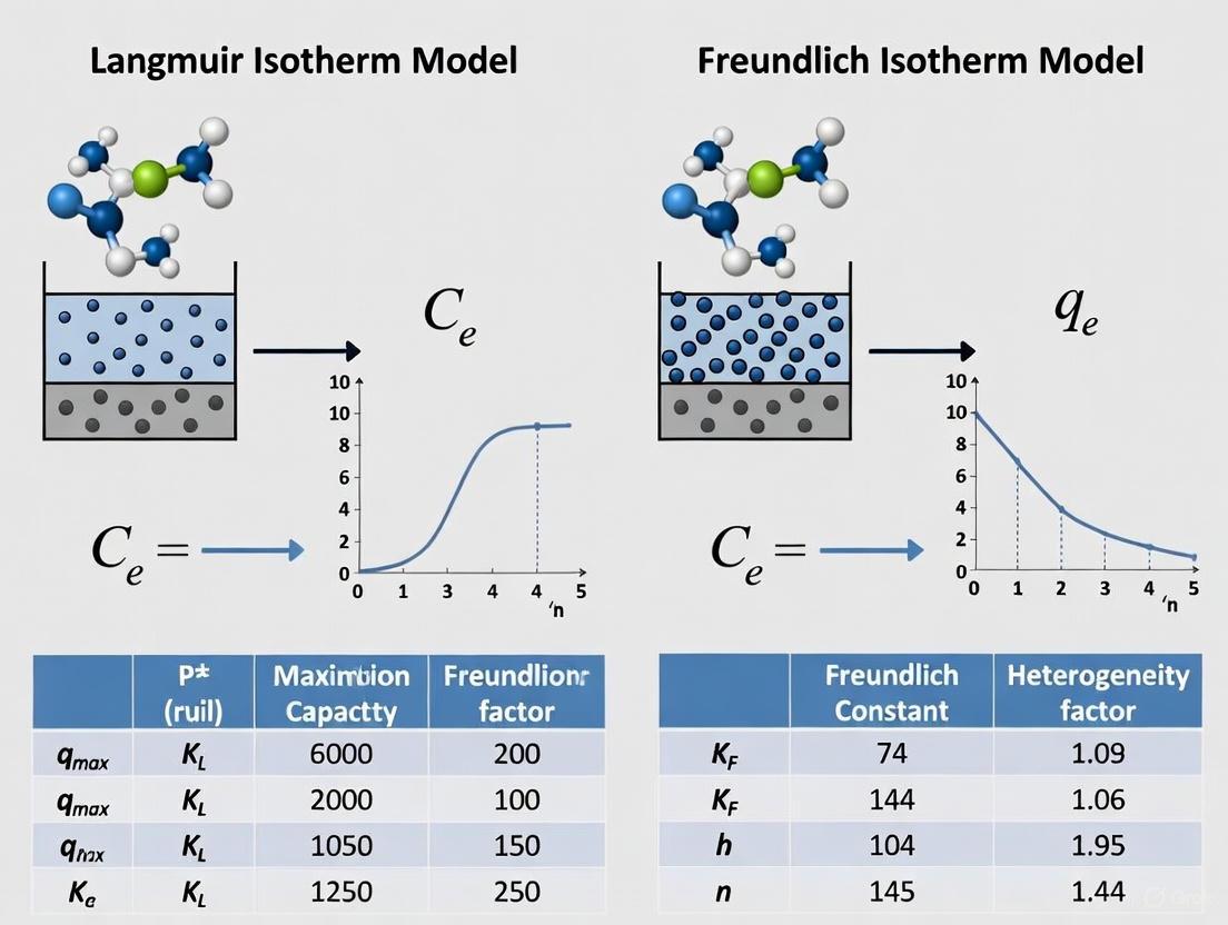
The following diagram illustrates the logical relationship between the core assumptions of each model and their mathematical forms:

Experimental Protocols for Isotherm Determination

Determining adsorption isotherms requires a systematic experimental approach to generate reliable equilibrium data. The following workflow outlines a standard batch adsorption procedure, commonly employed in both environmental and pharmaceutical sciences [1] [5].

Detailed Methodology

The standard batch adsorption experiment involves the following key steps [1] [5] [6]:

• Adsorbent Preparation and Characterization: The adsorbent (e.g., limestone, mesoporous silica, activated carbon) is often prepared, cleaned, and sieved to a specific particle size range. For synthetic materials like mesoporous silica cocoons (MSNCs), this involves a synthesis process followed by calcination at high temperature (e.g., 550°C for 6 hours) to remove the template agent. Critical characterization includes measuring the specific surface area via the Brunauer-Emmett-Teller (BET) method, pore size distribution via Barrett-Joyner-Halenda (BJH) analysis, and morphology via Scanning Electron Microscopy (SEM) or Transmission Electron Microscopy (TEM) [5].

• Stock Solution Preparation: A stock solution of the adsorbate (e.g., copper ions, indomethacin, loratadine) is prepared at a high concentration in an appropriate solvent (often water or methanol). Subsequent dilutions are made to create a series of initial concentrations ((C_0)) [6].

• Batch Equilibrium Experiments: A fixed mass of adsorbent (e.g., 0.01 g to 10 g/L) is added to a series of flasks containing a fixed volume (e.g., 10 mL to 100 mL) of solutions with varying initial adsorbate concentrations. The flasks are sealed and agitated in a temperature-controlled shaker for a predetermined time (often 24 hours) to ensure equilibrium is reached [1] [6].

• Phase Separation and Analysis: After reaching equilibrium, the solid adsorbent is separated from the liquid phase, typically by centrifugation (e.g., at 10,000 rpm for 20 minutes) and filtration. The equilibrium concentration ((C_e)) in the supernatant is then quantified using analytical techniques such as UV-Vis spectrophotometry (for drugs like loratadine and indomethacin) or Atomic Absorption Spectroscopy (for metal ions like copper) [1] [6].

• Data Calculation and Modeling: The amount adsorbed at equilibrium ((qe)) is calculated for each initial concentration using the formula: ( qe = \frac{(C0 - Ce) V}{m} ), where (V) is the solution volume and (m) is the adsorbent mass [1]. The resulting ((Ce), (qe)) data pairs are then fitted to the Langmuir and Freundlich isotherm equations using non-linear regression or linearized forms. The coefficient of determination ((R^2)) and error metrics like Root Mean Square Error (RMSE) are used to evaluate the goodness of fit [1] [7].

Comparative Analysis of Model Performance in Recent Research

The following tables synthesize experimental data from recent studies, highlighting the performance and parameters of the Langmuir and Freundlich models across diverse adsorption systems.

Table 1: Isotherm Model Performance in Environmental and Gas Adsorption Studies

Adsorbent	Adsorbate	Best-Fit Model	Langmuir Parameters	Freundlich Parameters	Key Findings	Ref.
Limestone	Copper (Cu²⁺)	Freundlich	a = 0.022 mg/gb = 1.46 L/mgR² = N/A	Kf = 0.010 mg/gn = 1.58 L/mgR² = High	Freundlich provided a better fit, especially at low initial metal concentrations, indicating surface heterogeneity.	[1]
Activated Carbon (from Olive Waste)	COâ‚‚	Multilayer Model*	Qm = 2.28 mol/kg	Kf = 1.32 mol/kg	A statistical physics multilayer model outperformed both classic models. n values >1 suggested multi-ion occupancy of sites.	[7]
Tropical Soils (Various Orders)	Phosphate (P)	Freundlich	Underestimated adsorption by ~40% at low P concentrations.	Kf varied with clay content and pH.	Freundlich best represented P sorption across soil orders; Langmuir failed at low concentrations.	[3]

*Note: This study introduced a more complex model but reported parameters for comparison.

Table 2: Isotherm Model Performance in Pharmaceutical and Drug Delivery Studies

Adsorbent	Adsorbate (Drug)	Best-Fit Model	Langmuir Parameters	Freundlich Parameters	Key Findings	Ref.
MgO-MSNCs	Indomethacin (IMC)	Freundlich	Qm = 0.93 μmol/m² (calculated)	Model showed better fit.	The heterogeneous drug coverage on the carrier surface was best described by the Freundlich isotherm.	[5]
Multi-Walled Carbon Nanotube	Loratadine	Langmuir	R² = 0.9841/qm = 0.228	R² = 0.9681/n = 0.259	The Langmuir isotherm had the highest correlation coefficient, suggesting a homogeneous adsorption process.	[6]
Mesoporous Silica (SBA-3)	Disulfiram	Hybrid Langmuir*	N/A	N/A	A single Langmuir model was inadequate. A hybrid model with two Langmuir terms for different silanol groups was required for an accurate fit.	[2]

*Note: This study developed a hybrid model to account for two distinct types of adsorption sites on the silica surface.

Discussion: Interpreting Model Selection and Parameters

The experimental data reveals that the choice between the Langmuir and Freundlich isotherm is not arbitrary but provides critical insight into the nature of the adsorption system.

• Surface Homogeneity vs. Heterogeneity: When the Langmuir model provides a superior fit (e.g., for Loratadine on carbon nanotubes [6]), it suggests a relatively uniform adsorbent surface with energetically equivalent sites. In contrast, the prevalence of the Freundlich model across most studies—from copper on limestone [1] and indomethacin on MgO-MSNCs [5] to phosphate on diverse soils [3]—highlights that surface heterogeneity is the rule rather than the exception in real-world systems. The n parameter in the Freundlich model is particularly informative; a value between 1 and 10 indicates a favorable adsorption process [1].

• Limitations and Advanced Modeling: The failure of the simple Langmuir model for complex systems like disulfiram on silica [2] and COâ‚‚ on activated carbon [7] underscores its limitations. Researchers are increasingly turning to more sophisticated models, such as hybrid Langmuir (to account for discrete sets of different sites) [2] or multilayer models derived from statistical physics (to describe multi-layer formation and pore filling) [7], to achieve a more accurate representation.

• Implications for Drug Development: For pharmaceutical scientists, the isotherm model directly impacts carrier design and process optimization. A Freundlich-type adsorption, as seen with indomethacin [5], implies a non-uniform drug distribution on the carrier and the absence of a strict monolayer capacity. This knowledge is crucial for predicting drug loading efficiency and designing controlled release profiles, as the binding energy of drug molecules is not constant but decreases as loading increases.

The Scientist's Toolkit: Essential Research Reagents and Materials

The following table catalogs key materials and reagents commonly used in adsorption studies, as evidenced by the reviewed literature.

Table 3: Key Research Reagents and Materials for Adsorption Studies

Item Name	Function/Application	Example from Research
Mesoporous Silica (SBA-3, MSNCs)	High-surface-area carrier for drug delivery and catalysis.	Used as a nanocarrier for loading drugs like disulfiram and indomethacin [2] [5].
Activated Carbon (AC)	Versatile, high-surface-area adsorbent for purification and gas capture.	Derived from olive waste for COâ‚‚ adsorption studies [7].
Cetyltrimethylammonium Bromide (CTAB)	Structure-directing agent (template) for synthesizing mesoporous silica materials.	Used in the synthesis of SBA-3 silica [2].
Pluronic P123	Triblock copolymer used as a template for mesoporous material synthesis.	Used in the synthesis of mesoporous silica cocoons (MSNCs) [5].
Tetraethyl Orthosilicate (TEOS)	Common silica precursor in the sol-gel synthesis of silicate materials.	Used as a silica source for preparing SBA-3 and MSNCs [2] [5].
Multi-Walled Carbon Nanotubes (MWCNTs)	Nanostructured adsorbent with high surface area and unique chemical properties.	Used as an adsorbent for the drug Loratadine [6].
UV-Vis Spectrophotometer	Essential analytical instrument for quantifying equilibrium concentrations of adsorbates, especially organic compounds and drugs.	Used to measure Loratadine and Indomethacin concentration before and after adsorption [5] [6].
Surface Area and Porosity Analyzer	Instrument for characterizing key adsorbent properties like surface area (BET), pore volume, and pore size distribution (BJH).	Used to characterize the textural properties of SBA-3, MSNCs, and activated carbons [7] [5].
2-chloro-N-cyclobutyl-4-iodoaniline	2-Chloro-N-cyclobutyl-4-iodoaniline|
1-(2-Chlorobenzyl)azetidin-3-ol	1-(2-Chlorobenzyl)azetidin-3-ol, CAS:1133300-64-7, MF:C10H12ClNO, MW:197.66 g/mol	Chemical Reagent

The Langmuir and Freundlich isotherm models serve as foundational tools for quantifying the relationship between equilibrium concentration and surface loading. The Langmuir model, with its clear concept of monolayer saturation, is powerful for idealized, homogeneous surfaces. However, empirical evidence from environmental science, gas adsorption, and pharmaceutical research consistently demonstrates that the Freundlich model often provides a more realistic fit for complex, heterogeneous adsorbents. The choice of model is not merely statistical; it conveys fundamental information about the surface properties of the adsorbent and the mechanism of the adsorption process. Researchers must therefore base their selection on a rigorous analysis of their own experimental data, considering the possibility that more advanced, multi-parameter models may be necessary to accurately describe systems with multiple adsorption sites or complex interactions.

Adsorption isotherms are fundamental tools in surface science, describing the equilibrium distribution of adsorbate molecules between a solid surface and the surrounding fluid phase at a constant temperature. The modeling of adsorption processes is critical for designing and optimizing systems in diverse fields, including environmental remediation, drug development, catalysis, and gas separation technologies. Among the various models developed, the Langmuir and Freundlich isotherms represent two of the most widely applied frameworks for interpreting adsorption data. The Langmuir model, introduced by Irving Langmuir in 1918, is grounded in the theory of monolayer adsorption on homogeneous surfaces. In contrast, the Freundlich model is an empirical equation that describes multilayer adsorption on heterogeneous surfaces. This guide provides an objective comparison of these two foundational models, supported by experimental data and detailed protocols, to aid researchers and scientists in selecting the appropriate model for their specific adsorption systems.

Theoretical Foundations and Model Equations

The Langmuir Isotherm Model

The Langmuir model is based on a precise set of theoretical assumptions. It posits that adsorption occurs at a finite number of identical, well-defined sites on a perfectly homogeneous surface. Each site can adsorb only one molecule, resulting in a monolayer coverage with no interaction between adsorbed molecules. The model further assumes that the adsorption energy is constant across all sites and that the surface is energetically uniform.

The Langmuir isotherm equation is expressed as: [ qe = \frac{{a b Ce}}{{1 + b C_e}} ] where:

• ( q_e ) is the amount of adsorbate adsorbed per unit mass of solid (mg/g)
• ( a ) is the maximum adsorption capacity corresponding to complete monolayer coverage (mg/g)
• ( b ) is the Langmuir adsorption constant related to the energy of adsorption (L/mg)
• ( C_e ) is the equilibrium solution concentration of the adsorbate (mg/L) [1].

The Freundlich Isotherm Model

The Freundlich model is an empirical equation used to describe adsorption on heterogeneous surfaces and is applicable to multilayer adsorption. It does not assume a maximum adsorption capacity but instead models a continuous increase in adsorption with concentration, though the rate of increase diminishes.

The Freundlich isotherm is defined as: [ qe = Kf C_e^{1/n} ] where:

• ( q_e ) is the amount of adsorbate adsorbed per unit mass of solid (mg/g)
• ( K_f ) is the Freundlich adsorption constant indicative of the adsorption capacity
• ( 1/n ) is the heterogeneity factor, an empirical constant related to adsorption intensity
• ( C_e ) is the equilibrium solution concentration of the adsorbate (mg/L) [1] [8].

A logarithmic linearization is often used: ( \ln qe = \ln Kf + \frac{1}{n} \ln Ce ), which allows for easy determination of the constants ( Kf ) and ( n ) from experimental data [4].

The Langmuir-Freundlich (Sips) Isotherm Model

Recognizing the limitations of both models, a hybrid Langmuir-Freundlich isotherm was developed. This three-parameter model can describe adsorption on heterogeneous surfaces and converges to the Langmuir model at high adsorbate concentrations and to the Freundlich model at low concentrations.

The model is given by: [ qe = \frac{{q{MLF} (K{LF}Ce)^{M{LF}}}}{{1 + (K{LF}Ce)^{M{LF}}}} ] where:

• ( q_{MLF} ) is the maximum adsorption capacity (mg/g)
• ( K_{LF} ) is the equilibrium constant
• ( M_{LF} ) is a heterogeneity parameter between 0 and 1 [9].

Table 1: Comparison of Isotherm Model Equations and Parameters

Feature	Langmuir Model	Freundlich Model	Langmuir-Freundlich Model
Theoretical Basis	Theoretical, based on kinetic principles	Empirical	Semi-empirical, hybrid
Surface Assumption	Homogeneous	Heterogeneous	Heterogeneous
Adsorption Type	Monolayer	Multilayer	Monolayer on heterogeneous sites
Key Parameters	( a ) (mg/g), ( b ) (L/mg)	( K_f ), ( n )	( q{MLF} ) (mg/g), ( K{LF} ), ( M_{LF} )
Saturation Capacity	Predicts a definite saturation (( a ))	No saturation limit; infinite surface coverage	Predicts a definite saturation (( q_{MLF} ))

Experimental Comparison and Performance Data

Case Study: Copper Removal by Limestone Adsorbent

A 2019 study provides a direct experimental comparison of the Langmuir and Freundlich models for the removal of copper (Cu) from synthetic wastewater using limestone as a low-cost adsorbent. Batch adsorption studies were conducted by varying parameters such as initial metal ion concentration, particle size of limestone, and adsorbent dosage.

The experimental data were fitted to both isotherm models, and the goodness of fit was evaluated. The results are summarized below:

Table 2: Model Parameters for Copper Adsorption on Limestone [1]

Isotherm Model	Parameter	Value	Coefficient of Determination (R²)
Langmuir	( a ) (adsorption capacity)	0.022 mg/g
	( b ) (adsorption constant)	1.46 L/mg	Not explicitly stated, but described as lower than Freundlich
Freundlich	( K_f ) (adsorption capacity)	0.010 mg/g
	( n ) (heterogeneity factor)	1.58 L/mg	High R², described as a better fit

The study concluded that for this specific system—particularly at low initial concentrations of copper—the Freundlich isotherm model provided a better description of the adsorption process, as indicated by a higher coefficient of determination (R²). This suggests that the surface of the limestone adsorbent is heterogeneous, and the adsorption of copper likely involves a more complex mechanism than simple monolayer formation [1].

Case Study: Hydroquinone Adsorption on Sandstone

A 2025 study on the adsorption behavior of hydroquinone (a gelation crosslinker) on quartz and sandstone surfaces presented a contrasting finding. The researchers applied the Langmuir, Freundlich, and Temkin isotherm models to their experimental data.

The Langmuir model demonstrated superior accuracy in predicting the adsorption capacity, with an exceptionally high R² value of 0.999 at 25°C. The model predicted a maximum adsorption capacity (( q_o )) of 47.1 mg/g. This excellent fit indicates that the adsorption of hydroquinone on the relatively homogeneous quartz surface occurs via a monolayer mechanism, validating the core assumptions of the Langmuir model [10].

Case Study: COâ‚‚ Adsorption on Activated Carbon

Research on COâ‚‚ adsorption on activated carbon (AC) derived from olive waste further illustrates the model selection process. While classical models like Langmuir and Freundlich are frequently applied, a 2025 study emphasized that they often lack detailed physicochemical parameters. The study employed advanced statistical physics models to gain deeper insight, finding that a multilayer model with two energy levels best fit the experimental data. This underscores that for complex, highly porous adsorbents like activated carbon, simple models may be insufficient for a thorough mechanistic understanding, even if they provide a good empirical fit [7].

Detailed Experimental Protocol for Batch Adsorption Studies

The following workflow and protocol are synthesized from the methodologies described in the cited research, particularly the studies on copper and hydroquinone adsorption [1] [10].

Diagram 1: Batch Adsorption Experimental Workflow

Materials and Reagent Solutions

Table 3: Essential Research Reagents and Materials

Item	Function/Description	Example from Literature
Adsorbent	The solid material that accumulates adsorbate on its surface.	Limestone (3.75 mm, 5.0 mm, 9.5 mm grades) [1]; Quartz sand [10]; Activated Carbon [7].
Adsorbate	The substance to be adsorbed from the solution or gas phase.	Copper (Cu) ions in synthetic wastewater [1]; Hydroquinone (HQ) in aqueous solution [10]; COâ‚‚ gas [7].
Shaking Incubator	Provides constant temperature and agitation for batch experiments to reach equilibrium.	Used to stir quartz-HQ mixture for 24 hours [10].
Centrifuge	Separates the solid adsorbent from the liquid phase after equilibrium is reached.	Used at 6000 rpm to separate quartz particles from HQ solution [10].
Analytical Instrument (e.g., Spectrophotometer)	Quantifies the equilibrium concentration of adsorbate in the solution.	UV-Vis spectrophotometer used to determine residual HQ concentration [10].

Step-by-Step Methodology

• Adsorbate Solution Preparation: Prepare a series of aqueous solutions of the adsorbate with varying initial concentrations (e.g., from 100 mg/L to 100,000 mg/L for hydroquinone [10]). Use distilled water and ensure complete dissolution and homogeneity using a magnetic stirrer.

• Batch Equilibrium Experiments: For each initial concentration, place a known mass of the adsorbent (e.g., 20 g of quartz [10]) into a vessel containing a known volume (e.g., 100 mL) of the adsorbate solution. Seal the vessels and place them in a shaking incubator. Maintain a constant temperature and agitation speed for a sufficient duration (e.g., 24 hours [10]) to ensure equilibrium is reached. Other parameters like adsorbent particle size and dosage can be varied systematically.

• Phase Separation: After the equilibrium period, separate the solid adsorbent from the liquid phase. This is typically achieved by centrifugation (e.g., at 6000 rpm for 10 minutes [10]) followed by filtration of the supernatant to ensure no fine particles remain.

• Equilibrium Concentration Analysis: Analyze the clear supernatant to determine the equilibrium concentration (( C_e )) of the adsorbate. For metal ions or organic compounds, techniques like UV-Vis spectrophotometry are commonly used [10]. For gases, specialized equipment like a magnetic suspension balance is employed [11] [7].

• Data Calculation: Calculate the amount of adsorbate adsorbed per unit mass of adsorbent at equilibrium (( qe )) using the following equation [1] [10]: [ qe = \frac{{(C0 - Ce) V_s}}{{m}} ] where:

  • ( C_0 ) is the initial concentration of the adsorbate (mg/L)
  • ( C_e ) is the equilibrium concentration of the adsorbate (mg/L)
  • ( V_s ) is the volume of the solution (L)
  • ( m ) is the mass of the adsorbent (g)

The following decision chart synthesizes the findings from the reviewed studies to guide researchers in selecting the most appropriate isotherm model.

Diagram 2: Isotherm Model Selection Guide

The choice between the Langmuir and Freundlich isotherm models is not a matter of which is universally superior, but rather which is more appropriate for the specific adsorbent-adsorbate system under investigation.

• Use the Langmuir Model when the adsorption process is characterized by monolayer coverage on a homogeneous surface. This is often the case for chemical adsorption (chemisorption) on well-defined crystalline materials or specific, uniform active sites. The excellent fit of the Langmuir model for hydroquinone on quartz is a prime example [10]. Its parameters provide a clear physical meaning: the maximum monolayer capacity (( a )) and the affinity constant (( b )).

• Use the Freundlich Model to describe adsorption on heterogeneous surfaces where the energy of adsorption is not uniform, often leading to multilayer formation. It is particularly useful for physical adsorption (physisorption) on complex natural materials like soils, limestone, or activated carbon, especially in the low to moderate concentration range [1] [8]. The parameters ( K_f ) and ( n ) offer insights into the relative adsorption capacity and the degree of surface heterogeneity.

• Consider Hybrid or Advanced Models like the Langmuir-Freundlich (Sips) isotherm for systems exhibiting heterogeneity but also a clear saturation limit [9]. For more complex scenarios, such as the COâ‚‚ adsorption on activated carbon, statistical physics models or models accounting for multiple energy levels can provide a more profound mechanistic understanding beyond the scope of classical models [7].

Ultimately, researchers should fit their experimental data to multiple models and use statistical metrics (like R² and RMSE) alongside a fundamental understanding of their system's physics and chemistry to select the most representative and useful adsorption isotherm.

In the field of adsorption science, researchers and industry professionals rely on mathematical models to describe how molecules interact with solid surfaces. Two of the most fundamental approaches are the Langmuir and Freundlich isotherm models, which form the theoretical basis for applications ranging from environmental remediation to pharmaceutical development. The Langmuir isotherm represents a theoretical model based on kinetic principles that describes monolayer adsorption onto a homogeneous surface, while the Freundlich isotherm serves as an empirical model for heterogeneous surfaces. Understanding their core assumptions, mathematical formulations, and experimental validity is crucial for selecting the appropriate model for specific research and development applications, particularly in drug development where purification processes depend on precise adsorption characterization.

Theoretical Foundations and Mathematical Formulations

The Langmuir Isotherm Model

The Langmuir isotherm was originally developed to describe gas-solid interactions but is now extensively applied to liquid-solid systems in various scientific and industrial fields. The model operates on a fundamental kinetic principle where the rate of adsorption equals the rate of desorption at equilibrium conditions, with no accumulation at the surface [12].

The underlying assumptions of the Langmuir model are [12] [13]:

• Identical Active Sites: The solid surface possesses uniform, homogeneous adsorption sites with identical energy.
• Monolayer Coverage: Each active site can adsorb only one molecule, resulting in a single layer of adsorbed molecules.
• No Molecular Interactions: Adsorbed molecules do not interact with one another.

The nonlinear form of the Langmuir equation is expressed as [12]:

[ qe = \frac{qo KL Ce}{1 + KL Ce} ]

Where:

• ( q_e ) = amount of adsorbate adsorbed per unit mass of adsorbent at equilibrium (mg/g)
• ( q_o ) = maximum monolayer adsorption capacity (mg/g)
• ( K_L ) = Langmuir constant related to adsorption energy (L/mg)
• ( C_e ) = equilibrium concentration of adsorbate in solution (mg/L)

The linearized form is represented as [12]:

[ \frac{Ce}{qe} = \frac{1}{KL qo} + \frac{Ce}{qo} ]

Table 1: Parameters of the Langmuir Isotherm Model

Parameter	Symbol	Units	Physical Significance
Maximum Adsorption Capacity	( q_o )	mg/g	Theoretical maximum monolayer coverage
Langmuir Constant	( K_L )	L/mg	Affinity between adsorbate and adsorbent
Equilibrium Concentration	( C_e )	mg/L	Unadsorbed concentration at equilibrium
Separation Factor	( R_L )	Dimensionless	Indicates favorability of adsorption

A key diagnostic parameter derived from the Langmuir model is the separation factor (( R_L )), defined as [12]:

[ RL = \frac{1}{1 + KL C_o} ]

Where ( Co ) is the initial concentration. The value of ( RL ) indicates the nature of the adsorption process: irreversible (( RL = 0 )), favorable (( 0 < RL < 1 )), linear (( RL = 1 )), or unfavorable (( RL > 1 )).

The Freundlich Isotherm Model

In contrast to Langmuir's theoretical approach, the Freundlich isotherm is an empirical model derived to describe multilayer adsorption on heterogeneous surfaces with sites of varying energies [14]. This model does not assume a theoretical maximum adsorption capacity, making it particularly useful for systems where adsorption capacity continues to increase with concentration.

The Freundlich equation is expressed as [1] [14]:

[ qe = KF C_e^{1/n} ]

Where:

• ( q_e ) = amount of adsorbate adsorbed per unit mass of adsorbent at equilibrium (mg/g)
• ( K_F ) = Freundlich constant indicating adsorption capacity
• ( 1/n ) = heterogeneity factor indicating adsorption intensity
• ( C_e ) = equilibrium concentration of adsorbate in solution (mg/L)

The linearized form is obtained by taking logarithms:

[ \log qe = \log KF + \frac{1}{n} \log C_e ]

Table 2: Parameters of the Freundlich Isotherm Model

Parameter	Symbol	Units	Physical Significance
Adsorption Capacity	( K_F )	mg/g	Relative adsorption capacity
Heterogeneity Factor	( 1/n )	Dimensionless	Indicator of surface heterogeneity
Adsorption Intensity	( n )	Dimensionless	Favorability of adsorption

The value of ( n ) indicates the favorability of adsorption, with values between 1 and 10 representing favorable adsorption conditions. As ( n ) increases, the adsorption intensity becomes more favorable.

Experimental Comparison: Copper Removal by Limestone Adsorbent

Methodology and Experimental Protocol

A comprehensive study comparing the applicability of Langmuir and Freundlich models was conducted using limestone as a low-cost adsorbent for copper removal from aqueous solutions [1]. The experimental protocol included the following key steps:

Materials Preparation:

• Limestone samples were obtained from two geographical sources: western red (3.75 mm diameter) and northern white (5.0 mm and 9.5 mm diameters)
• Chemical characterization showed the limestone contained primarily CaO (52.35%), with significant amounts of SiOâ‚‚ (3.15%) and LOI (43.20%)
• Samples were prepared using sieve analysis to ensure consistent particle size distribution

Batch Adsorption Studies:

• Synthetic copper solutions with varying initial concentrations (( C_o )) were prepared
• Experiments investigated parameters including initial metal ion concentration, particle size, adsorbent dosage, and equilibrium concentration
• The effects of these parameters on copper removal efficiency were systematically evaluated

Analytical Procedure:

• Known masses of limestone adsorbent were added to copper solutions
• The mixture was agitated until equilibrium was established
• Post-adsorption copper concentrations were measured to determine removal efficiency using:

[ \text{Sorption Efficiency} = \frac{C0 - Ce}{C_0} \times 100\% ]

[ qe = (C0 - C_e) \times \frac{v}{m} ]

Where ( v ) = volume of solution (L) and ( m ) = mass of adsorbent (g)

Isotherm Modeling:

• Experimental data were fitted to both Langmuir and Freundlich models
• Model parameters were determined through regression analysis
• Goodness-of-fit was evaluated using coefficient of determination (R²)

Comparative Results and Model Performance

The experimental results demonstrated that the Freundlich isotherm model provided a better fit for copper adsorption on limestone compared to the Langmuir model, particularly at lower initial copper concentrations [1].

Table 3: Experimental Parameters for Copper Adsorption on Limestone

Parameter	Langmuir Model	Freundlich Model
Adsorption Constant	( b = 1.46 ) L/mg	( K_F = 0.010 ) mg/g
Capacity Constant	( a = 0.022 ) mg/g	( n = 1.58 ) L/mg
Empirical Constant	Not applicable	( 1/n = 0.633 )
Coefficient of Determination (R²)	Lower than Freundlich	Higher than Langmuir

The Freundlich model's superior performance, indicated by higher R² values, suggests that limestone surfaces exhibit heterogeneous adsorption sites with varying energies, contrary to the homogeneous site assumption of the Langmuir model. The observed value of ( n = 1.58 ) (( n > 1 )) indicates favorable adsorption conditions for copper on limestone.

The maximum adsorption capacity of limestone for copper removal was determined to be 3.58 mg/g, demonstrating its technical feasibility as a low-cost adsorbent for wastewater treatment applications [1].

Research Applications and Practical Implications

The Scientist's Toolkit: Essential Materials for Adsorption Studies

Table 4: Essential Research Reagents and Materials for Adsorption Studies

Material/Reagent	Function in Adsorption Studies	Application Example
Activated Carbon	High-surface-area adsorbent for contaminant removal	Removal of arsenic and fluoride from water [15]
Limestone	Low-cost adsorbent for heavy metal removal	Copper removal from aqueous solutions [1]
Silica Gel	Desiccant for moisture control	Humidity control in medicines and packaging [14]
Animal Charcoal	Decolorizing agent	Removal of coloring agents from cane juice [14]
Chitosan	Biopolymer adsorbent	Removal of Fe(II) from aqueous media [1]
Bentonite Clay	Natural clay adsorbent	Removal of Zn²⁺ from wastewater [1]
2-Chloro-5-nitro-4-phenylpyridine	2-Chloro-5-nitro-4-phenylpyridine	2-Chloro-5-nitro-4-phenylpyridine is a high-purity chemical building block For Research Use Only (RUO). It is a key intermediate for synthesizing pharmaceuticals and other complex molecules. Not for human or veterinary use.
2-Phenylquinoline-7-carbaldehyde	2-Phenylquinoline-7-carbaldehyde|CAS 867162-43-4

Decision Framework for Model Selection

The choice between Langmuir and Freundlich models depends on the specific characteristics of the adsorption system and the study objectives:

Langmuir Model is preferable when:

• The surface is known to be homogeneous with uniform adsorption sites
• Monolayer coverage is expected
• Determining maximum adsorption capacity is essential
• Studying gas-solid phase interactions [12]

Freundlich Model is preferable when:

• The surface is heterogeneous with sites of different energies
• Multilayer adsorption is suspected
• Empirical correlation is sufficient for practical applications
• Working with liquid-solid systems with complex interactions [1]

For complex systems involving multiple adsorbates, extended models such as the Extended Langmuir-Freundlich (ELF) model have shown excellent fit for binary adsorption systems, as demonstrated in studies of simultaneous arsenic and fluoride removal [15].

The Langmuir and Freundlich isotherm models represent fundamentally different approaches to characterizing adsorption systems. The Langmuir model provides a theoretical foundation based on specific assumptions of uniform sites, monolayer coverage, and no intermolecular interactions. In contrast, the Freundlich model offers empirical flexibility for heterogeneous surfaces. Experimental evidence from copper removal studies on limestone demonstrates that the Freundlich model often provides better fit for real-world adsorption systems, highlighting the inherent surface heterogeneity of natural adsorbents. Researchers and drug development professionals should consider these fundamental differences when selecting appropriate models for their specific applications, with Langmuir suitable for well-characterized homogeneous surfaces and Freundlich more applicable to complex, heterogeneous systems.

In the field of separation science and environmental engineering, adsorption isotherms are fundamental tools for quantifying how molecules distribute between a solid surface and a surrounding fluid phase. For researchers and drug development professionals, selecting the appropriate adsorption model is critical for predicting compound behavior in systems ranging from water purification to pharmaceutical formulation. Two of the most prevalent models—the Langmuir and Freundlich isotherms—offer fundamentally different approaches to characterizing these interactions. The Langmuir model provides a theoretical framework based on homogeneous surface binding, while the Freundlich model offers an empirical approach specifically designed for heterogeneous surfaces with varied adsorption energies. This guide provides an objective comparison of these models' performance, supported by experimental data and detailed protocols to inform research design and interpretation.

The Freundlich model, introduced by Herbert Freundlich in 1909, has established itself as a powerful empirical tool for modeling adsorption on complex, energetically diverse surfaces commonly encountered in real-world materials such as activated carbons, soils, and bio-sorbents [16]. Unlike theoretically derived models, its empirical nature allows it to flexibly describe adsorption behavior across many heterogeneous systems where multiple simultaneous adsorption processes occur [17]. Understanding the strengths, limitations, and appropriate application contexts for both Freundlich and Langmuir models enables scientists to make informed decisions in adsorptive process design and interpretation.

Theoretical Foundations and Mathematical Formulations

The Freundlich Isotherm Model

The Freundlich isotherm expresses the relationship between the concentration of a solute adsorbed onto a solid surface and its concentration in the surrounding solution at equilibrium. Its mathematical form is:

[ qe = KF \cdot C_e^{1/n} ]

Where:

• ( q_e ) is the amount of adsorbate adsorbed per unit mass of adsorbent (mg/g)
• ( C_e ) is the equilibrium concentration of the adsorbate in solution (mg/L)
• ( K_F ) is the Freundlich constant related to adsorption capacity ((mg/g)/(mg/L)(^n))
• ( 1/n ) is the heterogeneity factor indicating adsorption intensity (dimensionless) [16] [18]

The model is particularly valuable for characterizing non-ideal sorption on heterogeneous surfaces and multilayer adsorption [19]. The parameter ( 1/n ) provides quantitative insight into the energy distribution of adsorption sites. When ( 1/n = 1 ), the adsorption is linear and site energies are uniform; as ( 1/n ) decreases below 1, the surface becomes more heterogeneous, with high-energy sites being occupied first followed by progressively lower-energy sites [17]. Typically, ( 1/n ) values range from 0.7 to 1.0 for most systems, though values outside this range occur in specific applications [17].

The Langmuir Isotherm Model

In contrast to the empirical Freundlich approach, the Langmuir model derives from theoretical assumptions about the adsorption process:

[ qe = \frac{qm \cdot KL \cdot Ce}{1 + KL \cdot Ce} ]

Where:

• ( q_m ) is the maximum adsorption capacity corresponding to complete monolayer coverage (mg/g)
• ( K_L ) is the Langmuir constant related to the energy of adsorption (L/mg)
• ( C_e ) is the equilibrium concentration of the adsorbate in solution (mg/L) [19] [18]

The Langmuir model assumes a homogeneous surface with identical adsorption sites, monolayer coverage where no further adsorption occurs once a site is occupied, and no interactions between adsorbed molecules [18] [20]. These constraints make it particularly suitable for modeling chemical adsorption (chemisorption) on uniform surfaces where binding occurs through specific chemical interactions [20].

Comparative Analysis: Model Performance and Applications

Direct Comparison of Model Parameters

Table 1: Key Characteristics of Freundlich and Langmuir Isotherm Models

Feature	Freundlich Model	Langmuir Model
Theoretical Basis	Empirical	Theoretical
Surface Assumption	Heterogeneous	Homogeneous
Adsorption Layer	Multilayer possible	Monolayer only
Site Energy	Distributed	Uniform
Saturation Capacity	No maximum predicted	Distinct maximum (qm)
Linearity Form	log qe = log KF + (1/n) log Ce	Ce/qe = 1/(KLqm) + Ce/qm
Best Application Range	Moderate concentration range	Low to high concentration
Common Applications	Environmental systems, soils, complex sorbents	Gas adsorption, engineered surfaces, specific binding

Interpretation of Model Parameters

The parameters derived from each model provide distinct insights into the adsorption process:

Freundlich Parameters:

• ( K_F ): Represents the adsorption capacity at a unit equilibrium concentration. Higher values indicate greater overall adsorption potential [20].
• ( 1/n ): Reflects the surface heterogeneity and adsorption intensity. Values between 0.7-1.0 indicate favorable adsorption, while values below 0.7 suggest highly heterogeneous surfaces with strong initial binding [17].

Langmuir Parameters:

• ( q_m ): The theoretical maximum adsorption capacity, representing complete monolayer coverage [19] [18].
• ( K_L ): Related to the affinity of binding sites and energy of adsorption. Higher values indicate stronger adsorbate-adsorbent interactions [19].

Performance in Experimental Systems

Experimental studies directly comparing both models reveal context-dependent performance:

In copper removal using limestone adsorbent, the Freundlich model demonstrated superior correlation with experimental data compared to the Langmuir model, particularly at lower contaminant concentrations [1]. The Freundlich constants reported were ( K_F = 0.010 ) mg/g and ( n = 1.58 ), with high coefficient of determination (R²) values [1].

For adsorption of orthophosphate onto oyster shell powder, the Freundlich equation provided a better mathematical description of the adsorption equilibrium than the Langmuir equation [19]. Conversely, methylene blue adsorption onto powdered activated carbon (PAC) was better described by the Langmuir model, reflecting the more homogeneous nature of the activated carbon surface for this specific adsorbate [19].

These results highlight how material properties and system conditions dictate model suitability, with Freundlich generally excelling for complex, natural adsorbents and Langmuir performing better with engineered, uniform surfaces.

Experimental Protocols and Data Analysis

Batch Adsorption Methodology

Table 2: Essential Research Reagents and Materials for Adsorption Studies

Material/Reagent	Specifications	Primary Function in Experiment
Adsorbent	Varies by study (e.g., activated carbon, limestone, oyster shell powder)	Solid surface for adsorbate attachment
Adsorbate	Target compound (e.g., heavy metals, organic dyes, pharmaceuticals)	Substance whose adsorption is being quantified
Background Electrolyte	NaCl, KCl, or CaCl2 solutions	Maintains constant ionic strength
pH Buffer Solutions	Appropriate buffer systems for target pH range	Controls solution acidity/alkalinity
Analytical Instrumentation	UV-Vis spectrophotometer, AAS, HPLC	Quantifies adsorbate concentration

A standardized batch adsorption protocol involves the following steps:

• Adsorbent Preparation: Characterize and prepare the adsorbent material with defined particle size. For example, in limestone adsorption studies, particles are typically sieved to 3.75 mm for optimal performance [1].

• Adsorbate Solution Preparation: Prepare stock solutions of known concentrations using analytical grade reagents. For heavy metal studies, solutions are often prepared from metal salts like CuSOâ‚„ or Naâ‚‚HPOâ‚„ in deionized water [19].

• Batch Equilibrium Experiments: Combine fixed masses of adsorbent (e.g., 0.1-10 g/L) with adsorbate solutions of varying initial concentrations in sealed containers. Agitate continuously in a temperature-controlled environment until equilibrium is reached (typically 24 hours) [19] [1].

• Sampling and Analysis: After reaching equilibrium, separate the solid and liquid phases by centrifugation or filtration. Analyze the supernatant for equilibrium concentration (C_e) using appropriate analytical methods [1].

• Data Calculation: Calculate adsorption capacity (q_e) using the mass balance equation:

[ qe = \frac{(C0 - C_e) \cdot V}{m} ]

Where Câ‚€ is the initial concentration (mg/L), V is the solution volume (L), and m is the adsorbent mass (g) [1].

Model Fitting and Validation

To fit experimental data to the Freundlich model, linearize the equation by taking logarithms:

[ \log qe = \log KF + \frac{1}{n} \log C_e ]

Plot log q_e versus log C_e to obtain a straight line where the intercept gives log K_F and the slope provides 1/n [16] [18]. The coefficient of determination (R²) indicates the goodness of fit, with values closer to 1.0 representing better correlation [17].

For the Langmuir model, linearize using the form:

[ \frac{Ce}{qe} = \frac{1}{KL \cdot qm} + \frac{Ce}{qm} ]

Plot C_e/q_e versus C_e to determine 1/(K_Lq_m) from the intercept and 1/q_m from the slope [19] [18].

Diagram 1: Adsorption Isotherm Model Selection Workflow. This flowchart illustrates the decision process for selecting and validating adsorption models based on experimental data.

Limitations and Advanced Modeling Approaches

Model Constraints and Considerations

Both models have specific limitations that researchers must consider:

Freundlich Model Limitations:

• Purely empirical nature provides limited mechanistic insight [18]
• Does not predict an adsorption maximum, implying infinite capacity with increasing concentration [18] [20]
• Applicability is typically restricted to moderate concentration ranges [20]
• Parameters are system-specific and cannot be extrapolated beyond tested conditions [21]

Langmuir Model Limitations:

• Assumptions of homogeneity and monolayer coverage rarely hold for complex real-world adsorbents [18]
• Cannot describe multilayer adsorption (physisorption) commonly observed in environmental systems [20]
• Fails to account for interactions between adsorbed molecules [18]
• Often requires data resolution into multiple linear regions for heterogeneous surfaces, complicating interpretation [18]

Integrated and Advanced Modeling Approaches

To address the limitations of individual models, researchers have developed several advanced approaches:

The Langmuir-Freundlich (Sips) isotherm combines features of both models:

[ qe = \frac{q{MLF} \cdot (K{LF} \cdot Ce)^{M{LF}}}{1 + (K{LF} \cdot Ce)^{M{LF}}} ]

This hybrid model behaves like the Freundlich isotherm at low concentrations and approaches Langmuir behavior at high concentrations, thus predicting monolayer capacity while accommodating surface heterogeneity [9]. The parameter M_LF (between 0 and 1) quantifies system heterogeneity [9].

Statistical analysis packages such as Statistica, Matlab, and specialized applications like IZO provide sophisticated tools for nonlinear regression analysis of adsorption data, enabling more accurate parameter estimation than traditional linearization methods [20]. These tools help researchers select the most appropriate model based on statistical goodness-of-fit metrics rather than visual assessment alone.

The Freundlich isotherm remains an indispensable tool for characterizing adsorption on heterogeneous surfaces commonly encountered in environmental systems, soils, and complex biological materials. Its empirical parameters effectively describe non-ideal behavior across moderate concentration ranges, though researchers should acknowledge its limitation in predicting maximum adsorption capacity. The Langmuir model, while theoretically grounded, performs best with homogeneous surfaces exhibiting specific, monolayer binding behavior.

For drug development professionals and researchers, model selection should be guided by the specific adsorbent-adsorbate system and the intended application of the resulting parameters. In many practical scenarios, a sequential approach—testing both models and selecting based on statistical fit—provides the most scientifically defensible pathway. The emergence of hybrid models and sophisticated fitting algorithms continues to enhance our ability to extract meaningful parameters from adsorption data, ultimately supporting advances in pharmaceutical development, environmental remediation, and separation process optimization.

In both industrial applications and environmental science, the process of adsorption—where atoms, ions, or molecules (adsorbates) accumulate on a solid surface (adsorbent)—is a critical separation and purification technique. The accurate modeling of this process is essential for designing efficient systems, from water treatment plants to drug delivery platforms. Adsorption isotherm models are the mathematical frameworks that describe the distribution of adsorbate molecules between the liquid and solid phases at equilibrium. Within this field, the Langmuir and Freundlich isotherms represent two foundational models, each with distinct theoretical bases and applications. The Langmuir model hypothesizes a homogeneous surface with identical adsorption sites and monolayer coverage, often associated with chemisorption [22] [9]. In contrast, the Freundlich isotherm is an empirical model that describes adsorption on heterogeneous surfaces and does not assume a maximum adsorption capacity, making it highly applicable to multi-layer adsorption and physical sorption processes commonly encountered with porous materials [16] [23]. This guide provides a comparative analysis of these models, with a focused examination of the significance of the Freundlich constants.

Theoretical Framework: Langmuir vs. Freundlich Models

The Langmuir Adsorption Isotherm

Developed by Irving Langmuir in 1916, this model is theoretically derived from kinetics, thermodynamics, and statistical mechanics, assuming an adsorbate behaves as an ideal gas at isothermal conditions [24]. Its core postulates are [24] [22]:

• Monolayer Coverage: Adsorption is limited to a single molecular layer on the adsorbent surface.
• Homogeneous Surface: All adsorption sites are energetically equivalent.
• No Intermolecular Interactions: Adsorbed molecules do not interact with one another.

The model is mathematically expressed as: [ qe = \frac{qm KL Ce}{1 + KL Ce} ] where:

• ( q_e ) is the amount of adsorbate adsorbed per unit mass of adsorbent at equilibrium (mg/g)
• ( q_m ) is the maximum monolayer adsorption capacity (mg/g)
• ( K_L ) is the Langmuir constant related to the energy of adsorption (L/mg)
• ( C_e ) is the equilibrium concentration of the adsorbate in solution (mg/L) [1] [22]

A dimensionless separation factor, ( RL ), can be derived to predict the favorability of adsorption: irreversible (( RL = 0 )), favorable (( 0 < RL < 1 )), linear (( RL = 1 )), or unfavorable (( R_L > 1 )) [9].

The Freundlich Adsorption Isotherm

Proposed by Herbert Freundlich in 1909, this model is empirical, derived from experimental data rather than theoretical assumptions [16]. It is designed to handle:

• Heterogeneous Surfaces: The surface of the adsorbent possesses sites with different adsorption energies.
• Multi-layer Adsorption: The model can describe adsorption beyond a single layer.

The Freundlich equation is expressed as: [ qe = KF C_e^{\,1/n} ] where:

• ( q_e ) is the amount adsorbed per unit mass of adsorbent (mg/g)
• ( C_e ) is the equilibrium concentration of the adsorbate (mg/L)
• ( K_F ) and ( n ) are the Freundlich constants specific to the adsorbate-adsorbent pair at a given temperature [16] [1] [23]

The model can also be linearized for easier parameter determination: [ \log qe = \log KF + \frac{1}{n} \log C_e ]

Table 1: Fundamental Comparison of the Langmuir and Freundlich Isotherm Models.

Feature	Langmuir Model	Freundlich Model
Theoretical Basis	Theoretical derivation	Empirical observation
Surface Nature	Homogeneous	Heterogeneous
Adsorption Layer	Monolayer	Multi-layer
Adsorption Capacity	Fixed maximum (( q_m ))	No fixed maximum; increases with ( C_e )
Constants	( qm ) (capacity), ( KL ) (affinity)	( K_F ) (capacity), ( n ) (intensity/heterogeneity)
Best Application	Chemisorption on uniform surfaces	Physisorption on porous, heterogeneous surfaces

Deep Dive into the Freundlich Constants Kf and 1/n

The utility of the Freundlich isotherm lies in the physical meaning of its two constants, which provide qualitative and quantitative insights into the adsorption process.

Kf: The Adsorption Capacity Constant

• Physical Significance: ( KF ) is an empirical constant indicative of the adsorption capacity of the adsorbent [23]. A higher value of ( KF ) generally signifies a greater adsorption capacity for the specific adsorbate under the experimental conditions. It can be visualized as the value of ( qe ) when ( Ce ) equals 1, as derived from the linearized equation.
• Dimensionality: The units of ( K_F ) are (mg/g)(L/mg)^1/n, which are dependent on the value of ( n ), making it crucial to report both constants together.

1/n: The Surface Heterogeneity and Intensity Constant

• Physical Significance: The parameter ( 1/n ) is a dimensionless measure of the deviation from linearity and the heterogeneity of the adsorption surface [16] [23].
  • If ( n = 1 ) (( 1/n = 1 )), the adsorption is linear, and the partition between the two phases is independent of concentration. This implies a relatively homogeneous surface.
  • If ( n > 1 ) (( 1/n < 1 )), it indicates that the adsorption energy decreases with increasing surface coverage. This is considered a favorable adsorption process and is characteristic of heterogeneous surfaces where the highest-energy sites are occupied first [23].
  • If ( n < 1 ) (( 1/n > 1 )), it suggests an unfavorable adsorption process, which is less common [23].
• Relationship to Heterogeneity: A value of ( 1/n ) significantly less than 1 (i.e., ( n > 1 )) is a strong indicator of surface heterogeneity. As adsorption proceeds, the adsorbate molecules fill the most favorable, high-energy sites first, and subsequently occupy less favorable sites, leading to a nonlinear isotherm curve [16].

Table 2: Interpretation of the Freundlich Constant ( n ) and its Derivative ( 1/n ).

Value of ( n )	Value of ( 1/n )	Adsorption Nature	Surface Implication
( n < 1 )	( 1/n > 1 )	Unfavorable	--
( n = 1 )	( 1/n = 1 )	Linear	Relatively homogeneous
( n > 1 )	( 1/n < 1 )	Favorable	Heterogeneous

The following diagram illustrates the logical relationship between the Freundlich constants and the properties of an adsorbent material.

Diagram 1: Logic of Freundlich constants.

Experimental Data and Model Performance Comparison

The practical performance of the Langmuir and Freundlich models varies significantly depending on the adsorbent-adsorbate system. The following table summarizes findings from recent research, highlighting the role of the Freundlich constants.

Table 3: Comparative Performance of Langmuir and Freundlich Models in Selected Studies.

Adsorbent	Adsorbate	Best-Fit Model	Freundlich Constants	Langmuir Constants	Key Finding
Limestone [1]	Copper (Cu)	Freundlich	( K_F = 0.010 ) mg/g( n = 1.58 )	( a = 0.022 ) mg/g( b = 1.46 ) L/mg	Freundlich model showed a higher coefficient of determination (R²) than Langmuir, especially at low concentrations.
Iron Oxide Impregnated Activated Carbon [25]	COâ‚‚	Freundlich	Not Specified	Not Specified	The Freundlich isotherm provided the best fit for the experimental data, confirming the heterogeneous nature of the modified adsorbent.
Various Soils [22]	Arsenic (As)	Langmuir (in most cases)	--	( q_m ) varied from 114.8 to 42,400 mg/kg across soil types	The Langmuir model, including a two-surface variant, often correlated better with soil properties like iron and clay content.

Case Study: Copper Removal by Limestone

A 2019 study provides a clear example for comparing the two models. The research aimed to remove copper ions from synthetic wastewater using limestone as a low-cost adsorbent [1].

Experimental Protocol:

• Materials: Limestone (3.75 mm, 5.0 mm, 9.5 mm particle sizes) was obtained and characterized. A synthetic copper solution was prepared.
• Batch Adsorption: Experiments were conducted by agitating a known mass of limestone adsorbent with a known volume and concentration of copper solution.
• Analysis: The effects of initial metal concentration, particle size, and adsorbent dosage were studied. After reaching equilibrium, the final concentration (( Ce )) was measured, and the amount adsorbed (( qe )) was calculated using ( qe = (C0 - C_e) \times V/m ) [1].
• Model Fitting: The (( Ce ), ( qe )) data pairs were fitted to the linear forms of both the Langmuir and Freundlich equations to determine the constants and the coefficient of determination (R²).

Result Interpretation: The Freundlich model described the process better, with ( n = 1.58 ) indicating a favorable adsorption process (( n > 1 )) on a heterogeneous surface [1]. The low value of ( K_F = 0.010 ) mg/g reflects the moderate capacity of raw limestone for copper under these specific conditions. The success of the Freundlich model suggests the limestone surface has sites with varying adsorption energies, which is expected for a natural, non-uniform material.

Essential Research Reagents and Materials

The following table lists key materials and their functions relevant to conducting adsorption experiments and analyzing data using these isotherm models.

Table 4: Research Reagent Solutions and Key Materials for Adsorption Studies.

Item	Function in Research	Example from Context
Solid Adsorbent	The material providing surface area for adsorption; its properties dictate the mechanism.	Limestone [1], Activated Carbon [25], Iron Oxide [25], Peat Moss [1], Soils [22].
Adsorbate Solution	The dissolved substance to be removed; its initial concentration is a key variable.	Copper ions [1], COâ‚‚ gas [25], Arsenic species [22].
Shaker Incubator	Provides controlled agitation and temperature to maintain isothermal conditions during batch studies.	Used in batch adsorption studies to reach equilibrium [1].
Analytical Instrument (e.g., AAS, ICP)	Quantifies the equilibrium concentration of the adsorbate in solution after adsorption.	Essential for determining ( Ce ) and subsequently ( qe ) [1].
Langmuir-Freundlich (Sips) Model	A three-parameter hybrid isotherm used for heterogeneous surfaces that approaches Langmuir behavior at high concentrations.	Resolves limitations of pure Freundlich model; useful for systems showing saturation [9].

The workflow for a typical batch adsorption study, from preparation to data analysis, is outlined below.

Diagram 2: Batch adsorption experiment workflow.

The choice between the Langmuir and Freundlich isotherm models is not a matter of one being universally superior, but rather of selecting the appropriate tool for the specific adsorbent-adsorbate system. The Langmuir model is powerful when the adsorption process is characterized by monolayer coverage on a homogeneous surface, often leading to a well-defined maximum capacity (( q_m )). In contrast, the Freundlich model excels in describing adsorption on heterogeneous surfaces, such as those of natural materials and porous carbons, where the energy of adsorption is not uniform.

For researchers, the Freundlich constants ( KF ) and ( 1/n ) provide critical, interpretable parameters. ( KF ) offers a measure of adsorption capacity, while ( 1/n ) serves as a robust indicator of surface heterogeneity and adsorption favorability. The experimental data clearly shows that for many systems, especially those involving complex, natural, or modified adsorbents, the Freundlich model provides a more accurate description of equilibrium data. Future research will continue to leverage these models, and their hybrid extensions like the Langmuir-Freundlich (Sips) isotherm, to design more efficient adsorbents for challenges ranging from environmental remediation to pharmaceutical development.

Adsorption isotherm models are fundamental tools in environmental science, chemical engineering, and pharmaceutical development for describing how solutes interact with solid surfaces. The Langmuir and Freundlich isotherms are two of the most widely used models for characterizing equilibrium adsorption data. While often applied to experimental results, these models are built on distinct theoretical foundations and core hypotheses about the nature of the adsorption process. This guide provides an objective comparison of these foundational principles, supported by experimental data and protocols, to aid researchers in selecting and applying the appropriate model for their specific adsorption system.

Core Hypotheses and Theoretical Foundations

The following table summarizes the fundamental hypotheses and characteristics of the Langmuir and Freundlich adsorption models.

Table 1: Core hypotheses and characteristics of the Langmuir and Freundlich isotherm models.

Feature	Langmuir Model	Freundlich Model
Theoretical Basis	Theoretical, derived from kinetic principles [9]	Empirical, based on experimental data fitting [3]
Surface Hypothesis	Homogeneous surface with identical adsorption sites [19] [3]	Heterogeneous surface with sites of different energies [19] [3]
Adsorption Mechanism	Monolayer adsorption: Each adsorbate molecule occupies one site; no interaction between adsorbed molecules [19] [3]	Multilayer adsorption on heterogeneous surfaces; allows for interactions [19] [3]
Energy Distribution	Constant adsorption energy, independent of surface coverage [3]	Exponentially decreasing heat of adsorption with increasing surface coverage [3]
Saturation Capacity	Predicts a clear maximum saturation capacity ((q_{max})) [19] [1]	No defined saturation limit; adsorption capacity can increase gradually [3]
Mathematical Form	( qe = \frac{q{max} KL Ce}{1 + KL Ce} ) [19]	( qe = KF C_e^{1/n} ) [1]
Key Parameters	(q{max}): Maximum adsorption capacity (mg/g)(KL): Langmuir constant related to affinity (L/mg) [1]	(K_F): Freundlich constant indicating capacity (mg/g)(n): Heterogeneity factor [1]

Experimental Protocols for Model Validation

Batch Equilibrium Adsorption Studies

The primary method for generating data to fit Langmuir and Freundlich models is the batch equilibrium experiment [26].

Workflow of a standard batch adsorption experiment to generate data for isotherm modeling.

Detailed Procedure [27] [26]:

• Solution Preparation: Prepare a series of solutions (e.g., 100 mL each) with known, varying initial concentrations ((C_0)) of the adsorbate (e.g., heavy metal, phenol, pharmaceutical compound).
• Adsorbent Addition: Add a pre-determined, fixed mass of the adsorbent (e.g., 0.1 to 1.0 g) to each solution. The adsorbent mass should be constant across all bottles to ensure the adsorbent dose is consistent [1].
• Equilibration: Seal the bottles and agitate them in a shaker incubator at a constant temperature (e.g., 25°C ± 2°C) for a predetermined period (often 24 hours) to ensure equilibrium is reached [27] [26].
• Separation: After equilibration, separate the solid adsorbent from the liquid phase using centrifugation or filtration.
• Analysis: Analyze the supernatant or filtrate to determine the equilibrium concentration of the adsorbate ((C_e)) using appropriate analytical techniques (e.g., UV-Vis spectroscopy, conductivity meter, ICP-MS) [26].
• Calculation: The amount of adsorbate adsorbed per unit mass of adsorbent at equilibrium ((qe), mg/g) is calculated using the mass balance equation: ( qe = \frac{(C0 - Ce) V}{m} ) where (V) is the volume of the solution (L), and (m) is the mass of the adsorbent (g) [1] [27].

Data Fitting and Model Selection

Once (qe) and (Ce) data pairs are obtained, they are fitted to the linear or non-linear forms of the Langmuir and Freundlich models.

Table 2: Model fitting and statistical validation approaches.

Step	Description	Purpose
Linear Regression	Transforming models to linear forms (e.g., (Ce/qe) vs. (Ce) for Langmuir; log (qe) vs. log (C_e) for Freundlich) and fitting via least squares [27].	Initial parameter estimation.
Non-Linear Regression	Fitting the raw ((Ce), (qe)) data directly to the non-linear model equations using iterative algorithms [27].	Avoids bias introduced by linearization; preferred method [27].
Error Function Analysis	Calculating statistical metrics like Sum of Squared Errors (SSE), Hybrid Fractional Error Function (HYBRID), and Marquardt’s Percent Standard Error (MPSED) [27].	Quantifies the deviation between experimental data and model predictions.
Goodness-of-Fit	Evaluating the coefficient of determination (R²) and performing Chi-square (χ²) tests [15] [27].	Determines which model provides the best fit to the experimental data.

The Scientist's Toolkit: Essential Research Reagents and Materials

Table 3: Key reagents, materials, and equipment used in adsorption isotherm studies.

Item	Function/Application	Example from Literature
Activated Carbon (PAC/GAC)	High-surface-area adsorbent for removing organic and inorganic contaminants from water [19].	Used for methylene blue adsorption [19].
Low-Cost Alternative Adsorbents	Economical and sustainable materials for wastewater treatment.	Oyster shell powder (for orthophosphate) [19], limestone (for copper removal) [1], crushed mollusk shells, peat moss [1].
Model Adsorbates	Representative compounds used to test adsorbent performance.	Methylene blue (dye), Copper/Cadmium/Nickel (heavy metals), Phenol (organic pollutant), Orthophosphate (nutrient) [19] [1] [27].
Batch Reactors	Sealed vessels (e.g., conical flasks, serum bottles) for containing the adsorbent-adsorbate mixture during equilibration [26].	Used in all batch equilibrium studies.
Analytical Instruments	Quantifies adsorbate concentration before and after adsorption.	UV-Vis Spectrophotometer (for colored ions/dyes), Conductivity Meter (for ionic species) [26], ICP-MS (for metals).
6-(2-Hydroxyethyl)-1-naphthoic acid	6-(2-Hydroxyethyl)-1-naphthoic acid, CAS:614754-39-1, MF:C13H12O3, MW:216.23 g/mol	Chemical Reagent
5-(Azidomethyl)-2-methylpyrimidine	5-(Azidomethyl)-2-methylpyrimidine|CAS 1073428-44-0	5-(Azidomethyl)-2-methylpyrimidine is a key chemical building block for research. This product is for Research Use Only and is not intended for human or veterinary use.

The choice between the Langmuir and Freundlich models is not merely a statistical exercise but a decision based on the physical and chemical nature of the adsorbent-adsorbate system. The Langmuir model is most appropriate for systems that likely involve monolayer, chemical adsorption onto a homogeneous surface with a finite capacity, such as the adsorption of methylene blue onto activated carbon [19]. In contrast, the Freundlich model is often a better fit for physical adsorption processes on heterogeneous surfaces, such as phosphate sorption in diverse tropical soils [3] or copper removal by limestone [1]. Researchers should prioritize non-linear regression coupled with robust statistical error analysis to objectively determine the model that most accurately describes their experimental data, ensuring more reliable predictions for process design and optimization.

Practical Application and Data Analysis Methodologies

The analysis of adsorption data is a fundamental process in environmental science, materials research, and pharmaceutical development, providing critical insights into the interaction between substances and surfaces. The Langmuir and Freundlich isotherm models represent two cornerstone mathematical approaches for describing these adsorption equilibria. While the Langmuir model originates from theoretical assumptions of homogeneous monolayer adsorption, the Freundlich equation serves as an empirical powerhouse for characterizing heterogeneous systems. The transformation of these models into linear forms has historically dominated experimental practice, enabling researchers to extract parameters through simple linear regression. However, advances in computational power and statistical understanding have revealed significant limitations in these linearized forms, prompting a paradigm shift toward non-linear regression techniques. This guide objectively compares the performance, application, and data fitting capabilities of both linear and non-linear implementations of these classic models, providing researchers with evidence-based protocols for selecting optimal approaches based on their specific experimental systems and research objectives.

Theoretical Foundations of Adsorption Models

Langmuir Adsorption Isotherm

The Langmuir adsorption model, developed by Irving Langmuir in 1916, hypothesizes monolayer adsorption onto a surface containing a finite number of identical binding sites [24] [22]. The model operates under several key assumptions: (1) the adsorbent surface is homogeneous and flat, (2) all adsorption sites are energetically equivalent, (3) each site can accommodate only one adsorbate molecule, (4) no interactions occur between adsorbed molecules, and (5) adsorption is reversible [24] [18]. These assumptions create an idealized system where the energy of adsorption is constant across all sites and independent of surface coverage.

The fundamental Langmuir equation is expressed as:

[ qe = \frac{qm \cdot KL \cdot Ce}{1 + KL \cdot Ce} ]

Where:

• ( q_e ) = amount of adsorbate adsorbed per unit mass of adsorbent at equilibrium (mg/g)
• ( q_m ) = maximum adsorption capacity corresponding to complete monolayer coverage (mg/g)
• ( K_L ) = Langmuir constant related to adsorption energy (L/mg)
• ( C_e ) = equilibrium concentration of adsorbate in solution (mg/L) [1] [22]

The model finds particular relevance in systems where chemical adsorption dominates and surface homogeneity can be reasonably assumed. Its ability to predict a maximum adsorption capacity (( q_m )) makes it invaluable for estimating the theoretical limits of adsorption systems in water treatment and pharmaceutical applications.

Freundlich Adsorption Isotherm

In contrast to the theoretically-derived Langmuir model, the Freundlich isotherm emerged as an empirical relationship to describe adsorption behavior on heterogeneous surfaces [18] [16]. First proposed by Herbert Freundlich in 1909, this model does not assume a maximum adsorption capacity but rather describes multilayer adsorption with a distribution of binding site energies.

The fundamental Freundlich equation is expressed as:

[ qe = KF \cdot C_e^{1/n} ]

Where:

• ( q_e ) = amount of adsorbate adsorbed per unit mass of adsorbent at equilibrium (mg/g)
• ( K_F ) = Freundlich constant indicative of adsorption capacity (mg/g)
• ( 1/n ) = heterogeneity factor representing adsorption intensity (dimensionless)
• ( C_e ) = equilibrium concentration of adsorbate in solution (mg/L) [1] [18] [16]

The Freundlich model particularly excels in describing adsorption on complex, heterogeneous surfaces like soils, activated carbon, and biological materials. The parameter ( 1/n ) provides valuable information about adsorption favorability: values between 0.1 and 1.0 indicate favorable adsorption, while values closer to zero suggest greater surface heterogeneity [18] [17]. Unlike the Langmuir model, Freundlich does not predict saturation of the surface, making it more applicable across wider concentration ranges for many real-world systems.

Linear versus Non-Linear Data Fitting Approaches

Linear Transformation Methods

The transformation of non-linear isotherm equations into linear forms has been historically prevalent due to computational simplicity and accessibility. These linearizations allow researchers to extract parameters using basic linear regression techniques, but each transformation introduces specific statistical distortions.

Table 1: Linear Forms of Langmuir and Freundlich Isotherm Equations

Isotherm Model	Linear Form	Plot Type	Parameters from Plot	Common Limitations
Langmuir	( \frac{Ce}{qe} = \frac{1}{KL \cdot qm} + \frac{Ce}{qm} )	( Ce/qe ) vs ( C_e )	Slope = ( 1/qm ), Intercept = ( 1/(KL \cdot q_m) )	Overemphasizes low-concentration data; distorts error structure
Langmuir	( \frac{1}{qe} = \frac{1}{qm} + \frac{1}{KL \cdot qm} \cdot \frac{1}{C_e} )	( 1/qe ) vs ( 1/Ce )	Slope = ( 1/(KL \cdot qm) ), Intercept = ( 1/q_m )	Overemphasizes high-concentration data; poor at low concentrations
Freundlich	( \log qe = \log KF + \frac{1}{n} \log C_e )	( \log qe ) vs ( \log Ce )	Slope = ( 1/n ), Intercept = ( \log K_F )	Alters error distribution; biases parameter estimates

The linear Langmuir form (( Ce/qe ) vs ( Ce )) remains the most widely used linearization, providing ( qm ) from the slope and ( K_L ) from the intercept [22]. Similarly, the logarithmic Freundlich transformation enables straightforward parameter estimation through linear regression of log-transformed data [18] [16]. However, these linearizations fundamentally alter error distribution and weighting across the data range. The logarithmic transformation particularly compresses the error structure, giving unequal weight to data points and potentially biasing parameter estimates [17].

Non-Linear Regression Approach

Non-linear regression techniques fit model parameters directly to the untransformed data, maintaining the intrinsic error structure and providing statistically superior parameter estimates. This approach minimizes the sum of squared residuals between observed and predicted ( q_e ) values using iterative computational algorithms.

The fundamental non-linear equations are:

Langmuir non-linear form: [ qe = \frac{qm \cdot KL \cdot Ce}{1 + KL \cdot Ce} ]

Freundlich non-linear form: [ qe = KF \cdot C_e^{1/n} ]

Non-linear fitting preserves the homoscedastic nature of experimental errors (assuming constant variance in ( q_e )) and provides unbiased parameter estimates with more realistic confidence intervals. Modern statistical software packages (R, Python SciPy, Origin, GraphPad Prism) have made non-linear regression accessible to researchers across disciplines. The direct fitting approach also allows for more sophisticated model comparison using information-theoretic approaches like Akaike Information Criterion (AIC), enabling objective selection between competing models based on their ability to explain data with minimal parameters.

Comparative Performance in Experimental Systems

Direct comparisons of linear and non-linear fitting approaches reveal significant differences in parameter estimation and model accuracy. A study on copper removal by limestone adsorbent demonstrated that the Freundlich model provided better fit to experimental data compared to the Langmuir model, with the non-linear approach accurately capturing the adsorption behavior across varying initial concentrations [1]. The Freundlich parameters obtained were ( K_F = 0.010 ) mg/g and ( n = 1.58 ) l/mg, with high coefficient of determination [1].

Table 2: Comparison of Isotherm Model Performance in Experimental Systems

Adsorption System	Best-Fitting Model	Model Parameters	Coefficient of Determination (R²)	Reference
Copper on limestone	Freundlich (non-linear)	( K_F = 0.010 ) mg/g, ( n = 1.58 )	High R²	[1]
Hydroquinone on carbonate rocks	Langmuir (non-linear)	( qm = 45.2 ) mg/g (25°C), ( KL = 0.243 ) L/mg	R² = 0.99	[28]
Arsenic on activated carbon	Modified Langmuir-Freundlich	Combined parameters	R² = 0.99	[15]

For hydroquinone adsorption on carbonate rocks, the Langmuir model demonstrated excellent fit with non-linear regression, revealing temperature-dependent parameters with ( q_m ) decreasing from 45.2 mg/g at 25°C to 34.2 mg/g at 90°C [28]. The spontaneous and exothermic nature of the process was confirmed through thermodynamic analysis [28]. In complex multi-component systems, modified models like the Extended Langmuir-Freundlich have shown superior performance for simultaneous adsorption of arsenic and fluoride on activated carbon, with R² values of 0.99 and minimal error metrics [15].

Experimental Protocols and Methodologies

Standard Batch Adsorption Experiments

Batch adsorption experiments represent the fundamental methodology for generating isotherm data across research disciplines. The following protocol outlines the standardized approach for collecting high-quality adsorption data suitable for both Langmuir and Freundlich analysis:

• Adsorbate Solution Preparation: Prepare a series of adsorbate solutions across appropriate concentration ranges (e.g., 10-500 mg/L for organic compounds, 10-200 mg/L for heavy metals). Use analytical grade reagents and deionized water to minimize interference [1] [28].

• Adsorbent Characterization: Characterize the adsorbent material for particle size distribution, specific surface area (BET method), porosity, and surface functional groups (FTIR). For limestone adsorbents, typical effective sizes range from 3.75 mm to 9.5 mm, with chemical composition primarily calcite (>95%) [1] [28].

• Equilibrium Studies: In separate containers (typically 250 mL Erlenmeyer flasks), combine fixed adsorbent doses (e.g., 0.1-2.0 g) with varying initial concentrations of adsorbate solution. Maintain constant solution volume (e.g., 100 mL) across all samples [1].

• Agitation and Equilibrium: Agitate the mixtures in a temperature-controlled shaker at constant speed (e.g., 150 rpm) until equilibrium is reached (typically 24 hours for aqueous systems, confirmed through preliminary kinetic studies) [1].

• Separation and Analysis: Separate the adsorbent from solution by centrifugation (e.g., 4000 rpm for 10 minutes) and filtration (0.45 μm membrane filters). Analyze the supernatant for residual adsorbate concentration using appropriate analytical techniques (UV-Vis spectroscopy, AAS, HPLC, depending on the adsorbate) [1].

• Data Calculation: Calculate the amount adsorbed at equilibrium (( qe )) using the mass balance equation: [ qe = \frac{(C0 - Ce) \cdot V}{m} ] Where ( C0 ) = initial concentration (mg/L), ( Ce ) = equilibrium concentration (mg/L), V = solution volume (L), and m = adsorbent mass (g) [1].

Model Fitting and Validation Procedures

Once experimental ( qe ) and ( Ce ) data pairs are obtained, systematic fitting procedures should be implemented:

• Non-Linear Regression Protocol:

  • Input experimental (( Ce ), ( qe )) data pairs directly into statistical software
  • Define the isotherm equation with appropriate parameters
  • Implement iterative algorithms (Levenberg-Marquardt typically provides robust convergence)
  • Set appropriate parameter constraints (( qm > 0 ), ( KL > 0 ), ( K_F > 0 ), ( n > 0 ))
  • Use uniform weighting unless heteroscedasticity is confirmed
  • Record parameter estimates with 95% confidence intervals

• Linear Regression Protocol:

  • Transform data according to desired linear form (see Table 1)
  • Perform ordinary least squares regression on transformed data
  • Back-calculate original parameters from slope and intercept
  • Calculate determination coefficient (R²) for linearized data

• Model Validation Metrics:

  • Calculate multiple error functions: Root Mean Square Error (RMSE), Normalized Average Percentage Error (NAPE), and Akaike Information Criterion (AIC) for model comparison [15]
  • Perform residual analysis to identify systematic trends
  • Compare adjusted R² values for models with different parameter numbers
  • Validate with additional experimental data not used in fitting

Figure 1: Experimental workflow for adsorption studies and model fitting

Advanced Modeling Considerations

Modified and Competitive Adsorption Models

Real-world applications often involve complex systems requiring advanced modeling approaches beyond the basic Langmuir and Freundlich equations. When dealing with multiple adsorbates or heterogeneous surfaces, researchers should consider these enhanced models:

Two-Surface Langmuir Model: Accounts for two distinct types of adsorption sites with different energies: [ qe = \frac{K{L1} \cdot q{m1} \cdot Ce}{1 + K{L1} \cdot Ce} + \frac{K{L2} \cdot q{m2} \cdot Ce}{1 + K{L2} \cdot C_e} ] This model has successfully described arsenic adsorption on soils, where high-energy and low-energy surfaces represent different mineral phases [22].

Extended Langmuir-Freundlich (ELF) Model: Combines features of both models for multi-component systems: [ q{e,i} = \frac{q{m,i} \cdot (K{L,i} \cdot C{e,i})^{ni}}{1 + \sum{j=1}^N (K{L,j} \cdot C{e,j})^{n_j}} ] This model demonstrated excellent fit (R² = 0.99) for simultaneous adsorption of arsenic and fluoride on activated carbon, outperforming traditional competitive models [15].

Modified Competitive Langmuir (MCL) Model: Addresses selective adsorption in binary systems, particularly useful when one component exhibits pronounced antagonistic behavior over another, as observed with arsenic showing greater adsorption selectivity over fluoride [15].

Temperature Dependence and Thermodynamic Analysis

Adsorption processes are inherently temperature-dependent, and incorporating thermal effects provides deeper insight into adsorption mechanisms. The temperature dependence of Langmuir parameters follows Arrhenius-type behavior:

[ KL = K0 \cdot \exp\left(-\frac{\Delta H}{RT}\right) ]

Where ( \Delta H ) represents the enthalpy of adsorption. For hydroquinone on carbonate rocks, the adsorption was exothermic (( \Delta H = -6494 ) J/mol) and spontaneous across temperatures from 25-90°C, with Gibbs free energy (( \Delta G )) ranging from -8335 to -8737 J/mol [28].

The integration of temperature studies enables calculation of fundamental thermodynamic parameters:

• Gibbs Free Energy (( \Delta G )): Determines spontaneity of adsorption process
• Enthalpy (( \Delta H )): Identifies exothermic (physical) or endothermic (chemical) adsorption
• Entropy (( \Delta S )): Reflects changes in system disorder upon adsorption

These parameters collectively provide mechanistic insights beyond simple capacity measurements, distinguishing between physisorption (typically -20 to 0 kJ/mol) and chemisorption (typically -400 to -80 kJ/mol) based on the magnitude of ( \Delta H ).

Research Reagent Solutions and Materials

Table 3: Essential Research Materials for Adsorption Experiments

Material/Reagent	Specifications	Function in Experiments	Example Application
Limestone adsorbent	Particle size: 3.75-9.5 mm; Composition: >95% calcite; Low density (ASTM C568)	Porous media for heavy metal removal	Copper removal from aqueous solutions [1]
Activated carbon	BET surface area: 500-1500 m²/g; Various mesh sizes	High-surface-area adsorbent for organic compounds	Simultaneous arsenic and fluoride removal [15]
Carbonate rocks	High-purity calcite (>95%); Crushed to 2-4 μm particles	Model adsorbent for petroleum applications	Hydroquinone adsorption studies [28]
Hydroquinone	Purity: >98%; Molecular formula: C₆H₆(OH)₂	Cross-linker adsorbate for enhanced oil recovery	Adsorption on carbonate rocks [28]
Heavy metal salts	Analytical grade CuSOâ‚„, ZnClâ‚‚, etc.	Model inorganic adsorbates	Copper removal studies [1]

The comparison between linear and non-linear forms of Langmuir and Freundlich equations reveals a complex landscape where statistical rigor must be balanced against practical considerations. While linear transformations offer computational simplicity and accessibility, they introduce significant statistical artifacts through error structure modification and data weighting imbalances. Non-linear regression preserves the intrinsic error distribution and provides more accurate parameter estimates with realistic confidence intervals, making it the statistically superior approach for precise quantitative work.

Experimental evidence demonstrates that model performance is highly system-dependent. The Freundlich model excels in describing heterogeneous surfaces like soils and activated carbons, while the Langmuir model better represents monolayer adsorption on homogeneous surfaces. For complex multi-component systems, modified models like the Extended Langmuir-Freundlich equation provide enhanced fitting capabilities. The research community should prioritize non-linear fitting as the standard approach while maintaining linear methods for preliminary analysis and educational purposes. Future directions should focus on developing more sophisticated models that better capture the complexity of real adsorption systems while maintaining practical parameterizability.

Step-by-Step Guide to Calculating Langmuir Parameters (qmax and KL) from Experimental Data

In adsorption systems research, understanding how contaminants interact with solid surfaces is fundamental for developing effective purification materials, drug delivery systems, and environmental remediation technologies. The Langmuir isotherm model hypothesizes monolayer adsorption on a homogeneous surface with identical adsorbing sites, making it particularly suitable for characterizing chemisorption processes where chemical bonds form between adsorbate and adsorbent [22]. This guide provides a comprehensive, step-by-step framework for calculating the essential Langmuir parameters—maximum adsorption capacity (qmax) and Langmuir constant (KL)—from experimental data, while objectively comparing its performance with the alternative Freundlich model.

The Langmuir theory represents the first theoretically developed adsorption isotherm and retains importance in both physisorption and chemisorption studies. It is based on a kinetic viewpoint where the rate of adsorption equals the rate of desorption at dynamic equilibrium [22]. For researchers in pharmaceutical development and environmental science, accurately determining Langmuir parameters provides critical insights into binding efficiency, surface coverage, and adsorbent performance under specific experimental conditions.

Theoretical Foundations of the Langmuir Model

Core Principles and Assumptions

The Langmuir model operates on several fundamental assumptions that define its application scope:

• Monolayer Coverage: Adsorption is limited to a single molecular layer on the adsorbent surface
• Homogeneous Surface: All adsorption sites are energetically equivalent and identical
• Independent Sites: No interaction occurs between adsorbed molecules on adjacent sites
• Dynamic Equilibrium: The adsorption process reaches equilibrium when adsorption and desorption rates equalize

These assumptions make the Langmuir model particularly appropriate for characterizing chemisorption processes and systems with homogeneous binding sites [22] [20]. In drug development, this model helps quantify specific receptor-ligand interactions and binding affinities.

Mathematical Formulations

The Langmuir isotherm equation can be expressed in multiple forms, each serving different analytical purposes:

Non-linear form:

Linear form:

Where:

• q_e = amount of adsorbate adsorbed per unit mass of solid at equilibrium (mg/g)
• q_max = maximum adsorption capacity (mg/g)
• K_L = Langmuir adsorption constant related to energy of adsorption (L/mg)
• C_e = equilibrium solution concentration of adsorbate (mg/L) [22] [1]

The linear form is particularly valuable for experimental data analysis as it allows direct calculation of parameters from slope and intercept values.

Experimental Protocols for Data Generation

Batch Adsorption Studies Methodology

Generating reliable data for Langmuir parameter calculation requires meticulous experimental design. The following protocol outlines the standard batch adsorption methodology:

• Adsorbent Preparation: Characterize and prepare adsorbent material with consistent particle size. Studies show that particle size significantly impacts removal efficiency, with limestone of 3.75 mm diameter demonstrating optimal copper removal compared to larger sizes [1].

• Stock Solution Preparation: Prepare precise concentrations of adsorbate solution. For heavy metals like copper, initial concentrations (Câ‚€) typically range from 10-50 mg/L [1].

• Experimental Setup: Conduct experiments in controlled batches with varying initial concentrations while maintaining constant:

  • Adsorbent dosage (mass per volume)
  • Solution pH and temperature
  • Contact time (until equilibrium reached)
  • Agitation speed

• Equilibrium Establishment: Allow sufficient time for system equilibrium. Studies indicate adsorption capacities increase significantly with reaction time—from 92.2 mg/kg to 418.2 mg/kg for Olivier loam as contact time extended from 6 to 504 hours [22].

• Sampling and Analysis: Measure equilibrium concentration (C_e) using appropriate analytical techniques (AAS, ICP-MS, UV-Vis spectroscopy).

• Data Calculation: Calculate adsorption capacity at equilibrium (q_e) using the mass balance equation:

Where V = solution volume (L) and m = adsorbent mass (g) [1].

Research Reagent Solutions Toolkit

Table 1: Essential Research Materials for Adsorption Experiments

Reagent/Material	Function in Experiment	Specifications & Considerations
Adsorbent Material	Solid surface for adsorption	Characterize surface area, particle size, porosity
Analyte Standards	Target contaminant for study	High-purity reference materials for calibration
pH Buffer Solutions	Control solution acidity/alkalinity	Maintain consistent pH across experimental batches
Activated Carbons	Reference adsorbent material	Vary by surface chemistry (ORGANOSORB 10, DESOTEK, BA-10) [20]
Natural Adsorbents	Low-cost alternative materials	Limestone, bentonite clay, mollusk shells [1]
Analytical Instruments	Concentration measurement	AAS, ICP-MS, UV-Vis spectrophotometer
1-Benzyl-4-(4-bromophenyl)pyrazole	1-Benzyl-4-(4-bromophenyl)pyrazole, CAS:1191063-24-7, MF:C16H13BrN2, MW:313.19 g/mol	Chemical Reagent
Methoxytrityl-N-PEG12-TFP ester	Methoxytrityl-N-PEG12-TFP Ester|CAS 1334169-92-4	Methoxytrityl-N-PEG12-TFP ester is a bioconjugation reagent for amine modification. For Research Use Only. Not for human or veterinary diagnostic or therapeutic use.

Step-by-Step Calculation of Langmuir Parameters

Data Preparation and Transformation

The linearized Langmuir equation provides the most straightforward method for calculating qmax and KL:

• Compile Experimental Data: Tabulate equilibrium concentrations (Ce) and corresponding adsorption capacities (qe) from batch experiments.

• Transform Variables: Calculate Ce/qe values for each data point to prepare for linear regression.

Table 2: Sample Data Transformation for Langmuir Linearization

C_e (mg/L)	q_e (mg/g)	Ce/qe (g/L)
5.2	18.3	0.284
8.7	29.6	0.294
12.1	38.9	0.311
16.8	47.2	0.356
22.4	54.1	0.414

• Plot Linearized Data: Graph Ce/qe versus Ce. The x-axis represents Ce values, while the y-axis represents Ce/qe values.

Linear Regression and Parameter Calculation

• Perform Linear Regression: Apply least-squares regression to the transformed data points to obtain the best-fit line.

• Calculate Slope and Intercept:

  • Slope = 1/q_max
  • Intercept = 1/(KL × qmax)

• Determine Langmuir Parameters:

  • q_max = 1 / Slope
  • KL = 1 / (Intercept × qmax) = Slope / Intercept

For example, in a study on arsenic adsorption, the Langmuir model calculated qmax and KL values of 370.37 mg/g and 0.00367 L/mg, respectively [22].

Workflow Visualization

Comparative Analysis: Langmuir vs. Freundlich Models

Performance Evaluation with Experimental Data

Table 3: Direct Comparison of Langmuir and Freundlich Parameters from Limestone Copper Adsorption

Parameter	Langmuir Model	Freundlich Model
Maximum Capacity	a = 0.022 mg/g	K_f = 0.010 mg/g
Affinity Constant	b = 1.46 L/mg	n = 1.58 L/mg
Coefficient of Determination (R²)	Lower values reported	Higher values reported [1]
Best Application Scope	High concentration systems	Low initial concentrations [1]
Surface Heterogeneity	Assumes homogeneous sites	Accommodates surface heterogeneity

Model Selection Guidelines

The choice between Langmuir and Freundlich models depends on specific experimental conditions and system characteristics:

• Langmuir preferred when:

  • Surface is relatively homogeneous
  • Monolayer coverage is expected
  • Chemisorption dominates the process
  • High concentration systems are studied [22]

• Freundlich preferred when:

  • Surface is heterogeneous
  • Multilayer adsorption occurs
  • Low initial contaminant concentrations
  • Physical adsorption dominates [22] [1]

Research comparing both models for copper removal on limestone found that the "Freundlich isotherm model described the adsorption process with high coefficient of determination R², better than the Langmuir isotherm model for low initial concentration of heavy metal" [1].

Advanced Applications and Modifications

Two-Surface Langmuir Model

For heterogeneous surfaces exhibiting multiple binding site types, the standard Langmuir model may prove inadequate. In such cases, the Langmuir two-surface equation better represents the system:

Where qmax₁ and KL₁ represent low-energy surface sites, and qmax₂ and KL₂ represent high-energy surface sites [22]. This approach effectively models systems where plots of the Langmuir one-surface equation yield two straight-line portions with different gradients.

Temperature Dependence and Thermodynamics

Langmuir parameters exhibit temperature dependence, providing valuable thermodynamic insights:

• Adsorption capacity (qmax) typically increases with temperature, as seen in arsenic adsorption studies where qmax values increased from 13.22 mg/kg to 16.37 mg/kg when temperature rose from 283K to 323K [22]

• Langmuir constant (K_L) relates to adsorption energy and can be used to calculate thermodynamic parameters including Gibbs free energy, enthalpy, and entropy changes

The Langmuir model remains a fundamental tool for characterizing adsorption systems across pharmaceutical, environmental, and materials science research. By following the step-by-step calculation methodology outlined in this guide, researchers can reliably determine qmax and KL parameters that quantify adsorption capacity and affinity. While the Freundlich model may provide better fits for heterogeneous surfaces and low concentration systems, the Langmuir model excels in characterizing monolayer adsorption on homogeneous surfaces, particularly in chemisorption applications.

The selection between these models should be guided by system characteristics, with the understanding that modified Langmuir approaches (such as the two-surface model) can extend applicability to more complex systems. As adsorption research advances, particularly in multicomponent systems, these fundamental isotherm models provide the critical foundation for understanding and optimizing contaminant removal, drug delivery mechanisms, and surface interaction phenomena.

Step-by-Step Guide to Calculating Freundlich Parameters (K_f and n) from Experimental Data

The Freundlich isotherm is a crucial empirical model used to describe non-ideal adsorption on heterogeneous surfaces, representing multilayer adsorption where the adsorption energy decreases exponentially with increasing surface coverage [3]. Unlike the Langmuir model, which assumes a homogeneous surface with monolayer coverage, the Freundlich model does not predict a saturation limit, making it particularly effective for modeling adsorption across a wide range of concentrations, especially in complex systems like soils and activated carbons [3]. The model's ability to represent sorption that continues to increase as more adsorbate is added makes it highly relevant for environmental and industrial applications, from phosphorus dynamics in tropical soils to heavy metal removal from wastewater [3] [1]. Recent studies across various fields have confirmed that the Freundlich equation often provides a superior fit for experimental data compared to other isotherm models, particularly for heterogeneous surfaces commonly encountered in real-world applications [3].

Theoretical Foundation of the Freundlich Model

The Freundlich Equation

The Freundlich adsorption isotherm is mathematically expressed as:

[ qe = KF \cdot C_e^{1/n} ]

Where:

• ( q_e ) = amount of adsorbate adsorbed per unit mass of adsorbent at equilibrium (mg/g)
• ( C_e ) = equilibrium concentration of the adsorbate in solution (mg/L)
• ( K_F ) = Freundlich constant representing adsorption capacity (mg/g)(L/mg)(^{1/n})
• ( 1/n ) = empirical constant representing adsorption intensity or surface heterogeneity

Linearized Form for Parameter Calculation

For practical parameter calculation, the equation is linearized by taking logarithms:

[ \log qe = \log KF + \frac{1}{n} \log C_e ]

This transforms the equation into a linear form ( y = mx + c ), where:

• ( y = \log q_e )
• ( x = \log C_e )
• Slope ( m = 1/n )
• Intercept ( c = \log K_F )

Experimental Protocol for Data Generation

Batch Adsorption Studies Methodology

Generating accurate Freundlich parameters requires careful experimental design. The following protocol, adapted from recent adsorption studies, ensures reliable data collection [10] [1]:

• Solution Preparation: Prepare a series of adsorbate solutions with concentrations spanning multiple orders of magnitude (typically 100-100,000 mg/L for hydroquinone studies) [10]. Use distilled water to avoid interference from other ions, and ensure complete dissolution using magnetic stirring at consistent speeds (e.g., 400 rpm) [10].

• Adsorbent Characterization: Characterize your adsorbent material thoroughly before experiments. Standard characterization techniques include [10] [7]:

  • X-ray diffraction (XRD) to determine crystallographic structure
  • Scanning Electron Microscopy (SEM) to examine surface morphology
  • BET surface area analysis through Nâ‚‚ adsorption-desorption measurements
  • Fourier Transform Infrared (FTIR) Spectroscopy to identify functional groups

• Equilibrium Experiments: For each initial concentration:

  • Add a fixed mass of adsorbent (e.g., 20 g quartz per 100 mL solution) to each solution [10]
  • Agitate continuously for a sufficient period to reach equilibrium (typically 24 hours) [10]
  • Maintain constant temperature using water baths or environmental chambers
  • Separate adsorbent from solution after equilibrium using centrifugation (e.g., 6000 rpm) [10]

• Concentration Analysis: Quantify equilibrium concentrations using appropriate analytical methods:

  • UV-Vis spectrophotometry for organic compounds like hydroquinone [10]
  • Atomic absorption spectroscopy for heavy metals like copper [1]
  • Ion chromatography for anions like phosphate [3]

Key Calculations from Experimental Data

The adsorption capacity at equilibrium (( q_e )) is calculated using the mass balance equation [10] [1]:

[ qe = \frac{(Ci - C_e) V}{m} ]

Where:

• ( C_i ) = initial concentration of adsorbate (mg/L)
• ( C_e ) = equilibrium concentration of adsorbate (mg/L)
• ( V ) = volume of solution (L)
• ( m ) = mass of adsorbent (g)

Table 1: Example Experimental Data Structure for Freundlich Analysis

Initial Concentration Cáµ¢ (mg/L)	Equilibrium Concentration Câ‚‘ (mg/L)	Adsorption Capacity qâ‚‘ (mg/g)	log Câ‚‘	log qâ‚‘
100	15.2	4.24	1.182	0.627
500	112.5	19.38	2.051	1.287
1000	285.6	35.72	2.456	1.553
5000	2250.4	137.48	3.352	2.138
10000	5623.8	218.81	3.750	2.340

Step-by-Step Calculation of K_F and n

Data Transformation and Linear Regression

• Calculate logarithmic values: Transform your ( Ce ) and ( qe ) values to ( \log Ce ) and ( \log qe ) using base 10 logarithms.

• Perform linear regression: Plot ( \log qe ) versus ( \log Ce ) and determine the line of best fit. The regression can be performed using statistical software, spreadsheet programs, or graphical analysis.

• Extract parameters:

  • Slope = ( 1/n )
  • Y-intercept = ( \log K_F )

• Calculate Freundlich parameters:

  • ( n = 1/\text{slope} )
  • ( K_F = 10^{\text{intercept}} )

Workflow Visualization

Diagram 1: Freundlich Parameter Calculation Workflow

Calculation Example

Table 2: Sample Calculation Using Transformed Data

log Câ‚‘	log qâ‚‘	Predicted log qâ‚‘	Residual
1.182	0.627	0.645	-0.018
2.051	1.287	1.284	0.003
2.456	1.553	1.552	0.001
3.352	2.138	2.125	0.013
3.750	2.340	2.335	0.005

Regression Results:

• Slope (1/n) = 0.614
• Intercept (log K_F) = -0.105
• Coefficient of determination (R²) = 0.998

Parameter Calculation:

• ( n = 1/0.614 = 1.629 )
• ( K_F = 10^{-0.105} = 0.785 ) (mg/g)(L/mg)(^{1/n})

Interpretation of Freundlich Parameters

Meaning of K_F and n Values

• KF (Distribution Coefficient): Represents the adsorption capacity of the adsorbent. Higher KF values indicate greater adsorption capacity. For example, in phosphate sorption studies across tropical soils, K_F values varied significantly with soil properties, with higher values in clay-rich, highly weathered soils [3].

• n (Heterogeneity Factor): Indicates the favorability of adsorption and surface heterogeneity:

  • ( n > 1 ): Favorable adsorption (physical process often dominant) [17]
  • ( n < 1 ): Less favorable adsorption
  • ( n = 1 ): Linear adsorption (C-type isotherm) [17]

The parameter ( 1/n ) represents the degree of nonlinearity between solution concentration and adsorption [17]. Values of ( 1/n < 1 ) (i.e., ( n > 1 )) indicate L-type isotherms where the relative adsorption decreases with increasing concentration due to site saturation [17].

Practical Interpretation Guidelines

Table 3: Interpretation of Freundlich Parameters Based on Experimental Studies

System	Typical n Values	Interpretation	Application Context
Copper removal on limestone [1]	1.58	Favorable physical adsorption	Wastewater treatment
Phosphate sorption in tropical soils [3]	0.33-0.66 (1/n = 0.11-0.43)	High heterogeneity, strong binding	Environmental modeling
Hydroquinone on sandstone [10]	Not reported	Langmuir fit superior	Oil recovery processes
COâ‚‚ on activated carbon [7]	Not applicable	Multilayer model preferred	Gas separation

Comparison with Langmuir Isotherm Model

Theoretical Comparison

The Langmuir model assumes monolayer adsorption on a homogeneous surface with identical adsorption sites, no interaction between adsorbed molecules, and constant adsorption energy [10] [3]. In contrast, the Freundlich model accommodates surface heterogeneity and varying adsorption energies, often providing better fits for real-world systems with complex surfaces [3].

Performance Comparison in Recent Studies

Recent research demonstrates contextual superiority of each model:

• Freundlich superiority cases:

  • Phosphate sorption across diverse tropical soils, where Freundlich outperformed Langmuir, especially at low concentrations [3]
  • Copper removal on limestone, where Freundlich provided higher coefficients of determination [1]

• Langmuir superiority cases:

  • Hydroquinone adsorption on quartz, where Langmuir showed perfect fit (R² = 0.999) indicating monolayer adsorption [10]
  • Systems with clear saturation behavior and homogeneous surfaces

Table 4: Direct Comparison of Langmuir and Freundlich Models

Characteristic	Langmuir Model	Freundlich Model
Theoretical Basis	Theoretical with specific assumptions	Empirical
Surface Assumption	Homogeneous	Heterogeneous
Adsorption Type	Monolayer	Multilayer
Saturation Behavior	Predicts saturation limit (qₘ)	No saturation limit
Parameter Interpretation	qₘ = maximum capacity, K_L = affinity	K_F = capacity, n = intensity/heterogeneity
Best Application	Homogeneous surfaces, monolayer adsorption	Heterogeneous surfaces, complex systems
Limitations	Fails for heterogeneous surfaces	Lacks theoretical foundation, no saturation concept

Essential Research Reagents and Materials

Laboratory Setup for Adsorption Experiments

Table 5: Essential Research Materials for Adsorption Studies

Item	Specification	Function	Example from Literature
Adsorbent Materials	Varies by study: limestone, activated carbon, quartz, soils	Solid surface for adsorption	Limestone (3.75-9.5 mm) for copper removal [1]
Analytical Balance	Precision ±0.0001 g	Accurate mass measurement	Weighing adsorbent masses [10]
pH Meter	Digital with temperature compensation	Control solution pH	Critical for metal adsorption studies [1]
Orbital Shaker/Stirrer	Constant temperature capability	Achieve adsorption equilibrium	Magnetic stirrer at 400 rpm [10]
Centrifuge	6000 rpm capability	Separate solid-liquid phases	Quartz separation after adsorption [10]
Spectrophotometer	UV-Vis capability	Concentration measurement	HQ concentration analysis [10]
Temperature Control	Water bath or environmental chamber	Maintain constant temperature	Study temperature effects [10]

Applications and Case Studies

Environmental Applications

In environmental contexts, the Freundlich model has demonstrated particular utility:

• Phosphate Sorption in Tropical Soils: A 2025 study across four soil orders in Puerto Rico found the Freundlich equation best represented P sorption, outperforming both Langmuir and Temkin models. The Freundlich parameters correlated with clay content and pH, with higher Kf values in clay-rich, low pH soils [3].

• Heavy Metal Removal: For copper removal using limestone as a low-cost adsorbent, the Freundlich model (with n = 1.58 L/mg and Kf = 0.010 mg/g) described the adsorption process with higher determination coefficients than the Langmuir model, particularly at low initial concentrations [1].

Industrial Applications

• Oil and Gas Recovery: Adsorption studies of hydroquinone gelation crosslinker on sandstone rocks employed multiple isotherm models, though Langmuir provided the best fit in this specific homogeneous system [10].

• COâ‚‚ Capture: Recent investigations of COâ‚‚ adsorption on activated carbon from olive waste utilized advanced statistical physics models beyond classical approaches, highlighting the evolution of adsorption modeling techniques [7].

The Freundlich isotherm remains a powerful tool for modeling adsorption systems, particularly for heterogeneous surfaces where the assumptions of the Langmuir model break down. The step-by-step methodology presented here—from careful experimental design through data transformation and parameter calculation—enables researchers to accurately determine Kf and n values that meaningfully describe adsorption behavior across numerous applications. Recent comparative studies confirm that while the Langmuir model excels for homogeneous, monolayer systems, the Freundlich equation frequently provides superior representation for complex, real-world systems including soil science, environmental remediation, and wastewater treatment. The choice between models should be guided by both statistical goodness-of-fit measures and theoretical considerations of the adsorbent-adsorbate system characteristics.

Comparison of Langmuir and Freundlich Isotherm Models for Adsorption Systems Research

Adsorption isotherm models are fundamental mathematical tools used to quantify the interaction between adsorbate molecules and adsorbent materials, providing critical insights into adsorption capacity, affinity, and mechanism. These models form the cornerstone of adsorption system design across numerous industrial applications including water purification, catalysis, and drug delivery systems. The equilibrium relationship between the quantity of adsorbate accumulated at the solid-liquid interface and its remaining concentration in the solution phase at a constant temperature is characterized through these isotherms, enabling researchers to optimize adsorbent materials and processes for specific applications. Among the numerous models developed over decades of research, the Langmuir and Freundlich isotherms remain the most widely utilized frameworks for analyzing experimental adsorption data, despite their differing theoretical foundations and underlying assumptions [9] [29].

The selection of an appropriate isotherm model carries significant implications for predicting system behavior, scaling up laboratory findings to industrial applications, and understanding fundamental adsorption mechanisms. Each model embodies specific assumptions about surface homogeneity, adsorption energy distribution, and molecular interactions that must align with experimental observations to ensure valid interpretation. This comparison guide examines the theoretical foundations, practical applications, and experimental validation of both Langmuir and Freundlich models across diverse industrial contexts, providing researchers with a structured framework for model selection and implementation based on empirical evidence and theoretical considerations [1] [30].

Theoretical Foundations and Mathematical Formulations

Langmuir Isotherm Model

The Langmuir isotherm, originally developed by Irving Langmuir in 1918 to describe gas-solid phase adsorption, has been extensively applied to liquid-solid systems across diverse fields. This model rests on several fundamental assumptions: (1) adsorption occurs at specific homogeneous sites on the adsorbent surface, (2) each site can accommodate only one adsorbate molecule, resulting in monolayer coverage, (3) all adsorption sites are energetically equivalent, (4) no lateral interactions exist between adsorbed molecules, and (5) the adsorption energy remains constant across all sites [1] [29]. The mathematical expression for the Langmuir model is:

[qe = \frac{qm KL Ce}{1 + KL Ce}]

Where:

• (q_e) = amount of adsorbate adsorbed per unit mass of adsorbent at equilibrium (mg/g)
• (q_m) = maximum monolayer adsorption capacity (mg/g)
• (K_L) = Langmuir constant related to adsorption energy (L/mg)
• (C_e) = equilibrium concentration of adsorbate in solution (mg/L) [1]

The Langmuir equation can be linearized for parameter determination:

[\frac{Ce}{qe} = \frac{1}{KL qm} + \frac{Ce}{qm}]

The essential characteristics of the Langmuir isotherm can be expressed in terms of a dimensionless separation factor ((R_L)), which indicates the favorability of adsorption:

[RL = \frac{1}{1 + KL C_0}]

Where (C0) is the initial adsorbate concentration. The adsorption process is considered unfavorable if (RL > 1), linear if (RL = 1), favorable if (0 < RL < 1), and irreversible if (R_L = 0) [9].

Freundlich Isotherm Model

The Freundlich isotherm, developed by Herbert Freundlich in 1926, represents one of the earliest empirical relationships describing non-ideal and reversible adsorption. Unlike the Langmuir model, the Freundlich isotherm does not assume monolayer coverage or homogeneous adsorption sites. Instead, it applies to multilayer adsorption on heterogeneous surfaces with non-uniform energy distribution across active sites [9] [29]. The model is expressed as:

[qe = KF C_e^{1/n}]

Where:

• (q_e) = amount of adsorbate adsorbed per unit mass of adsorbent at equilibrium (mg/g)
• (K_F) = Freundlich constant indicative of adsorption capacity (mg/g)
• (1/n) = heterogeneity factor representing adsorption intensity
• (C_e) = equilibrium concentration of adsorbate in solution (mg/L) [1]

The linearized form of the Freundlich equation facilitates parameter determination:

[\log qe = \log KF + \frac{1}{n} \log C_e]

The Freundlich constant (K_F) represents the relative adsorption capacity, while the exponent (1/n) indicates the adsorption intensity or surface heterogeneity. Values of (1/n < 1) suggest favorable adsorption, while (1/n > 1) indicates cooperative adsorption, and (1/n = 1) represents linear adsorption where partition between solid and liquid phases is concentration-independent [9].

Hybrid and Advanced Models

Recognizing the limitations of both Langmuir and Freundlich models in describing complex real-world systems, researchers have developed several hybrid and advanced isotherm models. The Langmuir-Freundlich (also known as Sips) isotherm combines features of both models, describing adsorption on heterogeneous surfaces while approaching monolayer saturation at high concentrations:

[qe = \frac{q{MLF}(K{LF}Ce)^{M{LF}}}{1 + (K{LF}Ce)^{M{LF}}}]

Where (q{MLF}) is the maximum adsorption capacity, (K{LF}) is the equilibrium constant, and (M_{LF}) is the heterogeneous parameter between 0 and 1 [9]. At low adsorbate concentrations, this model reduces to the Freundlich isotherm, while at high concentrations, it predicts Langmuir-type monolayer saturation [9]. Other advanced models include the Temkin isotherm, which accounts for adsorbate-adsorbent interactions by assuming that the heat of adsorption decreases linearly with coverage, and the Redlich-Peterson model, which incorporates features of both Langmuir and Freundlich isotherms with three parameters [29].

Table 1: Fundamental Characteristics of Langmuir and Freundlich Isotherm Models

Characteristic	Langmuir Model	Freundlich Model
Theoretical Basis	Theoretical, based on mechanistic assumptions	Empirical, derived from experimental data
Surface Homogeneity	Homogeneous surface with identical sites	Heterogeneous surface with different energy sites
Adsorption Layer	Monolayer coverage	Multilayer adsorption possible
Site Energy	Uniform adsorption energy	Non-uniform adsorption energy distribution
Lateral Interactions	No interactions between adsorbed molecules	Accounts for interactions between molecules
Saturation Behavior	Approaches definite saturation capacity ((q_m))	No saturation limit; concentration-dependent
Key Parameters	(qm) (mg/g), (KL) (L/mg)	(K_F) (mg/g), (1/n) (dimensionless)
Applicability	Chemisorption, monolayer formation	Physisorption, heterogeneous surfaces

Experimental Protocols and Methodologies

Batch Adsorption Experiments

The determination of adsorption isotherm parameters typically follows standardized batch experimentation protocols. A general methodology involves preparing a series of solutions with varying initial concentrations of the adsorbate while maintaining constant operational parameters including temperature, pH, agitation speed, and adsorbent dosage [1] [31]. For a typical heavy metal removal study, limestone adsorbent with particle sizes ranging from 3.75 mm to 9.5 mm might be employed, with initial copper concentrations varying systematically across experimental runs [1].

The experimental workflow generally follows these steps:

• Adsorbent Preparation: Characterize and prepare adsorbent material with specific particle size distribution. For limestone-based studies, sieve analysis typically yields fractions of 3.75 mm, 5.0 mm, and 9.5 mm diameters [1].
• Solution Preparation: Prepare adsorbate solutions across a concentration range relevant to the application (e.g., 10-50 mg/L for heavy metal studies) [1].
• Equilibrium Studies: Combine fixed adsorbent mass with solution volumes in containers, agitate at constant speed (typically 150-200 rpm) until equilibrium is established [1].
• Sampling and Analysis: Filter the suspensions at predetermined time intervals and analyze the supernatant for residual adsorbate concentration using appropriate analytical techniques (e.g., ICP-OES for metals, UV-Vis spectroscopy for dyes) [29].
• Data Calculation: Compute adsorption capacity using mass balance equation:

[qe = \frac{(C0 - C_e)V}{m}]

Where (C0) and (Ce) are initial and equilibrium concentrations (mg/L), V is solution volume (L), and m is adsorbent mass (g) [1].

Model Fitting and Validation

Once equilibrium data is collected, isotherm model parameters are determined through regression analysis of (qe) versus (Ce) values. Both nonlinear and linearized forms may be employed, though nonlinear regression is generally preferred as it avoids statistical biases introduced by linearization [11]. The goodness of fit is typically evaluated using correlation coefficients (R²), residual root mean square error (RMSE), and statistical analysis of residuals [7].

For the Langmuir model, plotting (Ce/qe) against (Ce) should yield a straight line with slope (1/qm) and intercept (1/(KL qm)) if the model appropriately describes the adsorption system [1]. For the Freundlich model, plotting (\log qe) against (\log Ce) should produce a linear relationship with slope (1/n) and intercept (\log K_F) [1]. Model validation should include comparison of predicted versus experimental values across multiple concentration ranges to verify applicability boundaries.

Diagram 1: Adsorption Isotherm Experimental Workflow. This diagram illustrates the sequential steps for conducting adsorption experiments and analyzing data using both Langmuir and Freundlich models.

Comparative Performance Analysis

Water Purification Applications

In water treatment applications, both Langmuir and Freundlich models demonstrate context-dependent performance advantages. A comprehensive study on copper removal using limestone as an adsorbent medium revealed that the Freundlich isotherm (R² = 0.978) provided a better fit to experimental data compared to the Langmuir model (R² = 0.894), particularly at lower heavy metal concentrations [1]. The Freundlich constants were determined as Kf = 0.010 mg/g and n = 1.58 L/mg, while Langmuir parameters were a = 0.022 mg/g and b = 1.46 L/mg [1]. This superior Freundlich performance suggests surface heterogeneity in the limestone adsorbent and possible multilayer adsorption of copper ions.

For cyanide adsorption studies, however, the Langmuir model demonstrated better correlation with experimental data across multiple adsorbent types, indicating monolayer coverage and homogeneous site distribution in these systems [29]. The maximum monolayer adsorption capacity ((q_m)) derived from Langmuir analysis provides critical design parameters for water treatment systems, enabling engineers to calculate adsorbent requirements for target contaminant removal efficiencies [29]. In multicomponent systems commonly encountered in real wastewater, competitive adsorption models based on Langmuir fundamentals often outperform Freundlich extensions, though with increased computational complexity [30] [31].

Table 2: Performance Comparison in Water Treatment Applications

Application	Langmuir Model Performance	Freundlich Model Performance	Optimal Model
Copper Removal (Limestone)	R² = 0.894, qm = 0.022 mg/g, KL = 1.46 L/mg	R² = 0.978, Kf = 0.010 mg/g, n = 1.58	Freundlich
Cyanide Adsorption	Higher R² values across multiple adsorbents	Lower correlation coefficients	Langmuir
Heavy Metal Mixtures	Extended Langmuir models effective for competition	Limited predictive capability in multicomponent systems	Langmuir-based
Dye Removal	Effective for chemisorption-dominated systems	Superior for physisorption on heterogeneous surfaces	Context-dependent
Organic Contaminants	Good fit for specific site binding	Better for distribution-based uptake	Application-specific

Drug Delivery Systems

In pharmaceutical applications, adsorption isotherms play a crucial role in optimizing drug loading onto carrier materials such as mesoporous silica, polymer nanoparticles, and other drug delivery platforms. A study investigating disulfiram adsorption onto SBA-3 mesoporous silica revealed that a simple Langmuir model showed strong discrepancies with experimental data, leading to the development of a hybrid Langmuir model incorporating two superimposed isotherms to account for different silanol group types on the silica surface [2]. This approach significantly improved fitting accuracy and provided insights into drug-carrier interactions at the molecular level.

The Freundlich model often demonstrates advantages in describing drug adsorption onto heterogeneous nanoparticle surfaces where multiple interaction mechanisms coexist, including electrostatic interactions, hydrogen bonding, and hydrophobic effects [2]. The parameter (1/n) serves as a valuable indicator of adsorption favorability, with values between 0.1-1 indicating beneficial adsorption properties for drug delivery applications. For temperature-sensitive drug carrier systems, the temperature dependence of Freundlich parameters provides insights into the thermodynamic aspects of drug loading, informing optimal preparation conditions [32].

Catalysis and Gas Separation

In catalytic applications and gas separation processes, isotherm models inform catalyst design and process optimization. COâ‚‚ adsorption studies on activated carbon derived from olive waste demonstrated superior fitting with advanced statistical physics models compared to classical approaches, though both Langmuir and Freundlich models provided preliminary insights into adsorption mechanisms [7]. The Langmuir model effectively described COâ‚‚ capture on homogeneous microporous activated carbons at moderate pressures, while Freundlich and more complex models were necessary for heterogeneous surfaces and broader pressure ranges [7].

For catalytic systems where reactant adsorption represents the rate-limiting step, Langmuir-based models (Langmuir-Hinshelwood kinetics) provide fundamental frameworks for reaction rate expressions and process optimization [9]. The monolayer capacity parameter ((q_m)) derived from Langmuir analysis correlates directly with available active sites, enabling catalyst efficiency comparisons. In gas separation applications using zeolites or metal-organic frameworks (MOFs), the Langmuir model accurately describes Type I isotherms characteristic of microporous materials, while Freundlich models better fit adsorption on mesoporous materials with wider pore size distributions [32].

The Researcher's Toolkit: Essential Materials and Methods

Table 3: Essential Research Reagents and Materials for Adsorption Studies

Material/Reagent	Specifications	Application Function	Example Use Cases
Limestone Adsorbent	Particle sizes: 3.75 mm, 5.0 mm, 9.5 mm; Chemical characterization: CaCO₃ content >85%	Heavy metal removal; Provides heterogeneous surface for adsorption	Copper removal studies [1]
Mesoporous Silica (SBA-3)	Pore size: 2.3-2.6 nm; Surface area: >500 m²/g; Silanol group density: ~2.8 nm²	Drug carrier; Uniform mesopores for controlled drug loading	Disulfiram adsorption for cancer therapy [2]
Activated Carbon	BET surface area: >1000 m²/g; Micropore volume: >0.5 cm³/g; Surface functionalization	Gas separation, water treatment; High surface area for contaminant adsorption	CO₂ capture from gas streams [7]
Heavy Metal Solutions	Concentration range: 1-50 mg/L; Matrix: deionized water or synthetic wastewater	Model contaminants for adsorption studies; Quantitative analysis possible	Cadmium, nickel, cobalt binary systems [31]
Analytical Instruments	ICP-OES, UV-Vis spectrophotometer, HPLC	Residual concentration measurement; Accurate quantification of adsorption	Metal ion concentration determination [29]
8-Chloroisoquinoline-1-carbonitrile	8-Chloroisoquinoline-1-carbonitrile		Bench Chemicals
2-amino-N-benzyl-N-butylacetamide	2-amino-N-benzyl-N-butylacetamide, CAS:1899251-36-5, MF:C13H20N2O, MW:220.31 g/mol	Chemical Reagent	Bench Chemicals

The comparative analysis of Langmuir and Freundlich isotherm models reveals distinct advantages and limitations that dictate their appropriate application across water purification, drug delivery, and catalysis domains. The Langmuir model demonstrates superior performance in systems characterized by monolayer adsorption on homogeneous surfaces, chemisorption mechanisms, and systems approaching saturation, providing physically meaningful parameters such as maximum adsorption capacity ((q_m)) that directly inform process design [1] [29]. Conversely, the Freundlich model excels in describing adsorption on heterogeneous surfaces, physisorption-dominated systems, and multilayer adsorption scenarios where site energy distribution significantly influences uptake behavior [9] [1].

For researchers designing adsorption studies, the following evidence-based recommendations emerge:

• Preliminary Screening: Conduct initial experiments across broad concentration ranges to identify saturation behavior, informing model selection.
• Multi-Model Assessment: Employ both Langmuir and Freundlich models initially, using statistical indicators (R², RMSE) rather than presupposing model applicability.
• Surface Characterization: Complement adsorption studies with surface analysis (BET, SEM, FTIR) to validate model assumptions regarding homogeneity/heterogeneity.
• Hybrid Approaches: Consider Langmuir-Freundlich (Sips) or other advanced models when neither basic model provides adequate description of experimental data [9] [7].
• Competitive Systems: For multicomponent applications, employ extended Langmuir or IAST models rather than single-component Freundlich isotherms [30] [31].

The ongoing refinement of isotherm models, including statistical physics approaches and temperature-dependent parameterization, continues to enhance our fundamental understanding of interfacial phenomena while improving the predictive accuracy necessary for scaling laboratory findings to industrial applications across the environmental, pharmaceutical, and chemical process industries [11] [7].

Diagram 2: Isotherm Model Selection Decision Framework. This flowchart provides a systematic approach for selecting the most appropriate adsorption isotherm model based on experimental observations and system characteristics.

The removal of heavy metals from water is a critical environmental challenge, necessitating effective and affordable treatment technologies. Limestone has emerged as a promising, low-cost adsorbent for this purpose, particularly for copper (Cu) contamination originating from industrial activities such as electroplating, metal finishing, and battery manufacturing [1]. The evaluation of adsorption performance, central to optimizing such treatment processes, relies heavily on the application of adsorption isotherm models. These models describe the distribution of adsorbate molecules between the liquid and solid phases at equilibrium.

This case study is situated within a broader thesis on the comparison of Langmuir and Freundlich isotherm models for adsorption systems research. It provides a detailed, data-driven comparison of these two fundamental models as applied to the specific case of copper removal by limestone. By examining experimental protocols, model parameters, and fitting performance, this analysis aims to offer researchers and scientists a clear understanding of the strengths and limitations of each model in characterizing this environmentally relevant system.

Theoretical Framework: Langmuir and Freundlich Isotherms

The Langmuir Adsorption Model

The Langmuir adsorption isotherm, developed by Irving Langmuir in 1918, explains adsorption by assuming an adsorbate behaves as an ideal gas at isothermal conditions [24]. This model is based on several key assumptions:

• The surface is homogeneous, with all adsorption sites being energetically equivalent.
• Adsorption is localized, forming a monolayer with no lateral movement of adsorbed molecules.
• Each site can hold at most one adsorbate molecule.
• The energy of adsorption is constant and independent of surface coverage [24] [18].

The mathematical expression of the Langmuir model is: $$ qe = \frac{a b Ce}{1 + b C_e} $$ where:

• ( q_e ) = amount of adsorbate adsorbed per unit mass of solid (mg/g)
• ( a ) = maximum adsorption capacity (mg/g)
• ( b ) = Langmuir adsorption constant related to energy of adsorption (L/mg)
• ( C_e ) = equilibrium solution concentration (mg/L) [1]

The linearized form of the equation is: $$ \frac{Ce}{qe} = \frac{1}{a b} + \frac{C_e}{a} $$

The Freundlich Adsorption Model

The Freundlich isotherm, introduced by Herbert Freundlich in 1909, is an empirical relationship used to describe adsorption on heterogeneous surfaces [16]. Unlike the Langmuir model, it does not assume monolayer coverage or homogeneous binding sites. Instead, it accounts for surface heterogeneity and the variation in heat of adsorption across different sites [18].

The mathematical formulation of the Freundlich model is: $$ qe = Kf C_e^{1/n} $$ where:

• ( q_e ) = amount of adsorbate adsorbed per unit mass of solid (mg/g)
• ( K_f ) = Freundlich adsorption capacity constant (mg/g)
• ( n ) = empirical constant related to adsorption intensity
• ( C_e ) = equilibrium solution concentration (mg/L) [1] [16]

The linearized form is: $$ \log qe = \log Kf + \frac{1}{n} \log C_e $$

A key limitation of the Freundlich equation is that it does not predict an adsorption maximum, implying that adsorption can increase indefinitely with concentration, which is not physically realistic at high concentrations [18]. The ( 1/n ) parameter indicates the isotherm's nonlinearity: values less than 1 represent L-type isotherms where the relative adsorption decreases with concentration, while values greater than 1 indicate S-type behavior [17].

Experimental Methodology for Copper Removal

Materials and Adsorbent Preparation

• Limestone: The limestone used in the featured study was commercially obtained, with two types utilized: western red and northern white. The material was sieved to specific particle sizes, with 3.75 mm (western red) and 5.0, 9.5 mm (northern white) being the primary fractions used [1]. Chemical characterization showed the limestone was predominantly calcium carbonate (CaCO₃), with one analysis reporting 95% CaCO₃ and 3.5% MgCO₃ content [33].
• Copper Solution: Synthetic aqueous solutions containing copper ions were prepared at varying initial concentrations to simulate contaminated water [1].
• Experimental Setup: Batch adsorption studies were conducted in controlled conditions to examine the effects of parameters including initial metal ion concentration (( C0 )), particle size of limestone (( DL )), adsorbent dosage, and equilibrium concentration (( C_e )) [1].

Batch Adsorption Procedure

The following workflow outlines the key experimental procedures for batch adsorption studies:

The specific steps involved in the batch experiments were:

• Adsorbent Preparation: Limestone was sieved to obtain the desired particle sizes. The density and porosity of the compacted samples were determined using water displacement methods [1].
• Solution Preparation: Copper solutions of varying initial concentrations (typically ranging from 10 to 50 mg/L) were prepared [1] [34].
• Batch Contact: Fixed masses of limestone adsorbent were added to known volumes of copper solution in containers. The mixtures were agitated for a sufficient period to reach equilibrium [1].
• Analysis: After equilibrium was achieved, the final copper concentration in the solution (( C_e )) was measured using analytical techniques such as atomic absorption spectrophotometry [33].
• Data Calculation: The amount of copper adsorbed per unit mass of adsorbent (( qe ), in mg/g) was calculated using the formula: $$ qe = (C0 - Ce) \times \frac{v}{m} $$ where ( C_0 ) is the initial concentration (mg/L), ( v ) is the volume of solution (L), and ( m ) is the mass of adsorbent (g) [1].
• Model Fitting: The experimental data (( Ce ) and corresponding ( qe ) values) were then fitted to the Langmuir and Freundlich isotherm models to determine the parameters for each model [1].

Research Reagent Solutions and Materials

Table 1: Key research reagents and materials used in copper removal studies with limestone

Material/Reagent	Specification/Function	Role in Experimental Protocol
Limestone	Al-Anbar limestone (Iraq); 95% CaCO₃, 3.5% MgCO₃ [1] [33]	Primary adsorbent media for copper ion removal
Copper Solutions	Synthetic aqueous solutions (Cu²⁺ ions); concentration range: 10-50 mg/L [1]	Simulate contaminated water for adsorption testing
Atomic Absorption Spectrophotometer	Model Shimadzu AA 660 [33]	Quantify copper ion concentration before and after treatment
Sieving Apparatus	Standard testing sieves [1]	Classify limestone particles into specific sizes (3.75, 5.0, 9.5 mm)

Results and Data Analysis

Quantitative Isotherm Parameters

The experimental data from copper removal studies using limestone were analyzed using both Langmuir and Freundlich isotherm models. The following table summarizes the reported parameters for each model:

Table 2: Experimentally determined parameters for Langmuir and Freundlich isotherms for copper removal on limestone

Isotherm Model	Parameter	Symbol	Value	Units
Langmuir	Maximum Adsorption Capacity	a	0.022	mg/g
	Adsorption Constant	b	1.46	L/mg
Freundlich	Adsorption Capacity Constant	K_f	0.010	mg/g
	Empirical Constant	n	1.58	dimensionless

The parameters in Table 2 were derived from batch adsorption studies, which demonstrated that copper removal efficiency exceeded 90% for initial concentrations up to 50 mg/L when using sufficient limestone adsorbent [1] [34]. The removal efficiency was found to increase with higher limestone dosage, which provides greater specific surface area for adsorption [1].

Model Fitting and Comparative Performance

A critical comparison of the model fits reveals important differences:

• Freundlich Model Superiority: For the limestone-copper adsorption system, the Freundlich isotherm model described the adsorption process with a higher coefficient of determination (R²) compared to the Langmuir model [1]. This better fit was particularly evident at low initial concentrations of copper [1].
• Interpretation of Model Parameters: The Freundlich constant ( n = 1.58 ) (( 1/n = 0.63 )) indicates an L-type isotherm, which is typical for systems where the adsorbate has a high affinity for the adsorbent at low concentrations, with the relative adsorption decreasing as concentration increases [17]. This value below 0.7 suggests a highly curved isotherm [17].
• Implications for Surface Properties: The superior fit of the Freundlich model suggests that the surface of limestone is heterogeneous, with a distribution of adsorption sites of different energies [16] [18]. This is consistent with the natural origin of limestone, which contains various impurities and crystalline structures.

Discussion

Implications of Model Selection

The comparative analysis of the Langmuir and Freundlich models for copper removal on limestone provides significant insights for researchers and environmental engineers:

• Surface Heterogeneity: The better fit of the Freundlich model indicates that the limestone surface is energetically heterogeneous, with multiple mechanisms potentially involved in copper removal [1] [16]. This heterogeneity may arise from the complex mineral composition of natural limestone, which includes not only calcite (CaCO₃) but also other carbonate minerals and impurities [1] [33].
• Practical Applications: For engineering design of treatment systems, the Freundlich parameters would provide more accurate predictions of copper removal across a range of concentrations, particularly for the low to moderate concentration ranges typical of contaminated waters [1].
• Removal Mechanisms: Analyses of spent limestone media after filtration experiments indicate that both adsorption and absorption processes contribute to copper removal [33] [34]. The Freundlich model's empirical nature may better accommodate these multiple simultaneous mechanisms compared to the more rigidly defined Langmuir model.

Comparative Analysis with Other Adsorbents

When evaluating limestone against other adsorbents for copper removal:

• Cost-Effectiveness: Limestone is notably low-cost, with prices ranging from approximately RM10 to RM40 per metric ton, making it significantly more economical than activated carbon [33]. Batch experiments have demonstrated that limestone and activated carbon have similar copper removal efficiencies (approximately 95%), further enhancing limestone's appeal as a cost-effective alternative [33] [34].
• Performance Considerations: While specialized adsorbents like hydroxyapatite-coated limestone can achieve higher adsorption capacities (up to 92.4 mg/g under optimal conditions) [35], natural limestone remains advantageous for large-scale applications due to its availability and minimal processing requirements.

This case study demonstrates that both Langmuir and Freundlich isotherm models provide valuable insights into the adsorption of copper onto limestone, with the Freundlich model offering a statistically better fit for the experimental data. The Freundlich parameters (( K_f = 0.010 ) mg/g and ( n = 1.58 )) suggest a heterogeneous adsorption process with high affinity at low concentrations.

For researchers and professionals in environmental remediation and drug development where purification processes are critical, these findings highlight:

• The importance of testing multiple isotherm models rather than presuming the applicability of any single model.
• The technical and economic feasibility of limestone as a low-cost adsorbent for heavy metal removal.
• The need to consider surface heterogeneity when modeling adsorption systems.

Within the broader context of adsorption research, this case study illustrates how model selection must align with the physicochemical characteristics of the adsorbent-adsorbate system. The empirical Freundlich model better captures the complexity of natural adsorbents like limestone, while the theoretically-grounded Langmuir model may be more appropriate for well-defined, homogeneous surfaces.

Interpreting the Separation Factor (R_L) in the Langmuir Model for Process Feasibility

The Langmuir and Freundlich isotherm models are foundational tools in adsorption science, critical for designing and optimizing processes in environmental remediation, pharmaceutical development, and chemical engineering. The Langmuir model theorizes monolayer adsorption onto a surface with a finite number of identical sites, while the Freundlich model describes multilayer adsorption on a heterogeneous surface [9] [14]. A key advantage of the Langmuir model is that it provides a specific parameter, the separation factor (RL), which offers an immediate, quantitative gauge of adsorption feasibility and the inherent favorability of a process. This guide provides a detailed comparison of these models, with a focused examination of the RL parameter, to equip researchers with the knowledge to select and apply the appropriate model for their adsorption systems.

Theoretical Foundations of Isotherm Models

The Langmuir Isotherm Model

The Langmuir adsorption isotherm is predicated on the assumption of monolayer adsorption onto a surface containing a limited number of energetically identical sites. The model further posits that no lateral interaction occurs between adsorbed species [14]. Its nonlinear form is represented by Equation 1:

Equation 1: [ qe = \frac{qm KL Ce}{1 + KL Ce} ] where:

• ( q_e ) is the amount of adsorbate adsorbed per unit mass of adsorbent at equilibrium (mg/g)
• ( C_e ) is the equilibrium concentration of the adsorbate in solution (mg/L)
• ( q_m ) is the maximum monolayer adsorption capacity (mg/g)
• ( K_L ) is the Langmuir constant related to the energy of adsorption (L/mg)

For analytical purposes, the equation is often linearized as shown in Equation 2 [9]:

Equation 2: [ \frac{Ce}{qe} = \frac{1}{KL qm} + \frac{1}{qm} Ce ] A linear plot of ( Ce/qe ) versus ( Ce ) allows for the determination of ( qm ) and ( K_L ) from the slope and intercept.

The Freundlich Isotherm Model

The Freundlich isotherm is an empirical model employed to describe adsorption on heterogeneous surfaces and is applicable to multilayer adsorption. The model does not indicate a saturation of the adsorbent surface, implying that the adsorption capacity can increase continuously with concentration [9] [14]. Its nonlinear form is given by Equation 3:

Equation 3: [ qe = KF C_e^{1/n} ] where:

• ( K_F ) is the Freundlich constant indicative of the adsorption capacity ((mg/g)/(mg/L)(^n))
• ( 1/n ) is the heterogeneity factor representing the adsorption intensity

The linearized form is obtained by taking logarithms:

Equation 4: [ \log qe = \log KF + \frac{1}{n} \log Ce ] The constants ( KF ) and ( n ) are derived from the intercept and slope of a plot of ( \log qe ) versus ( \log Ce ). The value of ( n ) provides insight into the favorability of adsorption, where ( n > 1 ) suggests chemical adsorption, and ( n < 1 ) suggests physical adsorption [9].

The Langmuir-Freundlich (Sips) Isotherm Model

The Langmuir-Freundlich isotherm, also known as the Sips model, is a hybrid model that integrates features of both Langmuir and Freundlich isotherms. It is particularly useful for representing adsorption on heterogeneous surfaces while also predicting a monolayer saturation capacity, thus overcoming the limitation of the Freundlich model at high concentrations [9]. The model is expressed in Equation 5:

Equation 5: [ qe = \frac{q{MLF} (K{LF}Ce)^{M{LF}}}{1 + (K{LF}Ce)^{M{LF}}} ] where ( q{MLF} ) is the maximum adsorption capacity, ( K{LF} ) is the equilibrium constant, and ( M{LF} ) is a heterogeneous parameter between 0 and 1. When ( M{LF} = 1 ), the model simplifies to the Langmuir isotherm. At low adsorbate concentrations, it approximates the Freundlich isotherm [9].

Table 1: Core Characteristics of Primary Adsorption Isotherm Models

Feature	Langmuir Isotherm	Freundlich Isotherm	Langmuir-Freundlich (Sips) Isotherm
Theoretical Basis	Theoretical, based on kinetic principles	Empirical	Semi-empirical
Surface Assumption	Homogeneous	Heterogeneous	Heterogeneous
Adsorption Layer	Monolayer	Multilayer	Monolayer with heterogeneity
Saturation Capacity	Predicts a definite maximum (( q_m ))	No saturation limit predicted	Predicts a maximum (( q_{MLF} ))
Key Parameters	( qm ), ( KL )	( K_F ), ( n )	( q{MLF} ), ( K{LF} ), ( M_{LF} )

The Separation Factor (R_L): A Key Feasibility Tool

Definition and Calculation

A significant diagnostic strength of the Langmuir model is the Separation Factor (R_L), also known as the equilibrium parameter. It is a dimensionless constant defined by the following equation [9]:

Equation 6: [ RL = \frac{1}{1 + KL C_0} ] where:

• ( K_L ) is the Langmuir constant (L/mg)
• ( C_0 ) is the initial concentration of the adsorbate (mg/L)

The value of ( R_L ) is independent of the adsorbent dosage and is calculated using the initial solute concentration, providing an a priori assessment of process feasibility.

Interpreting R_L Values

The numerical value of R_L provides an immediate and clear interpretation of the adsorption nature, as summarized in the table below.

Table 2: Interpretation of the Separation Factor (R_L)

R_L Value	Interpretation	Description of Adsorption Process
( R_L > 1 )	Unfavorable	The adsorption process is not favorable under the given conditions [9].
( R_L = 1 )	Linear	The adsorption is linear, meaning the partition between the solid and liquid phases is independent of concentration [9].
( 0 < R_L < 1 )	Favorable	The adsorption process is favorable. Lower values within this range indicate a more favorable and highly irreversible adsorption [9] [36].
( R_L = 0 )	Irreversible	The adsorption is irreversible, and the isotherm is rectangular in shape [9].

The utility of the RL parameter is demonstrated in experimental studies. For instance, research on fluoride removal using waste marble powder reported RL values in the range of 0.178 to 0.086, confirming a satisfactory and favorable uptake of fluoride ions [36].

The following diagram illustrates the logical workflow for determining and interpreting the R_L value, and its role in the broader context of isotherm analysis.

Experimental Protocols and Data Comparison

Standard Batch Adsorption Methodology

A typical batch adsorption experiment, used to generate data for isotherm modeling, follows a standardized protocol. The following workflow outlines the key steps, from material preparation to data analysis.

The amount of adsorbate adsorbed per unit mass of adsorbent at equilibrium, ( q_e ) (mg/g), is calculated using Equation 7:

Equation 7: [ qe = \frac{(C0 - C_e) V}{m} ] where:

• ( C0 ) and ( Ce ) are the initial and equilibrium concentrations (mg/L)
• ( V ) is the volume of the solution (L)
• ( m ) is the mass of the adsorbent (g)

Comparative Analysis of Model Performance

The following table synthesizes experimental data from various studies to illustrate how the Langmuir and Freundlich models perform in different scenarios and how the R_L parameter is applied.

Table 3: Experimental Data Comparison for Langmuir and Freundlich Models

Adsorbate & Adsorbent	Langmuir Model Parameters	R_L Analysis	Freundlich Model Parameters	Best-Fit Model & Notes
Fluoride on Waste Marble Powder [36]	( q_m ): N/AAdj. R²: 0.988	R_L range: 0.178 - 0.086(Favorable)	Not specifiedAdj. R²: Not provided	Langmuir. Nonlinear fitting used. Process spontaneous (ΔG° < 0).
Arsenic and Fluoride on Activated Carbon [37]	N/A	N/A	N/A	JAMM Multicomponent. Demonstrates limitation of single-component models in competitive systems.
General System	( qm ): Saturation capacity( KL ): Affinity constant	RL = 1/(1+KL Câ‚€)Quantifies favorability	( K_F ): Capacity indicator( 1/n ): Surface heterogeneity	Langmuir: Homogeneous, monolayer saturation.Freundlich: Heterogeneous, no saturation limit.

The Scientist's Toolkit: Essential Research Reagents and Materials

Table 4: Key Research Reagents and Materials for Adsorption Studies

Item	Typical Specification / Example	Function in Adsorption Experiments
Model Adsorbate	Heavy metal salts (e.g., NaAsOâ‚‚), dyes (e.g., Methylene Blue), pharmaceuticals	The target contaminant to be removed from solution; used to prepare stock solutions of known concentration.
Synthetic Adsorbent	Activated carbon, alumina, silica gel, synthesized nanoparticles	The solid material whose adsorption capacity and affinity for the adsorbate are being tested.
pH Buffer Solutions	Citrate-phosphate (pH 3-7), phosphate (pH 6-8), carbonate-bicarbonate (pH 9-11)	To adjust and maintain the pH of the solution, a critical parameter that heavily influences adsorption efficiency.
Orbital Shaker Incubator	Controlled temperature (e.g., 25°C ± 0.5°C) and agitation speed (e.g., 150 rpm)	To provide constant mixing and temperature during the batch experiment, ensuring uniform conditions and kinetics.
Separation Equipment	Centrifuge (e.g., 4000 rpm for 10 min) or syringe filters (0.45 μm)	To separate the solid adsorbent from the liquid phase after adsorption for accurate measurement of equilibrium concentration.
Analytical Instrument	UV-Vis Spectrophotometer, Atomic Absorption Spectrometer (AAS), ICP-MS	To quantify the concentration of the adsorbate in the solution before and after adsorption.
6-(Cyclopropylmethyl)pyrimidin-4-ol	6-(Cyclopropylmethyl)pyrimidin-4-ol|CAS 2092066-16-3
3-cyclopropyl-5-methyl-1H-pyrazole	3-Cyclopropyl-5-methyl-1H-pyrazole|RUO

Advanced Considerations: Multicomponent Systems

Most real-world applications involve mixtures of pollutants, making multicomponent adsorption a critical area of research. In such systems, adsorbates compete for adsorption sites, leading to interactions that single-component models like Langmuir and Freundlich cannot accurately describe [37]. While the Langmuir model can be extended to a multicomponent form (Extended Langmuir), it retains the assumption of homogeneous surfaces. The Freundlich model can also be extended but neglects adsorbate-adsorbate interactions [37].

Recent research has led to the development of more sophisticated models like the Jeppu Amrutha Manipal Multicomponent (JAMM) isotherm, which incorporates interaction coefficients, mole fractions, and a heterogeneity index to provide more accurate predictions for competitive systems [37]. This highlights that while single-component isotherms are vital for fundamental understanding, advanced models are necessary for complex, real-world applications.

The Langmuir and Freundlich isotherm models serve distinct but complementary roles in adsorption system research. The Freundlich model is a powerful empirical tool for describing adsorption on heterogeneous surfaces without a defined saturation limit. In contrast, the Langmuir model, with its theoretical foundation, provides a key advantage: the Separation Factor (RL). The RL parameter is an indispensable, dimensionless number that delivers an immediate and unambiguous assessment of process feasibility. Its interpretation—whether indicating an unfavorable, linear, favorable, or irreversible process—provides researchers and engineers with a critical tool for initial screening and process optimization. While the choice between models should be guided by the system's characteristics and the quality of the fit to experimental data, the diagnostic power of the R_L firmly establishes the Langmuir model as a cornerstone for feasibility analysis in adsorption science. For complex systems with multiple adsorbates, researchers must look beyond these classic models to modern multicomponent isotherms to achieve accurate predictions.

Model Selection, Limitations, and Overcoming Common Challenges

Adsorption isotherms are fundamental tools in surface science, providing a mathematical relationship between the quantity of an adsorbate accumulated on an adsorbent surface and its equilibrium concentration in the surrounding fluid phase at a constant temperature. These models are indispensable for designing and optimizing adsorption processes across diverse fields, including environmental remediation, catalytic reactions, and pharmaceutical development. The selection of an appropriate isotherm model directly influences the accuracy of predicting adsorbent capacity, understanding interaction mechanisms, and scaling laboratory results to industrial applications. Among the numerous models available, the Langmuir and Freundlich isotherms stand as two of the most widely utilized and historically significant correlations. The Langmuir model, developed by Irving Langmuir in 1916, derives from theoretical postulates of gas adsorption onto idealized surfaces [24]. In contrast, the Freundlich equation, proposed by Herbert Freundlich in 1909, is an empirical relationship established from experimental observations of adsorption in both gaseous and liquid phases [21] [16]. This guide provides a comprehensive, objective comparison of these two foundational models, detailing their theoretical bases, applicable scenarios, and limitations to assist researchers in making informed model selections for their specific adsorption systems.

Theoretical Foundations and Mathematical Formulations

The Langmuir Adsorption Model

The Langmuir adsorption model conceptualizes adsorption as a chemical equilibrium process where gas molecules interact with identical, fixed sites on a perfectly flat, homogeneous solid surface. The model is founded on several key assumptions: adsorption is restricted to a monolayer, meaning no multilayer formation can occur; all surface sites are energetically equivalent; each site can hold only one adsorbate molecule; and there are no interactions between adsorbed molecules on adjacent sites [24] [12] [18]. The process is represented as a reversible reaction between a gaseous adsorbate (A𝑔) and a vacant surface site (S), forming an adsorbed species (A𝑎𝑑).

The fundamental mathematical expression for the Langmuir isotherm is given by Equation (1):

$$ \thetaA = \frac{V}{Vm} = \frac{K{eq}^{A} p{A}}{1 + K{eq}^{A} p{A}} $$

Here, θ𝐴 represents the fractional surface coverage, V is the adsorbed quantity, V𝑚 is the maximum adsorption capacity corresponding to complete monolayer coverage, p𝐴 is the partial pressure of the adsorbate (or concentration in solution), and K𝑒𝑞 is the equilibrium constant related to the adsorption energy [24]. For liquid-phase systems, the equation is often re-parameterized as Equation (2):

$$ qe = \frac{Q{max} KL Ce}{1 + KL Ce} $$

In this form, q𝑒 is the amount adsorbed per unit mass of adsorbent, Q𝑚𝑎𝑥 is the maximum monolayer capacity, C𝑒 is the equilibrium concentration in solution, and K𝐿 is the Langmuir constant linked to the affinity of the binding sites [1] [12]. The model predicts a saturation plateau where the adsorption capacity reaches a constant value (Q𝑚𝑎𝑥), irrespective of further increases in concentration or pressure.

The Freundlich Adsorption Model

The Freundlich isotherm is an empirical model designed to describe adsorption on heterogeneous surfaces with sites of varying adsorption energies. It does not assume a monolayer capacity and is therefore capable of representing multilayer adsorption [21] [18]. The model is founded on the observation that the energy of adsorption decreases exponentially as the fraction of occupied sites increases, which is characteristic of non-uniform surfaces.

The Freundlich equation is expressed as Equation (3):

$$ qe = KF C_e^{1/n} $$

Here, q𝑒 is the amount adsorbed per unit mass of adsorbent, C𝑒 is the equilibrium concentration in solution, K𝐹 is the Freundlich constant indicative of the adsorption capacity, and n is a dimensionless empirical parameter related to the intensity or favorability of adsorption [21] [16]. The value of 1/n quantifies the deviation from linearity. A value of 1/n = 1 implies a linear adsorption isotherm, while values less than 1 (n > 1) indicate a favorable and nonlinear adsorption process. Values of 1/n greater than 1 (n < 1) suggest unfavorable adsorption [21] [18].

For practical application, the equation is commonly linearized by taking logarithms, resulting in Equation (4):

$$ \log qe = \log KF + \frac{1}{n} \log C_e $$

A plot of log q𝑒 versus log C𝑒 yields a straight line with a slope of 1/n and an intercept of log K𝐹. A key limitation of the Freundlich model is that it does not predict a saturation maximum, implying that adsorption can increase indefinitely with concentration, which is not physically realistic at high concentrations [21] [18].

Direct Model Comparison: Assumptions, Applications, and Limitations

The following tables provide a consolidated comparison of the Langmuir and Freundlich models, summarizing their core characteristics, mathematical features, and guidance for application.

Table 1: Fundamental comparison of the Langmuir and Freundlich isotherm models.

Aspect	Langmuir Model	Freundlich Model
Theoretical Basis	Theoretical, derived from kinetic/thermodynamic principles [24].	Empirical, derived from experimental data fitting [16] [18].
Surface Assumption	Homogeneous surface with identical, independent sites [24] [12].	Heterogeneous surface with sites of different energies [21] [18].
Adsorption Layer	Monolayer coverage only [24] [18].	Can describe multilayer or non-uniform coverage [18].
Saturation Capacity	Predicts a clear maximum monolayer capacity (Q𝑚𝑎𝑥) [12].	Does not predict an adsorption maximum [21] [18].
Interaction Assumption	No interaction between adsorbed molecules [24].	Implicitly accounts for interactions via heterogeneity.
Key Parameters	Q𝑚𝑎𝑥 (capacity), K𝐿 (affinity constant) [12].	K𝐹 (capacity constant), n (intensity constant) [21].

Table 2: Practical guidance for model selection and analysis.

Aspect	Langmuir Model	Freundlich Model
Typical Isotherm Shape	Plateaus at high concentration, approaching Q𝑚𝑎𝑥 [12].	Logarithmic curve; no plateau, continuous increase [21].
Linearized Form	( \frac{Ce}{qe} = \frac{1}{KL Q{max}} + \frac{Ce}{Q{max}} ) [12].	( \log qe = \log KF + \frac{1}{n} \log C_e ) [16].
Ideal for Systems That Are	Homogeneous, with monolayer chemical adsorption [24].	Heterogeneous, with physical adsorption or complex surfaces [21] [18].
Primary Limitation	Idealized assumptions often invalid for real, complex surfaces like soils [18].	Empirical nature; lack of a maximum capacity limit [21] [18].
Diagnostic Check	A linear plot of C𝑒/q𝑒 vs. C𝑒 [12].	A linear plot of log q𝑒 vs. log C𝑒 [16].

Experimental Protocols and Data Analysis

Batch Adsorption Methodology

The experimental determination of adsorption isotherms typically follows a batch equilibrium procedure. A standard protocol for a liquid-phase system, as exemplified in a study on copper removal by limestone, is outlined below [1].

Materials and Reagents:

• Adsorbent: The solid material under investigation (e.g., limestone, activated carbon, synthesized nanoparticles).
• Adsorbate Stock Solution: A solution of known, high concentration of the target compound (e.g., copper sulfate for Cu²⁺ studies).
• Background Electrolyte: A salt solution (e.g., NaNO₃, KCl) to maintain a constant ionic strength.
• pH Buffer: Solutions to adjust and maintain the desired pH, which is a critical parameter in adsorption.
• Deionized Water: Used for all dilutions and rinsing.

Procedure:

• Preparation: The adsorbent is dried, ground, and sieved to a specific particle size range to ensure consistency [1].
• Batch Setup: A series of containers (e.g., Erlenmeyer flasks) are prepared, each containing an identical mass (m) of the adsorbent.
• Dosing: Varying volumes (V) of the adsorbate stock solution are added to each flask, and the volume in all flasks is made up to a constant value with the background electrolyte. This creates a series of solutions with different initial concentrations (Câ‚€) but constant solution-to-solid ratio.
• Equilibration: The flasks are sealed and agitated in a temperature-controlled shaker at a constant speed for a predetermined time, verified to be sufficient for the system to reach equilibrium.
• Separation: After equilibration, the solid adsorbent is separated from the liquid phase via centrifugation or filtration.
• Analysis: The equilibrium concentration (C𝑒) of the adsorbate in the supernatant is measured using an appropriate analytical technique (e.g., Atomic Absorption Spectrophotometry for metals, UV-Vis spectroscopy for dyes) [1].

Calculations: The amount of adsorbate adsorbed per unit mass of adsorbent at equilibrium (q𝑒, mg/g) is calculated for each sample using Equation (5):

$$ qe = \frac{(C0 - C_e) V}{m} $$

The resulting (C𝑒, q𝑒) data pairs constitute the experimental adsorption isotherm.

Model Fitting and Validation

The experimental data is then fitted to the Langmuir and Freundlich models. This is typically done by transforming the data into the linear forms of each model and performing linear regression, or more accurately, by using non-linear regression techniques on the original equations.

Case Study: Copper Removal by Limestone A 2019 study on copper removal provides concrete experimental data for comparing the two models [1]. The study used limestone as a low-cost adsorbent and reported the following fitted parameters:

• Langmuir parameters: Maximum adsorption capacity, a = 0.022 mg/g; Langmuir constant, b = 1.46 L/mg.
• Freundlich parameters: Adsorption constant, K𝑓 = 0.010 mg/g; empirical coefficient, n = 1.58 L/mg.

The study concluded that for their specific system, particularly at low initial copper concentrations, the Freundlich isotherm model described the adsorption process with a higher coefficient of determination (R²) than the Langmuir model [1]. This outcome is consistent with the expected heterogeneous nature of a complex natural material like limestone, demonstrating the importance of model selection based on the adsorbent's characteristics.

Decision Framework and Advanced Considerations

The following diagram illustrates a logical workflow for selecting between the Langmuir and Freundlich isotherm models based on the nature of the adsorbent and the results of initial data fitting.

Framework for Isotherm Model Selection

The Scientist's Toolkit: Essential Research Reagents and Materials

Table 3: Key materials and reagents for conducting adsorption isotherm experiments.

Item	Function/Description
Magnetic Suspension Balance	A high-accuracy instrument for measuring mass change in gas-phase adsorption studies, allowing for operation under a wide range of temperatures and pressures [11].
Analytical Grade Adsorbate	High-purity compound (e.g., heavy metal salt, pharmaceutical, dye) used to prepare stock solutions of precise concentration [1].
Characterized Adsorbent	The solid material under study (e.g., activated carbon, MOF, natural mineral). Key properties like surface area, particle size, and porosity should be characterized prior to experiments [1].
Constant Temperature Shaker	Provides agitation to ensure efficient mixing and contact between solid and liquid phases while maintaining a constant, controlled temperature [1].
pH Meter and Buffers	Critical for controlling and monitoring the pH of the solution, as pH profoundly affects the speciation of the adsorbate and the surface charge of the adsorbent [18].
Analytical Instrument for Quantification	Equipment such as an Atomic Absorption Spectrophotometer (AAS), Inductively Coupled Plasma (ICP) spectrometer, or UV-Visible spectrophotometer to accurately determine equilibrium concentrations [1].
2-[(3-Bromopyridin-2-yl)oxy]ethanol	2-[(3-Bromopyridin-2-yl)oxy]ethanol|CAS 1248969-35-8

Beyond the Basics: Competitive Adsorption and Modern Developments

In real-world applications, systems rarely contain only a single adsorbate. The presence of multiple components can lead to competitive adsorption, where solutes vie for the same binding sites, or synergistic effects, where the adsorption of one enhances the adsorption of another [38]. The basic Langmuir and Freundlich models can be extended to multi-component systems (e.g., Extended Langmuir, Competitive Freundlich), but these often have theoretical limitations [38]. For more rigorous treatment of complex mixtures, advanced frameworks like the Ideal Adsorbed Solution Theory (IAST) are recommended, though they require more complex computations [38].

The field continues to evolve with the development of refined and hybrid models. The Sips (Langmuir-Freundlich) isotherm, for example, incorporates three parameters to describe heterogeneous surfaces while still predicting a saturation capacity, bridging the gap between the Langmuir and Freundlich models [32]. Furthermore, the integration of machine learning and molecular modeling (e.g., Density Functional Theory) with experimental isotherm analysis is a growing trend, offering deeper molecular-level insights and predictive capabilities for novel adsorbents like metal-organic frameworks (MOFs) and carbon nanomaterials [32].

In both environmental protection and industrial processes, adsorption is widely recognized as one of the most effective technologies for removing contaminants from solutions. The performance of adsorbents is primarily evaluated through adsorption isotherms, which describe the relationship between the quantity of adsorbate on the adsorbent surface and its concentration in the surrounding solution at constant temperature. Among the numerous models developed to interpret these relationships, the Langmuir and Freundlich isotherms have emerged as fundamental tools for predicting adsorption behavior and designing efficient adsorption systems. The Langmuir model assumes monolayer adsorption onto a homogeneous surface with identical binding sites, while the Freundlich model describes multilayer adsorption on heterogeneous surfaces. Recognizing when these models fail to accurately represent experimental data is crucial for researchers, scientists, and drug development professionals who rely on these models for predicting chemical behavior in various applications, from water treatment to pharmaceutical development.

The selection of an appropriate isotherm model extends beyond mere statistical fitting; it provides critical insights into adsorption mechanisms, surface properties, and adsorbate-adsorbent interactions. Misapplication of these models can lead to flawed predictions, inefficient system designs, and ultimately, operational failures in industrial or research contexts. This guide systematically compares the Langmuir and Freundlich models through experimental data, detailed methodologies, and diagnostic approaches for identifying model failure, providing researchers with a comprehensive framework for robust adsorption data analysis.

Theoretical Foundations: Langmuir vs. Freundlich Isotherm Models

Core Principles and Mathematical Formulations

The Langmuir isotherm model, originally developed to describe gas-solid phase adsorption on crystalline materials, has been extensively applied to liquid-solid systems across diverse scientific fields. This model theorizes adsorption as a chemical equilibrium process wherein adsorbate molecules bind to a finite number of identical, well-defined localized sites on a homogeneous adsorbent surface, forming a monolayer without lateral interactions between adsorbed molecules. The non-linear expression of the Langmuir model is represented as:

$$ qe = \frac{qm KL Ce}{1 + KL Ce} $$

where $qe$ represents the amount of adsorbate adsorbed per unit mass of adsorbent at equilibrium (mg/g), $qm$ signifies the maximum monolayer adsorption capacity (mg/g), $KL$ denotes the Langmuir constant related to adsorption energy (L/mg), and $Ce$ is the equilibrium concentration of adsorbate in solution (mg/L) [1] [39].

In contrast, the Freundlich isotherm represents one of the earliest empirical relationships developed to describe adsorption processes on heterogeneous surfaces. This model does not presuppose monolayer formation and can be applied to multilayer adsorption scenarios where the adsorption energy varies non-uniformly across surface sites. The non-linear expression of the Freundlich model takes the form:

$$ qe = KF C_e^{1/n} $$

where $K_F$ indicates the Freundlich constant representing adsorption capacity ((mg/g)/(mg/L)$^n$), and $1/n$ is a dimensionless heterogeneity factor indicating adsorption intensity or surface heterogeneity [4] [1]. When linearized in logarithmic form, the equation becomes:

$$ \ln qe = \ln KF + \frac{1}{n} \ln C_e $$

This linearized form enables parameter estimation through linear regression by plotting $\ln qe$ against $\ln Ce$ [4].

Fundamental Assumptions and Their Implications

The divergent mathematical formulations of these models stem from their fundamentally different underlying assumptions:

Langmuir Model Assumptions:

• Homogeneous adsorbent surface with energetically identical adsorption sites
• Monolayer adsorption without interaction between adsorbed molecules
• Maximum adsorption occurs when surface coverage reaches unity
• Dynamic equilibrium exists between adsorption and desorption processes

Freundlich Model Assumptions:

• Heterogeneous adsorbent surface with non-uniform energy distribution
• Multilayer adsorption capability with interaction between adsorbed molecules
• Adsorption affinity decreases with increasing surface site occupation
• Empirical relationship without theoretical limitation on maximum capacity

The violation of these core assumptions represents the primary source of model failure in practical applications. For instance, applying the Langmuir model to a highly heterogeneous adsorbent typically results in systematic deviations between experimental data and model predictions, particularly across broad concentration ranges.

Experimental Evidence: Comparative Performance Across Systems

Quantitative Model Performance in Diverse Applications

Table 1: Comparison of Langmuir and Freundlich Isotherm Fitting for Various Adsorption Systems

Adsorption System	Best-Fitting Model	Model Parameters	Error Metrics	Reference
Arsenic(V) & Fluoride on Activated Carbon	Modified Langmuir-Freundlich (Single)	R² = 0.99	NAPE = 3.8% (As), 1.28% (F)	[15]
Extended Langmuir-Freundlich (Binary)	-	Lowest errors in binary system	[15]
Copper Removal on Limestone	Freundlich	Kf = 0.010 mg/g, n = 1.58 L/mg	Higher R² vs. Langmuir	[1]
Hydroquinone on Carbonate Rocks	Langmuir	45.2 mg/g at 25°C, 34.2 mg/g at 90°C	-	[28]
Phosphate on Functionalized Mesoporous Silica	Non-linear Langmuir	Higher R², smaller S.E.	Deviation in linear Langmuir qm	[39]

Detailed Case Studies of Model Application

Competitive Adsorption of Arsenic and Fluoride: Research on the simultaneous adsorption of arsenic (As(V)) and fluoride (F) onto activated carbon demonstrated the limitations of single-component models in complex systems. In single-component systems, the Modified Langmuir-Freundlich model provided superior fitting with a high coefficient of determination (R² = 0.99) and low normalized average percentage errors (NAPE = 3.8% for As(V) and 1.28% for F). However, in competitive binary systems, the Extended Langmuir-Freundlich model demonstrated the best performance with the lowest errors, revealing that As(V) exhibits pronounced adsorption selectivity over fluoride, which single-component models failed to predict [15].

Copper Removal by Limestone Adsorbent: A comprehensive evaluation of limestone as a low-cost adsorbent for copper removal from synthetic wastewater revealed the Freundlich model as more appropriate than the Langmuir model. The Freundlich constants were determined as Kf = 0.010 mg/g and n = 1.58 L/mg, with higher coefficients of determination across experimental data. The study noted that the Freundlich model particularly excelled at lower initial copper concentrations, accurately predicting batch study results. This alignment with the Freundlich model suggests surface heterogeneity of the limestone adsorbent, contradicting the homogeneous site assumption of the Langmuir model [1].

Temperature-Dependent Hydroquinone Adsorption: Investigation of hydroquinone adsorption onto carbonate rocks across temperatures (25-90°C) demonstrated strong agreement with the Langmuir model. The adsorption capacity decreased from 45.2 mg/g-rock at 25°C to 34.2 mg/g-rock at 90°C, indicating an exothermic process. Thermodynamic analysis confirmed spontaneous adsorption (ΔG ranging from -8335 to -8737 J/mol) with the Langmuir model accurately capturing the monolayer adsorption behavior despite temperature variations [28].

Experimental Protocols: Methodologies for Isotherm Validation

Standard Batch Equilibrium Adsorption Studies

Materials Preparation: The adsorbent preparation process varies significantly based on material type. For limestone adsorbents, samples are typically crushed and sieved to specific particle sizes (e.g., 3.75 mm, 5.0 mm, 9.5 mm), with density characterization through water displacement methods [1]. For synthetic materials like functionalized mesoporous silica, adsorbents are synthesized with specific functionalization (e.g., Fe(III)-coordinated amino-functionalization with varying amino loadings of 0%, 10%, 20%, and 30%) [39]. Carbonate rocks for adsorption studies are crushed to precise particle sizes (2-4 micrometers) and characterized for mineral composition through techniques like XRD to confirm high calcite content (>95%) [28].

Experimental Procedure: Batch adsorption experiments follow a systematic protocol:

• Prepare adsorbate solutions across a concentration range (e.g., 100-100,000 mg/L for hydroquinone) using deionized water and magnetic stirring (400 rpm) to ensure complete dissolution [28].
• Combine fixed adsorbent mass (e.g., 0.05 g for mesoporous silica) with set solution volumes (e.g., 100 mL) in polypropylene containers [39].
• Agitate mixtures at constant temperature using a mechanical shaker until equilibrium is reached (duration determined through kinetic studies).
• Separate adsorbent from solution via filtration (0.45 μm syringe nylon-membrane filters) or centrifugation.
• Analyze equilibrium concentrations in filtrate using appropriate analytical methods (e.g., autoanalyzer for phosphate, spectrophotometry for metals) [39].
• Calculate adsorption capacity using the mass balance equation: $qe = (C0 - Ce) \times V/m$, where $C0$ and $C_e$ represent initial and equilibrium concentrations (mg/L), V is solution volume (L), and m is adsorbent mass (g) [1] [39].

Critical Experimental Parameters:

• pH Control: Solution pH significantly affects adsorption and must be controlled using buffer solutions [1].
• Temperature Regulation: Maintain constant temperature using water baths or incubator shakers [28].
• Contact Time: Determine appropriate equilibrium time through kinetic studies to ensure complete adsorption [15].
• Dosage Effects: Evaluate adsorbent dosage effects on removal efficiency [15] [1].

Advanced Model Discrimination Approaches

Model-Based Design of Experiments (MBDoE): Recent advances in adsorption research have introduced MBDoE methodologies to streamline isotherm identification while reducing experimental effort by 70-81%. This approach iteratively determines isotherm parameters by selecting optimal measurement points that provide maximum information content, unlike traditional equidistant point selection. The framework combines isotherm model discrimination with parameter precision optimization, effectively addressing uncertainty in equilibrium isotherm parameters that account for up to 70% of dynamic model variability [11].

Error Analysis and Model Validation: Statistical metrics are essential for evaluating model performance and identifying model failure. Key validation metrics include:

• Normalized Average Percentage Error (NAPE) and Root Mean Square Errors (RMSE) for quantifying prediction errors [15].
• Correlation coefficient (R²) for assessing goodness-of-fit [15] [39].
• Standard errors (S.E.) for parameter uncertainty evaluation [39].

Comparative studies demonstrate that non-linear regression methods typically provide more accurate parameter estimates compared to linearized forms, which can introduce deviations due to error distribution alterations [39].

Diagnostic Toolkit: Identifying Model Failure and Deviations

Research Reagent Solutions and Essential Materials

Table 2: Essential Research Materials for Adsorption Experiments

Material/Reagent	Specifications	Function in Experiments
Activated Carbon	BET-characterized, specific surface area analysis	High-surface-area adsorbent for contaminant removal [15]
Limestone	3.75-9.5 mm particle size, low density classification	Low-cost adsorbent for heavy metal removal [1]
Carbonate Rocks	>95% calcite, 2-4 μm particle size	Model adsorbent for temperature-dependent studies [28]
Functionalized Mesoporous Silica	Fe(III)-amino functionalized, 0-30% amino loading	Engineered adsorbent with enhanced removal capacity [39]
Hydroquinone	>98% purity, analytical grade	Cross-linker adsorbate for temperature studies [28]
Magnetic Suspension Balance	1 μg resolution, 2×10⁻⁶ to 150 bar pressure range	Precise adsorption measurement for gas-solid systems [11]

Visualizing Model Selection and Diagnostic Pathways

The following diagnostic pathway provides a systematic approach for identifying model failure and selecting appropriate adsorption isotherm models:

Characteristic Signatures of Model Failure

Langmuir Model Failure Indicators:

• Systematic Residual Patterns: Non-random distribution of residuals when plotting $q{e,experimental} - q{e,predicted}$ versus $C_e$ indicates fundamental model mismatch [39].
• Concentration-Dependent Discrepancies: Significant underestimation or overestimation of adsorption capacity at low or high concentration ranges suggests invalid homogeneity assumptions [1].
• Temperature Sensitivity: Consistent variation in parameter estimates ($qm$, $KL$) across temperatures may indicate unaccounted multilayer formation or surface heterogeneity [28].
• Binary System Breakdown: Poor prediction of competitive adsorption behavior, such as failure to capture the pronounced antagonistic effect of As(V) over F⁻ observed in binary systems [15].

Freundlich Model Failure Indicators:

• Plateau Absence at High Concentration: Lack of adsorption plateau at high concentrations contradicts the model's empirical foundation and may suggest monolayer limitation [28].
• Invalid Exponent Values: Freundlich exponent (n) values significantly deviating from the typical 0.1-1 range may indicate improper model application [1].
• Temperature Dependence: Strong temperature dependence of Kf and n parameters may suggest the model is masking a more complex temperature-mediated mechanism [28].
• Physical Implausibility: Prediction of continuously increasing adsorption without saturation limit may contradict known surface area limitations [39].

The comparative analysis of Langmuir and Freundlich isotherm models reveals distinctive applications and limitations across diverse adsorption systems. The Langmuir model excels in describing monolayer adsorption on homogeneous surfaces, particularly for temperature-dependent studies and systems with well-defined saturation limits. Conversely, the Freundlich model proves more appropriate for heterogeneous surfaces and systems where multilayer formation occurs. Recognition of model failure requires systematic evaluation of residual patterns, statistical error metrics, and fundamental assumption validation through surface characterization techniques.

Future directions in adsorption modeling point toward more sophisticated approaches, including Model-Based Design of Experiments (MBDoE) that can reduce experimental effort by 70-81% while maintaining model accuracy [11], and competitive adsorption models such as the Extended Langmuir-Freundlich (ELF) and JAMM isotherms that address the limitations of single-component models in complex multi-adsorbate systems [15]. By integrating rigorous experimental protocols with comprehensive model diagnostics, researchers can effectively identify model failure, select appropriate isotherm models, and develop more accurate predictions for adsorption system design and optimization across environmental, pharmaceutical, and industrial applications.

The Langmuir adsorption model, introduced by Irving Langmuir in 1916, represents a foundational pillar in surface science, providing a mathematically straightforward framework for describing monolayer adsorption [24]. Its widespread adoption across diverse fields—from environmental remediation to drug development—stems from its elegant simplicity and ability to yield two key parameters: the maximum adsorption capacity (Q₀ or qₘ) and the Langmuir constant (b or K), related to the energy of adsorption [40] [24]. The model's core derivation rests upon several key idealized assumptions: that adsorbent surfaces are perfectly homogeneous with energetically equivalent adsorption sites; that adsorption is confined to a monolayer; that adsorbed molecules are immobile; and that no interactions occur between adsorbed molecules [24] [41] [42].

However, this very simplicity becomes its most significant limitation when applied to real-world systems. The assumption of a homogeneous surface is particularly problematic, as most natural and synthetic adsorbents—including sediments, activated carbons, and biomaterials—possess inherent surface heterogeneity [40] [9]. This article provides a critical comparison between the Langmuir model and the more empirically flexible Freundlich model, focusing on the consequences of Langmuir's idealized view of surfaces. Through experimental data and protocol details, we demonstrate why the Langmuir model often fails to accurately describe adsorption in complex, heterogeneous systems and guide researchers in selecting the appropriate model for their work.

Theoretical Foundations: A Tale of Two Isotherms

The Langmuir Isotherm: A Model of Idealized Monolayer Adsorption

The Langmuir isotherm describes the formation of a single, saturable adsorbate layer on a surface. Its non-linear form is given by Equation 1:

Equation 1: Langmuir Isotherm (Non-linear) [ qe = \frac{Q0 \cdot b \cdot Ce}{1 + b \cdot Ce} ] where:

• ( q_e ) is the amount of adsorbate adsorbed per unit mass of adsorbent at equilibrium (mg/g)
• ( C_e ) is the equilibrium concentration of the adsorbate in solution (mg/L)
• ( Q_0 ) is the maximum monolayer adsorption capacity (mg/g)
• ( b ) is the Langmuir constant related to adsorption energy (L/mg) [40] [43]

The derivation of this equation assumes a dynamic equilibrium between the adsorption and desorption rates on a surface with a fixed number of identical sites [24]. The model predicts a characteristic plateau in the adsorption curve, corresponding to the point where all sites are occupied and the surface becomes saturated [41].

The Freundlich Isotherm: An Empirical Approach to Heterogeneity

In contrast to Langmuir's theoretical approach, the Freundlich isotherm is an empirical model designed to describe adsorption on heterogeneous surfaces. Its equation is:

Equation 2: Freundlich Isotherm (Non-linear) [ qe = KF \cdot C_e^{1/n} ] where:

• ( K_F ) is the Freundlich constant indicative of the adsorption capacity ((mg/g)/(mg/L)ⁿ)
• ( 1/n ) is the heterogeneity factor indicative of adsorption intensity and surface heterogeneity (dimensionless) [1] [9]

The value of ( 1/n ) provides critical insight into the nature of the adsorption process and surface energetics. A value of ( 1/n ) = 1 suggests linear adsorption, ( 1/n ) < 1 suggests chemisorption, and ( 1/n ) > 1 suggests cooperative adsorption [9]. Unlike the Langmuir model, the Freundlich isotherm does not predict saturation of the surface, reflecting its ability to describe multi-layer adsorption or adsorption on sites with a continuous distribution of energies [9].

The Langmuir-Freundlich (Sips) Isotherm: A Hybrid Model

To bridge the gap between theoretical rigor and empirical reality, the Langmuir-Freundlich (or Sips) isotherm was developed. It incorporates the saturation capacity of Langmuir with the heterogeneity parameter of Freundlich:

Equation 3: Langmuir-Freundlich (Sips) Isotherm [ qe = \frac{q{MLF}(K{LF}Ce)^{M{LF}}}{1 + (K{LF}Ce)^{M{LF}}} ] where ( M_{LF} ) is the heterogeneity parameter, which lies between 0 and 1 [9]. This model behaves like the Freundlich isotherm at low adsorbate concentrations and like the Langmuir isotherm at high concentrations, thus capturing both heterogeneity and monolayer saturation [9].

Experimental Comparison: Langmuir vs. Freundlich in Practice

Case Study: Copper Removal by Limestone Adsorbent

A direct comparison of the two models was performed in a study investigating copper removal from synthetic water solutions using limestone as a low-cost adsorbent [1]. Batch adsorption experiments were conducted by varying the initial copper ion concentration and particle size of the limestone. The equilibrium data were fitted to both isotherm models.

Table 1: Fitted Parameters for Langmuir and Freundlich Models in Copper Removal on Limestone

Isotherm Model	Model Parameters	Value	Coefficient of Determination (R²)
Langmuir	( Q_0 ) (mg/g)	0.022	Not specified (described as less accurate)
	( b ) (L/mg)	1.46
Freundlich	( K_F ) (mg/g)	0.010	Not specified (described as more accurate)
	( 1/n )	1.58

The study concluded that the Freundlich isotherm model described the adsorption process with a high coefficient of determination, better than the Langmuir isotherm model, particularly at low initial concentrations of copper [1]. This superior fit indicates that the surface of limestone, a natural material, is heterogeneous, with a distribution of site energies that the Langmuir model cannot capture.

Quantitative Analysis of Langmuir Model Limitations in Sediment Studies

A comprehensive study quantified the limitation of the Langmuir model when applied to the adsorption of contaminants onto natural sediments, which are inherently heterogeneous due to variable grain sizes and components like organic matter, carbonates, and clays [40]. The research employed Site Energy Distribution (SED) theory and the Generalized Langmuir Model (GLM) to analyze the error introduced by the homogeneous site assumption.

Table 2: Error Analysis of Langmuir Model Applied to Heterogeneous Sediments

Site Energy Heterogeneity (from GLM)	Implied Surface Characteristic	Error of Standard Langmuir Model	Model Recommendation
> 5.668	Highly heterogeneous	Exceeds 10% and becomes unacceptable	Langmuir model not available; use Freundlich or GLM
< 5.668	Moderately heterogeneous	May be below 10%	Langmuir model may be applied with caution

The results demonstrated that for most natural sediments, the error of the Langmuir model exceeds 10%, rendering it an unsuitable choice for accurate modeling [40]. The study established a quantitative criterion: when the site energy heterogeneity of sediments exceeds 5.668, the Langmuir model should not be used.

Essential Methodologies for Adsorption Experimentation

Batch Adsorption Protocol

A typical batch adsorption study to generate data for isotherm modeling follows this workflow [1]:

Step 1: Preparation. The adsorbent (e.g., limestone) is processed (washed, dried, crushed) and sieved to specific particle sizes (e.g., 3.75 mm, 5.0 mm, 9.5 mm).

Step 2: Experimental Setup. A fixed mass (m) of the adsorbent is added to a series of flasks containing a fixed volume (v) of the adsorbate solution (e.g., copper sulfate), each with a different initial concentration (Câ‚€).

Step 3: Equilibrium. The flasks are agitated in a shaker at a constant temperature and speed until equilibrium is reached.

Step 4: Analysis. The equilibrium concentration (Câ‚‘) in each flask is measured, typically via atomic absorption spectrometry or UV-Vis spectroscopy. The equilibrium adsorption capacity (qâ‚‘) is calculated using Equation 4 [1]: [ qe = \frac{(C0 - C_e) \cdot v}{m} ]

Step 5: Modeling. The sets of (Cₑ, qₑ) data are fitted to the non-linear forms of the Langmuir and Freundlich isotherms (Equations 1 and 2) using non-linear regression software to determine the model parameters and their goodness-of-fit (e.g., R², Rmsd).

The Scientist's Toolkit: Key Research Reagents and Materials

Table 3: Essential Materials for Adsorption Experiments

Item	Function/Description	Application Example
Natural Adsorbents (e.g., Limestone, Sediments, Peat)	Low-cost, heterogeneous materials with diverse surface chemistries for contaminant removal studies [1].	Removal of heavy metals (Cu, Cd, Ni) from aqueous solutions [1].
Synthetic Model Adsorbents (e.g., Activated Carbon, Silica Gel, Alumina)	Materials with more controlled and definable surface properties for fundamental studies [30].	Model systems for probing specific adsorbate-adsorbent interactions.
Atomic Absorption Spectrometry (AAS)	Analytical technique for precise quantification of metal ion concentrations in solution [1].	Measuring equilibrium concentration of copper ions in limestone adsorption studies [1].
Plot Digitizer Software	Tool for extracting numerical data (qâ‚‘, Câ‚‘) from published isotherm plots in literature for re-analysis [43].	Compiling and re-evaluating large datasets of adsorption equilibria from multiple studies.
Non-linear Regression Software (e.g., Polymath, Origin)	Essential for accurately fitting experimental data to the non-linear forms of isotherm models without the error introduced by linearization [43].	Determining Langmuir and Freundlich parameters with high accuracy.

Critical Discussion: Implications for Research and Development

The idealized nature of the Langmuir model's homogeneous surface assumption has profound implications for research accuracy and interpretation. Relying solely on the Langmuir model for heterogeneous systems can lead to significant errors in estimating the maximum adsorption capacity and the energy of adsorption, potentially misleading the design of adsorption systems in water treatment or drug delivery [40] [43].

A critical practice is to avoid using linearized forms of the Langmuir isotherm to determine its parameters. A 2023 study demonstrated that only when all four linear forms of the Langmuir isotherm simultaneously show high accuracy can one confidently say the process follows the Langmuir model [43]. Conventionally, researchers often use only one linear form (typically Form 1: Câ‚‘/qâ‚‘ vs. Câ‚‘), which is an incomplete approach that can yield incorrect parameters [43]. Non-linear regression is the recommended method for determining isotherm parameters as it avoids the distorted error structures introduced by linearization.

For multi-component systems, such as the coexistence of multiple heavy metals or pharmaceuticals in a solution, the limitations of the single-component Langmuir model are even more pronounced. While extended and competitive Langmuir models exist, accurately describing the synergistic or antagonistic competition for sites on a heterogeneous surface requires more sophisticated models like the Extended Langmuir-Freundlich isotherm [30].

The Langmuir adsorption model remains a powerful tool for characterizing ideal, homogeneous adsorption systems. However, its foundational assumption of surface homogeneity is a critical weakness when applied to the vast majority of real-world adsorbents, from environmental sediments to pharmaceutical carriers. The Freundlich model, while empirical, often provides a more realistic description for these heterogeneous surfaces.

Model Selection Guidelines:

• Use the Langmuir model when working with well-defined, homogeneous surfaces (e.g., certain crystalline materials) and when the key objective is to estimate a theoretical monolayer capacity.
• Use the Freundlich model when dealing with complex, natural, or highly heterogeneous adsorbents (e.g., sediments, biochar, activated carbon) and when the adsorption isotherm does not show a clear saturation plateau in the tested concentration range.
• Use the Langmuir-Freundlich (Sips) hybrid model when there is evidence of a maximum adsorption capacity (monolayer saturation) but the surface is known to be heterogeneous.
• Always use non-linear regression for parameter estimation and evaluate the goodness-of-fit using multiple metrics (R², Rmsd). Avoid relying on a single linearized form of the Langmuir isotherm.

For researchers in drug development and environmental science, a critical evaluation of the adsorbent's surface character is a necessary first step. Moving beyond the simplistic Langmuir assumption to models that account for surface heterogeneity is not just a statistical improvement—it is a fundamental requirement for accurately modeling, designing, and optimizing adsorption processes.

The Freundlich adsorption isotherm stands as one of the most widely used empirical models for describing the distribution of adsorbates between a solid surface and a fluid phase [18] [21]. First introduced by Herbert Freundlich in 1909, this model provides a crucial tool for researchers across environmental science, chemical engineering, and drug development for analyzing adsorption behavior [4] [16]. Unlike theoretically-derived models, the Freundlich equation emerged from experimental observations, representing an empirical relationship between the quantity of a solute adsorbed onto a solid surface and its concentration in the surrounding solution or gas phase [18] [16]. Its mathematical expression takes the form qe = KF * Ce^(1/n), where qe represents the mass adsorbed per unit mass of adsorbent, Ce is the equilibrium concentration of the adsorbate in solution, and KF and n are empirical constants related to adsorption capacity and intensity, respectively [18] [21] [1].

Within the broader context of adsorption system research, the Freundlich model is frequently compared with the Langmuir model, which was developed from theoretical principles assuming monolayer adsorption on a homogeneous surface with identical sites [18] [9]. While both models have distinct foundations and limitations, understanding their comparative strengths and weaknesses enables researchers to select the most appropriate model for their specific systems and to interpret experimental data with greater accuracy. This guide provides an objective comparison of these fundamental models, with particular focus on the implications of the Freundlich model's lack of an adsorption maximum and its empirical nature for research and development applications.

Theoretical Foundations and Key Limitations

The Empirical Nature of the Freundlich Model

The Freundlich isotherm's fundamental characteristic is its empirical derivation, meaning it was developed to fit experimental data rather than from first principles of thermodynamics or kinetics [18] [16]. While later theoretical justifications have been proposed that connect it to surface heterogeneity, its core formulation remains experimentally-based [4] [16]. This empirical foundation presents significant challenges for mechanistic interpretation, as researchers have noted that "conformity of data to the Freundlich equation does not prove that multiple sites with different binding affinities exist" [18]. The model parameters (KF and n) lack direct physical meaning related to fundamental adsorption processes, limiting their utility for understanding molecular-level interactions [18].

The model assumes a heterogeneous surface with a distribution of binding energies, represented mathematically by the exponential term (1/n) in the equation [18] [9]. While this makes it flexible enough to describe many real-world systems, the inability to directly relate its parameters to physical surface properties restricts its predictive capability beyond the experimental conditions from which it was derived. As noted in recent research, "the Freundlich equation is unique; consequently, if the data fit the equation, it is only likely, but not proved, that the surface is heterogeneous" [16].

The Critical Limitation: Lack of an Adsorption Maximum

A primary thermodynamic limitation of the Freundlich model is that it does not predict an adsorption maximum [18]. The equation suggests that adsorption capacity increases continuously with increasing adsorbate concentration or pressure, without approaching a saturation point corresponding to complete monolayer coverage [18] [21]. This behavior contradicts observed adsorption phenomena where surfaces do indeed reach saturation, particularly at higher concentrations [18] [9].

This limitation has significant practical implications. As emphasized in the literature, "A key issue with this model is related to the fact that there is no saturation in the adsorption capacity, which means that the adsorption continuously increases with increasing the adsorbate pressure. For this reason, it cannot be applied at high pressures" [18]. The failure to approach an asymptotic maximum makes the model particularly unsuitable for systems where monolayer formation occurs or where estimating maximum capacity is essential for process design and optimization [18] [9].

Table 1: Fundamental Characteristics of the Freundlich Adsorption Model

Characteristic	Description	Research Implications
Model Derivation	Empirical, based on experimental observations [18] [16]	Parameters lack direct physical meaning; limited mechanistic insight
Surface Assumption	Heterogeneous with distribution of binding energies [18] [9]	Flexible for fitting real systems but difficult to characterize precisely
Saturation Behavior	No prediction of adsorption maximum; capacity increases indefinitely [18]	Unsuitable for high-concentration systems or monolayer saturation studies
Application Range	Limited to moderate concentration ranges [18] [21]	Fails at very low and very high concentrations; pressure limitations for gases
Theoretical Basis	Originally purely empirical; later connected to surface heterogeneity [4] [16]	Cannot prove adsorption mechanisms from data fitting alone

Direct Comparison: Freundlich vs. Langmuir Adsorption Models

Theoretical Foundations and Assumptions

The Langmuir model, developed by Irving Langmuir in 1918, derives from theoretical principles with specific physicochemical assumptions: (1) adsorption occurs on a planar surface with a fixed number of identical sites, (2) each site holds only one molecule (monolayer coverage), (3) no lateral interaction occurs between adsorbed molecules, and (4) adsorption energy is identical for all sites and independent of surface coverage [18]. These assumptions define an ideal, homogeneous adsorption surface, which contrasts sharply with the heterogeneous surface implicitly assumed by the Freundlich model.

The Freundlich model makes no explicit assumptions about surface homogeneity or site equivalence, instead empirically accounting for observed adsorption behavior that typically shows decreasing adsorption energy with increasing surface coverage [18] [21]. This fundamental difference in theoretical foundation leads to distinct mathematical forms and predictive capabilities for each model.

Mathematical Formulations and Parameter Interpretations

The Langmuir equation is expressed as qe = (k * b * Ce) / (1 + k * Ce) or equivalently qe = (qm * KL * Ce) / (1 + KL * Ce), where qm represents the maximum monolayer adsorption capacity, KL is a constant related to binding strength, and Ce is the equilibrium concentration [18] [1]. The linearized form, Ce/qe = 1/(KL * qm) + Ce/qm, enables graphical determination of these parameters [18].

In contrast, the Freundlich equation qe = KF * Ce^(1/n) employs empirically-derived parameters KF (related to adsorption capacity) and n (related to adsorption intensity) [18] [21] [1]. The linear form log qe = log KF + (1/n) log Ce provides a straight line when plotting logarithmic data [18] [16].

Table 2: Comparative Analysis of Freundlich and Langmuir Adsorption Models

Feature	Freundlich Model	Langmuir Model
Origin	Empirical [18] [16]	Theoretical [18]
Surface Assumption	Heterogeneous [18] [9]	Homogeneous [18]
Adsorption Type	Multilayer possible [18]	Monolayer only [18]
Saturation Behavior	No maximum capacity predicted [18]	Distinct monolayer capacity (qm) [18]
Parameter Meaning	KF and n are empirical constants [18] [21]	qm and KL have physical significance [18]
Application Range	Intermediate concentrations [18] [21]	Low to moderate concentrations [18]
Linearity	Linear in log-log plot [18] [16]	Linear in Ce/qe vs Ce plot [18]
Temperature Dependence	Parameters vary with temperature without theoretical guidance	Thermodynamically consistent temperature dependence

Diagram 1: Decision pathway for selecting between Freundlich and Langmuir models based on system characteristics, highlighting their respective limitations.

Quantitative Experimental Comparisons

Experimental studies directly comparing these models reveal context-dependent performance. Research on copper removal by limestone found the Freundlich isotherm "described the adsorption process with high coefficient of determination R², better than the Langmuir isotherm model" particularly at low initial metal concentrations [1]. The study reported Freundlich constants of Kf = 0.010 mg/g and n = 1.58 L/mg, compared to Langmuir parameters a = 0.022 mg/g and b = 1.46 L/mg [1].

Conversely, a 2025 study on hydroquinone adsorption on carbonate rocks demonstrated superior fit with the Langmuir model across temperatures from 25-90°C, with adsorption capacity decreasing from 45.2 mg/g-rock to 34.2 mg/g-rock as temperature increased [28]. This temperature-dependent behavior was effectively captured by the Langmuir model, which provided thermodynamically consistent parameters for the exothermic adsorption process [28].

Table 3: Experimental Comparison of Model Performance in Different Systems

Adsorption System	Freundlich Parameters	Langmuir Parameters	Best Fit Model	Reference
Copper on Limestone	Kf = 0.010 mg/g, n = 1.58 L/mg	a = 0.022 mg/g, b = 1.46 L/mg	Freundlich [1]	[1]
Hydroquinone on Carbonate	Not reported	25°C: qm = 45.2 mg/g-rock90°C: qm = 34.2 mg/g-rock	Langmuir [28]	[28]
Methylene Blue on Activated Olive Stone	Applied in study	Applied in study	Both models used [44]	[44]

Experimental Protocols for Model Evaluation

Batch Adsorption Methodology

Standard batch adsorption experiments follow a consistent methodology across studies evaluating adsorption isotherms [1] [44]. The fundamental approach involves:

• Adsorbent Preparation: The solid adsorbent (e.g., limestone, activated carbon, carbonate rocks) is prepared with specific particle sizes. For example, the copper removal study used limestone particles sized 3.75 mm [1], while the hydroquinone study employed crushed carbonate rock particles of 2-4 micrometers [28].

• Solution Preparation: Adsorbate solutions of varying concentrations are prepared. The hydroquinone study used concentrations ranging from 100 to 100,000 mg/L [28], while the methylene blue research tested concentrations from 5 to 250 mg/L [44].

• Equilibrium Studies: Fixed adsorbent masses are combined with adsorbate solutions in bottles and agitated at constant temperature until equilibrium is reached. Experiments typically vary initial concentrations while keeping other parameters constant [1] [44].

• Analysis: After phase separation (typically by centrifugation), the equilibrium concentration (Ce) in the liquid phase is measured via appropriate analytical techniques (UV-Vis spectrophotometry for dyes [44], atomic absorption for metals [1]).

• Calculation: The amount adsorbed per unit mass of adsorbent (qe) is calculated using the mass balance equation: qe = (C0 - Ce) * V / m, where C0 is the initial concentration, V is the solution volume, and m is the adsorbent mass [1] [44].

Model Fitting and Validation Procedures

Current best practices in adsorption model fitting emphasize the use of non-linear regression methods rather than linearized forms of the equations [45]. A comprehensive 2025 analysis of 68 isotherms demonstrated that different linear forms of the Langmuir equation yield varying parameter values, with the Hanes-Woolf linear model providing the most similar qm and KL values to the non-linear approach [45].

Statistical evaluation should extend beyond the coefficient of determination (R²) to include multiple error metrics such as mean relative error (MRE), sum of squared errors (SSE), chi-square statistic, and root mean square error (RMSE) [45]. This comprehensive approach prevents misleading conclusions that can arise from relying solely on R² values, particularly when comparing linearized forms of fundamentally non-linear models [45].

Research Implications and Advanced Modeling Approaches

Consequences for Research and Development

The empirical nature and lack of saturation limit in the Freundlich model present significant challenges for research and development applications:

In pharmaceutical development, where adsorption processes are critical for drug delivery systems and purification, the inability to predict maximum adsorption capacity can lead to suboptimal dosage forms or inefficient separation processes. The model's failure at high concentrations is particularly problematic for systems designed to operate near saturation.

For environmental applications such as water treatment and contaminant remediation, the Freundlich model's limitation in predicting maximum contaminant retention capacity complicates the design of treatment systems and forecasting of long-term performance, particularly for breakthrough curve prediction in fixed-bed adsorbers.

In catalyst design and surface science research, the lack of mechanistic basis in the Freundlich parameters hinders the ability to connect adsorption behavior with fundamental surface properties, limiting its utility for rational catalyst design and optimization.

Integrated and Advanced Modeling Approaches

To address the limitations of both Freundlich and Langmuir models, researchers have developed several advanced approaches:

The Langmuir-Freundlich (or Sips) isotherm combines features of both models: qe = (qMLF * KLF * Ce^MLF) / (1 + KLF * Ce^MLF) [9]. This hybrid model can describe heterogeneous surfaces while still predicting monolayer saturation at high concentrations, thus overcoming the key limitation of the standard Freundlich equation [9].

Artificial Neural Networks (ANNs) represent another powerful approach, particularly for systems with complex, non-linear behavior that cannot be adequately described by simple isotherm models. A 2025 study on methylene blue adsorption demonstrated that ANNs could predict adsorption behavior with a correlation coefficient (R²) of 91%, effectively capturing the complex relationships between multiple input parameters (pH, contact time, adsorbent dosage, initial concentration) and removal efficiency [44].

The Two-Site Langmuir model accounts for surface heterogeneity by assuming adsorption occurs on two distinct site types with different affinities: q = (b1 * k1 * C) / (1 + k1 * C) + (b2 * k2 * C) / (1 + k2 * C) [18]. While this provides improved fitting for heterogeneous surfaces, it requires determination of additional parameters and still cannot conclusively prove multiple binding site mechanisms [18].

The Scientist's Toolkit: Essential Research Reagents and Materials

Table 4: Essential Materials and Reagents for Adsorption Studies

Material/Reagent	Specification Purpose	Research Function	Example Applications
Activated Carbons	Commercial or modified forms with high surface area [45]	Primary adsorbent for organic contaminants	Pharmaceutical purification, water treatment [45]
Carbonate Rocks	High calcite content (>95%), controlled particle size (2-4 μm) [28]	Model adsorbent for mineral surfaces	Geochemical studies, enhanced oil recovery [28]
Limestone	Specific particle sizes (e.g., 3.75 mm), characterized density [1]	Low-cost adsorbent for heavy metals	Environmental remediation, wastewater treatment [1]
Organic Dyes (Methylene Blue)	High purity, specific λmax for spectrophotometry [44]	Model adsorbate for visualization and quantification	Adsorption capacity screening, kinetic studies [44]
Pharmaceutical Compounds	Antibiotics (oxytetracycline, sulfacetamide, ampicillin) [45]	Target adsorbates for drug removal studies	Environmental fate studies, wastewater treatment [45]
Heavy Metal Solutions	Standard solutions of Cu(II), Pb(II), Cd(II), Ni(II), Cr(III) [1] [45]	Model inorganic contaminants	Water treatment optimization, environmental remediation [1]
pH Adjustment Reagents	HCl and NaOH of analytical grade [44]	Control solution chemistry	Surface charge characterization, pH optimization [44]

The Freundlich adsorption model remains a valuable empirical tool for describing adsorption across intermediate concentration ranges, particularly for heterogeneous surfaces where its mathematical flexibility provides good fitting capability. However, its fundamental limitations—the lack of predicted adsorption maximum and purely empirical nature—constrain its utility for mechanistic studies, predictive modeling at high concentrations, and systems where monolayer saturation occurs. The direct comparison with the Langmuir model reveals a fundamental trade-off: Freundlich offers flexibility for fitting heterogeneous systems but lacks theoretical foundation and predictive power at saturation, while Langmuir provides physically meaningful parameters but relies on idealized assumptions that rarely match real-world surfaces.

For researchers and drug development professionals, model selection should be guided by system characteristics and study objectives. When surface heterogeneity is evident and intermediate concentration ranges are of interest, Freundlich may provide adequate empirical description. However, for systems approaching saturation or requiring mechanistic insight, Langmuir or hybrid models like Langmuir-Freundlich often prove more appropriate. Emerging approaches, particularly artificial neural networks, show promise for transcending the limitations of both traditional models by capturing complex, non-linear relationships without requiring a priori assumptions about surface homogeneity or adsorption mechanisms.

In adsorption science, the Langmuir isotherm model has been a foundational tool, operating on the core assumption of a homogeneous surface with identical adsorption sites. This model, which describes monolayer adsorption onto a surface with uniform energy distribution, fails to capture the complexity of most real-world adsorbents. In contrast, the Freundlich isotherm model emerged as an empirical solution to address surface heterogeneity, describing multilayer adsorption on surfaces with non-uniform energy distribution through its logarithmic form. The fundamental distinction between these models lies in their treatment of surface characteristics, with the Freundlich model specifically designed to handle the energetic heterogeneity inherent in most practical adsorbents, from engineered materials to environmental substrates.

The recognition that most natural and engineered surfaces exhibit significant heterogeneity has driven researchers to move beyond the basic Langmuir model. Surface heterogeneity arises from variations in crystal faces, defects, functional groups, and pore structures, creating adsorption sites with different energy levels. This review systematically compares the Langmuir and Freundlich isotherm models across diverse adsorption systems, examining their performance through experimental data, thermodynamic interpretations, and application boundaries to provide researchers with a framework for selecting appropriate models for heterogeneous surfaces.

Theoretical Foundations and Model Formulations

Langmuir Isotherm Model: Homogeneous Surface Assumptions

The Langmuir model, originally developed for gas adsorption on crystalline surfaces, assumes that adsorption occurs at specific, identical localized sites on the adsorbent surface, forming a single molecular layer with no interaction between adsorbed molecules. The model is mathematically represented as:

$$ qe = \frac{{qm KL Ce}}{{1 + KL Ce}} $$

where $qe$ is the amount adsorbed per unit mass at equilibrium (mg/g), $qm$ is the maximum monolayer adsorption capacity (mg/g), $KL$ is the Langmuir constant related to adsorption energy (L/mg), and $Ce$ is the equilibrium concentration (mg/L). The linearized form of the Langmuir equation is typically expressed as $Ce/qe = 1/(qm KL) + Ce/qm$ [39].

The Langmuir model's strength lies in its simplicity and ability to predict a maximum adsorption capacity, which is highly valuable for system design. However, its fundamental limitation is the assumption of surface homogeneity, which rarely exists in practical applications beyond highly uniform crystalline materials.

Freundlich Isotherm Model: Accounting for Surface Heterogeneity

The Freundlich model is an empirical equation that describes multilayer adsorption on heterogeneous surfaces with non-uniform energy distribution. Its mathematical form is:

$$ qe = KF C_e^{1/n} $$

where $KF$ is the Freundlich constant indicative of adsorption capacity ((mg/g)/(mg/L)$^n$), and $n$ is the heterogeneity factor representing adsorption intensity or surface heterogeneity. The linearized form is expressed as $\ln qe = \ln KF + (1/n) \ln Ce$ [39].

The $1/n$ parameter quantitatively describes surface heterogeneity: values closer to 1 indicate relatively homogeneous surfaces, while values significantly different from 1 (typically between 0.1-0.5 or 1.5-2.0) indicate heterogeneous surfaces. Although originally empirical, the Freundlich isotherm has been derived from molecular kinetic theory, assuming a logarithmic distribution of adsorption heats across heterogeneous surfaces [4].

Comparative Analysis Across Adsorption Systems

Heavy Metal Removal from Aqueous Solutions

Table 1: Comparison of Isotherm Parameters for Heavy Metal Adsorption

Adsorbent	Adsorbate	Langmuir Parameters	Freundlich Parameters	Best Fit Model	Citation
Limestone	Copper (Cu)	$qm$ = 0.022 mg/g, $KL$ = 1.46 L/mg	$K_F$ = 0.010 mg/g, $1/n$ = 0.63	Freundlich (Higher R²)	[1]
Fe(III)-functionalized MCM-41	Phosphate	$qm$ = 44.95 mg/g, $KL$ = 0.182 L/mg	$K_F$ = 10.84 mg/g, $1/n$ = 0.38	Langmuir (Non-linear)	[39]
Magnetic carbon nanotubes	Dimethyl phthalate, Sulfamethazine	-	-	Extended Freundlich (Binary system)	[38]

In heavy metal removal, the Freundlich model often demonstrates superior performance for natural adsorbents like limestone, which inherently possess heterogeneous surfaces due to their complex mineral composition. For copper removal on limestone, the Freundlich model showed a higher coefficient of determination (R²) compared to the Langmuir model, particularly at low initial heavy metal concentrations [1]. The observed $1/n$ value of 0.63 indicated significant surface heterogeneity, with the Freundlich model providing better prediction of batch study results.

For engineered adsorbents like functionalized mesoporous materials, the Langmuir model sometimes provides better fits, especially when the functionalization creates relatively uniform active sites. However, even in these systems, surface heterogeneity often necessitates more complex models or the Freundlich approach, particularly in multicomponent systems where competitive adsorption occurs [38].

Organic Compound Adsorption

Table 2: Isotherm Parameters for Organic Compound Adsorption

Adsorbent	Adsorbate	Langmuir Parameters	Freundlich Parameters	Best Fit Model	Citation
Activated Carbon (Moringa)	Phenol	$q_m$ = 352.25 mg/g	$K_F$ = 85.96 mg/g, $1/n$ = 0.31	Langmuir (Single system)	[46]
Activated Carbon (Moringa)	Methylene Blue	$q_m$ = 855.96 mg/g	$K_F$ = 225.34 mg/g, $1/n$ = 0.28	Langmuir (Single system)	[46]
Activated Carbon (Moringa)	Phenol-MB (Binary)	-	$K_F$ = 102.45 mg/g, $1/n$ = 0.42	Freundlich (Binary system)	[46]
Carbonate Rocks	Hydroquinone (25°C)	$q_m$ = 45.2 mg/g	-	Langmuir	[28]

The adsorption of organic compounds reveals important patterns in model applicability. For single-component systems, the Langmuir model often fits experimental data well, particularly with high-surface-area activated carbons. However, in binary systems with competitive adsorption, the Freundlich model consistently outperforms the Langmuir model due to its ability to account for the increased heterogeneity of adsorption site energies when multiple adsorbates compete for sites [46].

This pattern demonstrates that surface heterogeneity is not merely an intrinsic property of the adsorbent but is influenced by the complexity of the adsorption system. As multiple components compete for adsorption sites, the effective heterogeneity increases, making the Freundlich model more appropriate.

Temperature Dependence and Thermodynamic Considerations

Table 3: Temperature Dependence of Adsorption Parameters

Adsorption System	Temperature (°C)	Langmuir $q_m$ (mg/g)	Freundlich $K_F$ (mg/g)	Freundlich $1/n$	Citation
Hydroquinone on Carbonate	25	45.2	-	-	[28]
Hydroquinone on Carbonate	90	34.2	-	-	[28]
Hydroquinone on Sandstone	25	47.1	-	-	[10]
Hydroquinone on Sandstone	80	27.1	-	-	[10]

Temperature significantly influences adsorption behavior and model selection. For hydroquinone adsorption on both carbonate and sandstone rocks, the Langmuir model provided excellent fits (R² = 0.999) across temperature ranges from 25°C to 90°C [28] [10]. Thermodynamic analysis revealed the exothermic nature of adsorption (enthalpy ΔH = -6,494 to -8,018 J/mol) and spontaneous behavior (negative ΔG values), with adsorption capacity decreasing with increasing temperature due to enhanced molecular motion and reduced interaction strength [28] [10].

The consistent performance of the Langmuir model in these specific systems suggests that despite natural materials having inherent heterogeneity, when a specific functional group interaction dominates the adsorption process (such as between hydroquinone's hydroxyl groups and carbonate/quartz surfaces), the system can behave effectively as homogeneous with respect to that dominant interaction.

Advanced Modeling Approaches for Complex Systems

Multicomponent Adsorption Models

In real-world applications, multicomponent systems are the norm, presenting significant challenges for isotherm modeling due to competitive and synergistic effects. The Extended Langmuir and Extended Freundlich models have been developed to address these complexities:

Extended Langmuir Model: $$ q{e,i} = \frac{q{m,i} K{L,i} C{e,i}}{1 + \sum{j=1}^{N} K{L,j} C_{e,j}} $$

Extended Langmuir-Freundlich Model: $$ q{e,i} = \frac{q{m,i} (K{LF,i} C{e,i})^{\betai}}{1 + \sum{j=1}^{N} (K{LF,j} C{e,j})^{\beta_j}} $$

For simultaneous adsorption of arsenic and fluoride on activated carbon, the Extended Langmuir-Freundlich model demonstrated the best fit with the lowest errors, followed by other competitive models like the Modified Competitive Langmuir and JAMM isotherms [15]. The modeling revealed that As(V) exhibited more pronounced antagonistic behavior over fluoride, while fluoride showed much lesser competitive behavior against arsenic adsorption.

Model Selection Framework for Heterogeneous Surfaces

Diagram 1: Model Selection Framework for Heterogeneous Surfaces. This workflow guides researchers through systematic model selection based on system composition, surface homogeneity, and statistical evaluation metrics.

Experimental Design and Validation Protocols

Batch Adsorption Experiments:

• Adsorbate Solution Preparation: Prepare solutions with concentration ranges spanning expected isotherm curvature (typically 100-100,000 mg/L for organic compounds) [28]. Use magnetic stirring at 400 rpm for homogeneous dissolution.
• Adsorbent Preparation: Characterize adsorbent physically (BET surface area, pore size distribution) and chemically (functional groups, composition). For natural materials like limestone, conduct sieve analysis to standardize particle sizes (e.g., 3.75 mm shown most effective for copper removal) [1].
• Equilibrium Studies: Add fixed adsorbent mass (e.g., 0.05 g for functionalized mesoporous materials) to varying solution volumes (e.g., 100 mL) in polypropylene bottles [39]. Shake at constant temperature (e.g., 35°C) for sufficient time to reach equilibrium (typically 2-24 hours depending on system).
• Separation and Analysis: Filter solutions through 0.45 μm membrane filters. Analyze equilibrium concentrations using appropriate techniques (UV-Vis spectrophotometry, autoanalyzers, ICP-MS for metals).
• Data Calculation: Compute adsorption capacity using $qe = (C0 - Ce) \times V/m$, where $C0$ and $C_e$ are initial and equilibrium concentrations (mg/L), V is solution volume (L), and m is adsorbent mass (g) [1] [39].

Model Validation Techniques:

• Use both linear and non-linear regression methods for parameter estimation [39]
• Employ statistical metrics: correlation coefficient (R²), standard errors (S.E.), root mean square errors (RMSE), and normalized average percentage error (NAPE) [15] [39]
• Compare maximum adsorption capacities with experimental values
• Validate models through thermodynamic consistency checks

Essential Research Reagents and Materials

Table 4: Key Research Reagents for Adsorption Studies

Reagent/Material	Function in Adsorption Studies	Application Example	Critical Parameters
Functionalized Mesoporous Silica	High-surface-area adsorbent with tunable active sites	Phosphate removal from wastewater	Surface area: >1000 m²/g, Amino loading: 0-30% [39]
Natural Limestone	Low-cost adsorbent for heavy metals	Copper removal from synthetic water	Particle size: 3.75-9.5 mm, Porosity: 12.2-30.1% [1]
Activated Carbon from Biomass	Porous carbon material for organic contaminants	Phenol and methylene blue removal	BET surface: 1115-1902 m²/g, Pore volume: 0.5-1.2 cm³/g [46]
Hydroquinone	Model crosslinker adsorbate for reservoir studies	Adsorption on carbonate and sandstone	Purity: >98%, Concentration range: 100-100,000 mg/L [28] [10]
Carbonate Rocks	Model adsorbent for geochemical studies	Hydroquinone adsorption at reservoir conditions	Calcite content: >95%, Particle size: 2-4 μm [28]

The comparison between Langmuir and Freundlich isotherm models reveals that model selection must be guided by system characteristics rather than convention. The Freundlich model demonstrates clear advantages for inherently heterogeneous surfaces like natural minerals and in multicomponent systems where competitive adsorption creates effective heterogeneity. However, the Langmuir model remains valuable when specific homogeneous interactions dominate or when predicting maximum monolayer capacity is essential for system design.

For researchers addressing surface heterogeneity, the following strategic approach is recommended:

• Characterize adsorbent heterogeneity through physical and chemical analysis before model selection
• Begin with both Langmuir and Freundlich models using non-linear regression and statistical metrics
• Use extended models for multicomponent systems, with the Extended Langmuir-Freundlich model typically providing the best fit for competitive adsorption
• Incorporate temperature effects through thermodynamic analysis to validate model physical significance
• Apply model discrimination frameworks like MBDoE to reduce experimental effort while maintaining model accuracy [11]

As adsorption science advances, more sophisticated models continue to emerge, but the Langmuir-Freundlich dichotomy remains fundamental for understanding and addressing surface heterogeneity across diverse applications from environmental remediation to pharmaceutical development.

The Impact of Experimental Conditions (pH, Temperature) on Isotherm Fitting

The selection of an appropriate adsorption isotherm model is a fundamental step in characterizing the interaction between adsorbates and adsorbents, which is critical for optimizing water treatment systems, drug development, and various other applications. Among the most widely used models are the Langmuir and Freundlich isotherms. The Langmuir model assumes monolayer adsorption onto a homogeneous surface with identical sites, while the Freundlich model describes multilayer adsorption on a heterogeneous surface. However, the fitting efficacy of these models is not intrinsic; it is profoundly influenced by experimental conditions, particularly solution pH and temperature. These factors can alter the surface charge of the adsorbent, the speciation of the adsorbate, and the thermodynamics of the interaction, thereby shifting which model best describes the experimental data. This guide objectively compares the performance of the Langmuir and Freundlich models under varying pH and temperature conditions, providing researchers with a structured analysis of their applicability and limitations to inform experimental design and data interpretation.

Theoretical Foundations of Langmuir and Freundlich Isotherms

Model Formulations and Underlying Assumptions

The Langmuir isotherm is predicated on the concept of monolayer adsorption onto a surface containing a finite number of identical sites. It assumes no lateral interaction between adsorbed molecules and that adsorption is reversible. The model is mathematically represented as: [ qe = \frac{qm KL Ce}{1 + KL Ce} ] where ( qe ) is the amount of adsorbate adsorbed per unit mass of adsorbent (mg/g), ( Ce ) is the equilibrium concentration of adsorbate in solution (mg/L), ( qm ) is the maximum adsorption capacity (mg/g), and ( KL ) is the Langmuir constant related to the energy of adsorption (L/mg) [1] [9].

In contrast, the Freundlich isotherm is an empirical model used for heterogeneous surfaces and multilayer adsorption. It does not imply a maximum adsorption capacity. Its form is: [ qe = KF Ce^{1/n} ] where ( KF ) is the Freundlich constant indicative of the adsorption capacity ((mg/g)/(mg/L)(^n)), and ( 1/n ) is a dimensionless heterogeneity factor representing adsorption intensity [1] [9]. A value of ( 1/n ) below 1 indicates a normal adsorption process, while a value above 1 suggests cooperative adsorption.

An Integrated Workflow for Isotherm Fitting

The process of determining the most appropriate isotherm model, considering experimental variables, involves a systematic sequence of steps. The diagram below outlines a standard workflow from experimental setup to model selection and validation.

Impact of pH on Isotherm Model Fitting

Mechanisms of pH Influence

The pH of the solution is one of the most critical factors governing adsorption efficiency and model selection. It affects the surface charge of the adsorbent and the ionization state/speciation of the adsorbate. For metal ions, lower pH values often lead to increased competition with H⁺ ions for surface sites, reducing adsorption. Conversely, for anionic species, adsorption is typically favored at lower pH where the adsorbent surface is more positively charged [47] [48]. This shift in adsorption mechanisms with pH directly impacts whether the surface appears homogeneous (favoring Langmuir) or heterogeneous (favoring Freundlich) to the adsorbate.

Comparative Analysis and Experimental Data

The following table summarizes findings from key studies investigating the effect of pH on the fitting of Langmuir and Freundlich isotherms.

Table 1: Impact of pH on Isotherm Model Fitting for Various Adsorbates

Adsorbate	Adsorbent	pH Range Studied	Optimal Model	Key Observations	Source
Cr(VI)	Coconut Root AC	2-10	Modified Langmuir-Freundlich (MLF)	The MLF model, which incorporates pH, successfully simulated adsorption across the entire pH range, outperforming standard models.	[47]
Cr(VI)	Palm Male Flower AC	2-10	Modified Langmuir-Freundlich (MLF)	The affinity constant (Kₐ) in the MLF model was directly expressed as a function of pH, enabling accurate prediction.	[47]
As(V) & Fluoride	Activated Carbon	Not Specified	Modified Langmuir-Freundlich	The MLF model provided the best fit for single-component systems, with high R² (0.99) and low error values.	[15]
Heavy Metals (General)	Various	Varies	Context-Dependent	Model fitting is highly system-specific. pH alters the dominant adsorption mechanism (e.g., physisorption vs. chemisorption), thereby influencing the best-fit model.	[48]

Detailed Experimental Protocol: pH-Dependent Isotherm

Objective: To determine the adsorption isotherm of Cr(VI) on activated carbon at varying pH levels and identify the best-fitting model.

• Materials: Cr(VI) stock solution (e.g., Kâ‚‚Crâ‚‚O₇ in deionized water), activated carbon (e.g., coconut root or palm male flower AC), pH meter, 0.1M HNO₃ and NaOH solutions for adjustment, orbital shaker, centrifuge, atomic absorption spectrometer (AAS) or UV-Vis spectrophotometer.
• Methodology:
  • Preparation: Prepare a series of Cr(VI) solutions with concentrations ranging from 10 to 100 mg/L. Adjust the pH of each series to distinct values (e.g., 2, 4, 7, 10) using HNO₃ or NaOH.
  • Adsorption Experiment: Into a series of Erlenmeyer flasks, add a fixed mass of activated carbon to each Cr(VI) solution. Agitate the flasks in an orbital shaker at constant speed and temperature until equilibrium is reached.
  • Sampling and Analysis: Centrifuge the samples to separate the adsorbent. Filter the supernatant and analyze the residual Cr(VI) concentration using AAS or UV-Vis.
  • Data Calculation: Calculate the adsorption capacity ( qe ) (mg/g) for each initial concentration at each pH using the mass balance equation: ( qe = (C0 - Ce) \times V / m ), where ( C0 ) and ( Ce ) are initial and equilibrium concentrations (mg/L), ( V ) is the solution volume (L), and ( m ) is the adsorbent mass (g) [1].
  • Model Fitting: Plot ( qe ) vs. ( Ce ) for each pH. Fit the data to the linear or non-linear forms of the Langmuir and Freundlich models. Use statistical metrics like R² and RMSE to determine the best fit. For a more integrated analysis, fit the combined dataset to a pH-dependent model like the Modified Langmuir-Freundlich [47].

Impact of Temperature on Isotherm Model Fitting

Thermodynamic Insights from Temperature Dependence

Temperature influences adsorption equilibrium by affecting the kinetic energy of molecules and the stability of the adsorbate-adsorbent complex. An increase in temperature can increase the diffusion rate of adsorbate molecules, but it can also alter the equilibrium capacity depending on whether the process is exothermic or endothermic. Temperature studies provide thermodynamic parameters such as Gibbs free energy (ΔG°), enthalpy (ΔH°), and entropy (ΔS°), which are crucial for understanding the nature of adsorption (physisorption vs. chemisorption) [7] [48]. These underlying energetic changes can manifest as a shift in the dominant isotherm model.

Comparative Analysis and Experimental Data

The following table consolidates results from studies examining the effect of temperature on isotherm fitting.

Table 2: Impact of Temperature on Isotherm Model Fitting for Various Adsorbates

Adsorbate	Adsorbent	Temperature Range	Optimal Model & Thermodynamics	Key Observations	Source
COâ‚‚	Activated Carbon (from olive waste)	298 K - 318 K	Multilayer Model with Saturation	The number of COâ‚‚ molecules per site (n) increased with temperature (1.41 to 1.98), indicating an aggregation process and showing the system's heterogeneity. The process was exothermic.	[7]
Cd(II)	Surface-engineered E. coli	30°C (Optimized)	Freundlich & Pseudo-Second-Order	The Freundlich isotherm provided a good fit, suggesting heterogeneous surface adsorption. The process was spontaneous and endothermic.	[49]
Reactive Blue 160 Dye	Natural Green Clay	Not Specified	Freundlich	The Freundlich model best described the adsorption, which was found to be spontaneous and endothermic based on thermodynamic analysis.	[50]

Detailed Experimental Protocol: Temperature-Dependent Isotherm

Objective: To evaluate the effect of temperature on the adsorption capacity and isotherm model fitting for COâ‚‚ on activated carbon.

• Materials: High-purity COâ‚‚ gas (99.99%), activated carbon sample, volumetric or gravimetric adsorption analyzer (e.g., Micromeritics ASAP), thermostatic bath, vacuum degassing system.
• Methodology:
  • Adsorbent Preparation: Degas the activated carbon sample under vacuum at a high temperature (e.g., 250°C for several hours) to clean the surface.
  • Isotherm Measurement: Place the degassed sample in the analysis port. Measure COâ‚‚ adsorption isotherms across a range of pressures (e.g., 0-20 bar) at three or more different temperatures (e.g., 298 K, 308 K, 318 K).
  • Data Analysis: The equipment will provide the quantity adsorbed (qâ‚‘) at each equilibrium pressure (Pâ‚‘), which can be treated analogously to Câ‚‘ in liquid systems.
  • Model Fitting and Interpretation: Fit the resulting qâ‚‘ vs. Pâ‚‘ data at each temperature to various isotherm models, including Langmuir, Freundlich, and advanced models like the multilayer saturation model. Analyze the temperature dependence of the model parameters (e.g., the 'n' parameter in statistical physics models) to infer changes in adsorption stoichiometry and energy [7]. Calculate thermodynamic parameters from the temperature-dependent equilibrium constants.

The Scientist's Toolkit: Essential Research Reagents and Materials

The following table lists key materials and their functions as derived from the experimental protocols cited in this guide.

Table 3: Essential Reagents and Materials for Adsorption Isotherm Studies

Item Name	Function/Application	Examples from Research
Low-Cost Adsorbents	Serve as the solid phase for adsorbate removal; chosen for cost-effectiveness and efficiency.	Limestone [1], Oyster Shell Powder [19], Activated Carbons (from coconut root, palm flower, olive waste) [7] [47], Natural Clay [50].
Target Adsorbates	The ions or molecules to be removed from solution; define the scope of the study.	Copper (Cu²⁺) [1], Chromium (Cr(VI)) [47], Cadmium (Cd²⁺) [49], CO₂ [7], Azo Dyes [50].
pH Adjusters	To control the solution chemistry and study its impact on adsorption.	HNO₃, NaOH [47].
Buffer Solutions	To maintain a constant pH during the adsorption experiment.	Tris-HCl Buffer [49].
Analytical Instruments	To quantify the concentration of adsorbate before and after adsorption.	Atomic Absorption Spectrometer (AAS) [49], UV-Vis Spectrophotometer [50].
Desorption Elutants	To study adsorbent regeneration and recovery of the adsorbate.	EDTA, CaClâ‚‚ [49].

The comparison between the Langmuir and Freundlich isotherm models is not a matter of declaring a universal winner but of understanding their domain-specific applicability. As evidenced by the data, experimental conditions, particularly pH and temperature, are decisive factors in determining which model provides a superior fit and a more physically meaningful interpretation of the adsorption process.

• pH Influence: The proton concentration in solution can fundamentally alter the adsorption mechanism, often making a simple, single-pH isotherm insufficient for predictive purposes. The Modified Langmuir-Freundlich (MLF) isotherm has emerged as a powerful tool for modeling adsorption across a wide pH spectrum, integrating this critical variable directly into its parameters [15] [47].
• Temperature Influence: Temperature variations provide deep insights into the thermodynamics of adsorption. The observation that model parameters (e.g., the number of molecules per site 'n') change systematically with temperature underscores the dynamic nature of the adsorption system and often reveals surface heterogeneity that is best captured by the Freundlich or more advanced models [7] [50] [49].

Therefore, researchers are advised to conduct preliminary experiments across a range of relevant pH and temperature conditions. The optimal strategy involves fitting data to multiple models and employing rigorous statistical comparison. For systems where environmental conditions are expected to vary, the development and use of integrated models like the MLF isotherm are highly recommended for robust and accurate prediction of adsorption behavior.

Validation Protocols and Comparative Performance Analysis

Adsorption isotherm models are indispensable tools in environmental science, chemical engineering, and drug development, providing a mathematical relationship between the quantity of a component adsorbed onto a solid phase and its remaining concentration in the fluid phase at constant temperature [30] [51]. These models quantify adsorbent-adsorbate interactions, predict adsorption capacity, and are fundamental for optimizing process design in water purification, wastewater treatment, and pharmaceutical recovery systems [30] [38]. The Langmuir and Freundlich isotherms represent the most widely employed models for characterizing these equilibrium relationships, yet they are founded on distinctly different theoretical assumptions regarding surface homogeneity and adsorption mechanisms [22] [1].

The Langmuir model hypothesizes monolayer adsorption on a homogeneous surface with identical adsorption sites and no interaction between adsorbed molecules, making it particularly applicable to chemisorption processes [22]. In contrast, the Freundlich model describes heterogeneous surface adsorption with non-uniform distribution of adsorption heat, representing multilayer physical adsorption through an empirical relationship [22] [1]. This fundamental theoretical divergence necessitates a robust validation framework to determine which model most appropriately describes a given experimental adsorption system, ensuring accurate parameter estimation and reliable process design.

Theoretical Foundations of Langmuir and Freundlich Models

Langmuir Isotherm Model

The Langmuir isotherm equation is derived from kinetic principles and the assumption of a dynamic equilibrium where the adsorption rate equals the desorption rate [22]. The model is represented by the following equation:

$$qe = \frac{q{max} KL Ce}{1 + KL Ce}$$

Where:

• (q_e) = amount of adsorbate adsorbed per unit mass of adsorbent at equilibrium (mg/g)
• (q_{max}) = maximum monolayer adsorption capacity (mg/g)
• (K_L) = Langmuir adsorption constant related to adsorption energy (L/mg)
• (C_e) = equilibrium concentration of adsorbate in solution (mg/L) [22] [1]

The linearized form of the Langmuir equation facilitates parameter estimation:

$$\frac{Ce}{qe} = \frac{1}{KL q{max}} + \frac{1}{q{max}} Ce$$

This linear form allows researchers to plot (Ce/qe) versus (Ce) to determine (q{max}) and (KL) from the slope and intercept [22]. The essential characteristics of the Langmuir isotherm include its approach to a constant saturation limit ((q{max})) at high concentrations and its applicability to systems exhibiting monolayer coverage on homogeneous surfaces [1].

Freundlich Isotherm Model

The Freundlich isotherm is an empirical model describing adsorption on heterogeneous surfaces with non-uniform energy distribution [1]. The model equation is:

$$qe = KF C_e^{1/n}$$

Where:

• (K_F) = Freundlich adsorption capacity constant (mg/g)
• (1/n) = Freundlich intensity parameter (dimensionless)
• (C_e) = equilibrium concentration of adsorbate in solution (mg/L) [1]

The linearized form enables parameter determination:

$$\log qe = \log KF + \frac{1}{n} \log C_e$$

In this case, plotting (\log qe) versus (\log Ce) yields (K_F) from the intercept and (1/n) from the slope [1]. The heterogeneity factor (1/n) indicates adsorption intensity and surface heterogeneity, with values below 1 representing favorable adsorption conditions and normal Langmuir isotherms, while values above 1 indicate cooperative adsorption [1].

Table 1: Fundamental Characteristics of Langmuir and Freundlich Isotherm Models

Characteristic	Langmuir Model	Freundlich Model
Theoretical Basis	Theoretical, based on kinetic principles	Empirical, based on experimental observation
Surface Assumption	Homogeneous surface with identical sites	Heterogeneous surface with different energy sites
Adsorption Layer	Monolayer coverage	Multilayer coverage possible
Saturation Behavior	Approaches definite saturation limit ((q_{max}))	No saturation limit; logarithmic growth
Mathematical Form	Rational function	Power function
Key Parameters	(q{max}), (KL)	(K_F), (n)
Applicability	Chemisorption, monolayer formation	Physisorption, heterogeneous systems

Validation Framework: Statistical Metrics and Error Analysis

Establishing a robust validation framework requires multiple statistical metrics to evaluate model performance comprehensively. Relying solely on the coefficient of determination (R²) can be misleading, particularly when comparing linearized forms of isotherm models [27] [51]. A multi-metric approach incorporating various error functions provides a more reliable assessment of model suitability.

Coefficient of Determination (R²)

The coefficient of determination measures the proportion of variance in the dependent variable that is predictable from the independent variables. While traditionally used as a primary goodness-of-fit measure, R² has limitations when comparing models with different numbers of parameters or when applied to linearized forms of inherently nonlinear relationships [27] [51]. Higher R² values generally indicate better fit, but this metric should not be used in isolation for model selection.

Error Functions for Nonlinear Regression

Nonlinear regression analysis using original isotherm equations preserves the error structure of experimental data and provides more accurate parameter estimation compared to linearization methods [27] [52]. Multiple error functions should be employed to evaluate the residuals between experimental data and model predictions:

• Sum of Squared Errors (SSE): Minimizes the distribution of squared errors across the entire concentration range, but may overweight higher concentration values [27] [52]

[SSE = \sum (q{e,exp} - q{e,calc})^2]

• Hybrid Fractional Error Function (HYBRID): Improves error distribution at lower concentrations by dividing each squared error by the experimental value [27] [52]

[HYBRID = \frac{1}{N-P} \sum \left[ \frac{(q{e,exp} - q{e,calc})^2}{q_{e,exp}} \right] \times 100]

• Marquardt's Percent Standard Deviation (MPSD): Similar to HYBRID but with a geometric mean error distribution that accounts for degrees of freedom [27] [52]

[MPSD = \sqrt{\frac{1}{N-P} \sum \left( \frac{q{e,exp} - q{e,calc}}{q_{e,exp}} \right)^2} \times 100]

• Average Relative Error (ARE): Minimizes fractional error distribution across the entire concentration range [27]

[ARE = \frac{1}{N} \sum \left| \frac{q{e,cal} - q{e,exp}}{q_{e,exp}} \right| \times 100]

• Sum of Absolute Errors (EABS): Provides a better fit at higher concentrations for isotherm parameters [27]

[EABS = \sum |q{e,exp} - q{e,cal}|]

Table 2: Error Functions and Their Applications in Isotherm Model Validation

Error Function	Mathematical Expression	Advantages	Limitations
Sum of Squared Errors (SSE)	(\sum (q{e,exp} - q{e,calc})^2)	Simple calculation; widely used	Overemphasizes high concentration data
Hybrid Fractional Error (HYBRID)	(\frac{1}{N-P} \sum \left[ \frac{(q{e,exp} - q{e,calc})^2}{q_{e,exp}} \right] \times 100)	Balances error distribution; better for low concentrations	More complex calculation
Marquardt's Percent Standard Deviation (MPSD)	(\sqrt{\frac{1}{N-P} \sum \left( \frac{q{e,exp} - q{e,calc}}{q_{e,exp}} \right)^2} \times 100)	Accounts for degrees of freedom; geometric mean distribution	Requires iterative computation
Average Relative Error (ARE)	(\frac{1}{N} \sum \left| \frac{q{e,cal} - q{e,exp}}{q_{e,exp}} \right| \times 100)	Easy interpretation; relative error perspective	May undervalue absolute errors at high concentrations
Sum of Absolute Errors (EABS)	(\sum |q{e,exp} - q{e,cal}|)	Robust to outliers; equal weighting	Less emphasis on fractional errors

Advanced Statistical Validation Techniques

Beyond basic error functions, more sophisticated statistical approaches enhance validation robustness:

• Sum of Normalized Errors (SNE): Standardizes error values across different functions to enable comparison [52]
• Coefficient of Non-Determination (CND): Measures unexplained variance, complementing R² [52]
• Root Mean Square Error (RMSE): Provides standard error between fitted model and experimental data [7]

[RMSE = \sqrt{\frac{RSS}{m' - p'}}]

Where (RSS) is the residual sum of squares, (m') is the number of experimental points, and (p') is the number of parameters [7].

Monte Carlo simulation studies have demonstrated that the optimal error function depends on the experimental error structure. For homoscedastic noise (constant variance), ordinary least squares (OLS) generally performs well, while for heteroscedastic noise (varying variance), orthogonal distance regression (ODR) or MPSD are recommended [51].

Experimental Protocols for Isotherm Validation

Batch Adsorption Methodology

The batch equilibrium method remains the standard technique for obtaining adsorption isotherm data:

• Adsorbent Preparation: Characterize adsorbent materials using techniques such as BET surface area analysis, XRD, SEM, and FTIR to understand structural properties [15] [7].

• Solution Preparation: Prepare adsorbate solutions across a concentration range relevant to the application (environmental remediation, drug purification, etc.).

• Equilibrium Studies: Mix fixed adsorbent mass with varying initial adsorbate concentrations in sealed containers. Maintain constant temperature with agitation until equilibrium is reached (typically 24 hours) [27].

• Phase Separation: Separate solid and liquid phases by centrifugation and filtration (e.g., using 0.45 μm PVDF membranes) [52].

• Concentration Analysis: Determine equilibrium concentrations using appropriate analytical techniques (UV-Vis spectroscopy, HPLC, ICP-MS, etc.).

• Capacity Calculation: Compute adsorption capacity using mass balance:

[qe = \frac{(C0 - C_e) V}{m}]

Where (C0) = initial concentration, (Ce) = equilibrium concentration, (V) = solution volume, and (m) = adsorbent mass [27] [1].

Model Fitting Procedures

• Nonlinear Regression: Use original isotherm equations with iterative algorithms to determine parameters that minimize selected error functions [27] [52].

• Multi-Error Assessment: Calculate multiple error functions (SSE, HYBRID, MPSD, etc.) to evaluate model performance from different perspectives [52].

• Residual Analysis: Examine residual plots (differences between experimental and predicted (q_e) values) to identify systematic deviations or patterns.

• Comparative Ranking: Rank models based on "goodness of fit" using combined statistical metrics [52].

Comparative Case Studies: Langmuir vs. Freundlich Applications

Heavy Metal Removal

In a study of copper removal using limestone adsorbent, the Freundlich isotherm demonstrated superior fit compared to the Langmuir model based on higher coefficient of determination (R²) values [1]. The Freundlich parameters were (K_f = 0.010) mg/g and (n = 1.58) L/mg, indicating favorable adsorption conditions ((1/n < 1)) [1]. The heterogeneous nature of the limestone surface aligned better with Freundlich's assumptions of surface heterogeneity.

For arsenic adsorption soils, the Langmuir model provided better fit statistics, with maximum adsorption capacity ((q_m)) values ranging from 225 mg/kg on sand soil to 2998.2 mg/kg on loam soil for As(III), and 114.8 mg/kg on silty clay soil to 14,950.3 mg/kg on sandy loam soil for As(V) [22]. The superior performance of the Langmuir model in these systems suggested monolayer coverage on specific active sites.

Organic Compound Adsorption

In phenol adsorption on natural soil (Kalathur soil), different linearized forms of the Langmuir equation yielded varying parameter estimates [27]. The Langmuir-1 form produced (qm = 52.63) mg/g and (b = 0.044) L/mg, while Langmuir-2 yielded (qm = 41.67) mg/g and (b = 0.068) L/mg, highlighting the influence of linearization method on parameter estimation [27]. Nonlinear regression provided more consistent parameter values ((q_m = 51.83) mg/g, (b = 0.04333) L/mg) with R² = 0.9952 [27].

Methyl blue adsorption on activated graphene showed the Redlich-Peterson isotherm (a hybrid Langmuir-Freundlich model) provided the best fit, followed by Toth, Langmuir, Sips, and Freundlich models based on comprehensive error analysis [52]. The maximum adsorption capacity reached 691.89 mg/g (98.32% removal) within 120 minutes, with the Redlich-Peterson isotherm demonstrating the lowest variance in residuals (CND values between 0.0025 and 0.0048) [52].

Table 3: Comparative Performance of Langmuir and Freundlich Models in Various Applications

Adsorption System	Optimal Model	Key Parameters	Validation Metrics	Reference
Copper on limestone	Freundlich	(K_f = 0.010) mg/g, (n = 1.58)	Higher R² vs. Langmuir	[1]
Arsenic on soils	Langmuir	(q_m = 225-2998.2) mg/kg (As(III))	Better statistical correlation	[22]
Phenol on natural soil	Langmuir (nonlinear)	(q_m = 51.83) mg/g, (b = 0.04333) L/mg	R² = 0.9952	[27]
Methyl blue on activated graphene	Redlich-Peterson	N/A	Lowest CND (0.0025-0.0048)	[52]
COâ‚‚ on activated carbon	Statistical physics model	(n = 1.41-1.98) (molecules/site)	RMSE analysis	[7]

The Scientist's Toolkit: Essential Research Reagents and Materials

Table 4: Key Research Reagent Solutions for Adsorption Studies

Reagent/Material	Function in Adsorption Studies	Application Examples
Activated Carbon	High-surface-area adsorbent with tunable porosity	Organic pollutant removal, gas separation [15] [7]
Natural Soils	Heterogeneous adsorbents with complex composition	Heavy metal immobilization, environmental fate studies [22] [27]
Limestone	Low-cost mineral-based adsorbent	Heavy metal removal from wastewater [1]
Activated Graphene	Advanced carbon nanomaterial with exceptional surface area	Dye removal, high-capacity adsorption systems [52]
NaBHâ‚„ (Sodium Borohydride)	Reducing agent for graphene oxide activation	Preparation of activated graphene adsorbents [52]
PVDF Membranes (0.45 μm)	Filtration and phase separation	Separation of adsorbent from solution after equilibrium [52]
Analytical Standards	Calibration of analytical instruments	Quantitative analysis of adsorbate concentrations

Establishing a robust validation framework for adsorption isotherm models requires moving beyond traditional reliance on R² values from linearized forms. A comprehensive approach incorporating multiple error functions (SSE, HYBRID, MPSD, ARE, EABS) with advanced statistical metrics (SNE, CND, RMSE) provides more reliable assessment of model suitability [27] [52].

The choice between Langmuir and Freundlich models should consider both theoretical alignment with the adsorption system (surface homogeneity vs. heterogeneity) and statistical performance across multiple validation metrics [22] [1]. Nonlinear regression preserves error structure and yields more accurate parameter estimates compared to linearization methods [27] [51].

Future directions in adsorption isotherm validation should emphasize standardized reporting of multiple error metrics, consideration of solution chemistry effects, and application of advanced statistical physics models that provide deeper insight into adsorption mechanisms at the molecular level [7] [38]. This comprehensive validation framework enables researchers to make more informed decisions in adsorbent selection, process optimization, and environmental or pharmaceutical system design.

Comparative Analysis of Binding Site Estimation and Affinity from Different Models

The accurate estimation of binding sites and affinity is a cornerstone of research in fields ranging from environmental science to drug discovery. Adsorption isotherm models provide a mathematical framework to quantify the interaction between an adsorbate and a solid surface, enabling researchers to characterize binding capacity, affinity, and the underlying energy of the process. Among the various models available, the Langmuir and Freundlich isotherms represent two fundamental approaches with distinct theoretical foundations and applications. The Langmuir model assumes a homogeneous surface with identical binding sites, while the Freundlich model describes binding on heterogeneous surfaces with a distribution of binding energies. This guide provides an objective comparison of these models, supported by experimental data and protocols, to inform researchers and drug development professionals in selecting and applying the appropriate model for their specific adsorption system.

Theoretical Foundations of Langmuir and Freundlich Models

The Langmuir Isotherm Model

The Langmuir isotherm was originally developed to describe gas adsorption onto homogeneous solid surfaces, typically crystalline materials featuring one type of adsorption site [1]. It has since been extensively applied to solution-phase systems. The model is based on several key assumptions: the adsorbent surface is homogeneous, adsorption is localized into a monolayer, all adsorption sites are equivalent, and there is no interaction between adsorbed molecules.

The Langmuir equation is expressed as: $$ q{\text{e}} = \frac{{a b C{\text{e}} }}{{1 + b C{\text{e}} }} $$ where ( q{\text{e}} ) is the amount of adsorbate adsorbed per unit mass of solid (mg/g), ( b ) is the Langmuir adsorption constant related to the energy of adsorption (L/mg), ( a ) is the maximum adsorption capacity of the solid (mg/g), and ( C_{\text{e}} ) is the equilibrium solution concentration of the adsorbate (mg/l) [1].

The Freundlich Isotherm Model

The Freundlich isotherm is an empirical model used to describe adsorption on heterogeneous surfaces. It does not assume monolayer coverage and can be applied to multi-layer adsorption. The model is particularly useful for systems where the binding site energy distribution is exponential, as is common in many natural and synthetic polymers.

The Freundlich equation is defined as: $$ q{\text{e}} = K{\text{f}} C{\text{e}}^{1/n} $$ where ( q{\text{e}} ) is the amount of adsorbate adsorbed per unit mass of solid, ( C{\text{e}} ) is the equilibrium solution concentration of the adsorbate, ( K{\text{f}} ) is the Freundlich adsorption constant, and ( n ) is an empirical constant [1]. The log form of the Freundlich isotherm transforms it into a linear function for easier parameterization: $$ \log B = m \log F + \log a $$ where ( m ) (equivalent to 1/n) serves as a heterogeneity index, with values approaching zero indicating a more heterogeneous system and values approaching unity suggesting a more homogeneous system [53].

Model Selection Criteria

The choice between Langmuir and Freundlich models depends on the nature of the adsorbent surface and the binding site distribution. The following diagram outlines the logical decision process for model selection.

Experimental Protocols for Isotherm Modeling

Batch Adsorption Studies

Batch adsorption experiments are the standard methodology for generating data for isotherm modeling. The following protocol outlines the general procedure, with specific examples from literature.

General Procedure:

• Adsorbent Preparation: The adsorbent (e.g., polymer, activated carbon, limestone) is prepared, characterized, and often ground or sieved to a specific particle size to ensure consistency [53] [1].
• Solution Preparation: A stock solution of the adsorbate (drug, metal ion, gas) is prepared at a known concentration. For multi-component studies, solutions containing multiple adsorbates are prepared [54].
• Equilibration: Known masses of the adsorbent are added to containers with fixed volumes (e.g., 5-50 mL) of the adsorbate solution at varying initial concentrations [53] [54].
• Agitation and Control: The mixtures are agitated in an orbital shaker at constant temperature and speed (e.g., 150 rpm, 20°C) for a predetermined time to reach equilibrium [54].
• Separation and Analysis: The solid adsorbent is separated from the liquid phase (e.g., by filtration or centrifugation). The equilibrium concentration (( C_e )) of the adsorbate in the supernatant is analyzed using appropriate techniques such as UV-spectroscopy, High-Performance Liquid Chromatography (HPLC), or gas adsorption analyzers [53] [54].
• Calculation: The amount adsorbed at equilibrium (( qe )) is calculated using the formula: ( q{\text{e}} = (C{0} - C{\text{e}} ) \times v/m ), where ( C_{0} ) is the initial concentration, ( v ) is the solution volume, and ( m ) is the adsorbent mass [1] [54].

Specific Experimental Details:

• In a study of molecularly imprinted polymers (MIPs), a known mass of polymer was equilibrated with 5 mL of acetonitrile containing varying concentrations of (+)-cinchonine, and the supernatant was analyzed by UV-spectroscopy [53].
• For competitive drug adsorption, 1 g of sugarcane bagasse was added to 50 mL of single or multi-component drug solutions (10-60 mg/L) and shaken at 150 rpm and pH 6.5 [54].
• COâ‚‚ adsorption isotherms on activated carbon were measured using a Micromeritics ASAP 2020 analyzer in the pressure range of 0–20 bar at various temperatures (298, 308, and 318 K) [7].

Data Fitting and Parameter Estimation

Experimental data (( Ce ) and corresponding ( qe )) are fitted to the linearized or non-linear forms of the Langmuir and Freundlich equations. The coefficient of determination (( R^2 )) and Root Mean Square Error (RMSE) are commonly used to evaluate the goodness of fit. The model with an ( R^2 ) closer to 1 and a lower RMSE is generally considered a better representation of the experimental data [1] [7].

Comparative Performance Analysis

Quantitative Model Performance in Different Systems

The following table summarizes experimental results from diverse studies, comparing the performance of Langmuir and Freundlich models across various adsorbent-adsorbate systems.

Table 1: Comparative Performance of Langmuir and Freundlich Isotherm Models

Adsorbent	Adsorbate	Best-Fitting Model	Langmuir Parameters	Freundlich Parameters	Reference & Context
Limestone	Copper (Cu)	Freundlich	( a = 0.022\ \text{mg/g} ), ( b = 1.46\ \text{l/mg} )	( K_f = 0.010\ \text{mg/g} ), ( n = 1.58\ \text{l/mg} )	[1] Low initial metal concentration
Sugarcane Bagasse	Ciprofloxacin (CPX)	Freundlich	Not reported	( K_f = 0.21\ \text{(mg/g)(L/mg)}^{1/n} )	[54] Single-solute system, pharmaceutical removal
Sugarcane Bagasse	Diclofenac (DCF)	Freundlich	Not reported	( K_f = 0.15\ \text{(mg/g)(L/mg)}^{1/n} )	[54] Single-solute system, pharmaceutical removal
Molecularly Imprinted Polymer (MIP)	(+)-Cinchonine	Freundlich	Not applicable	Heterogeneity index ( m ) varied with concentration window	[53] Heterogeneous binding site distribution
Chitosan Biopolymer	Guaifenesin (GUA)	Langmuir	( R^2 = 0.984 ), ( q_m = 2.78\ \text{mg/g} )	Not the best fit	[55] Drug removal from wastewater
Chitosan Biopolymer	Amprolium (AMP)	Langmuir	( R^2 = 0.994 ), ( q_m = 1.33\ \text{mg/g} )	Not the best fit	[55] Drug removal from wastewater

Key Insights from Comparative Analysis

• Surface Heterogeneity Dictates Model Fitness: The Freundlich model consistently outperforms the Langmuir model in systems with inherent surface heterogeneity. For instance, Molecularly Imprinted Polymers (MIPs) contain a broad, heterogeneous distribution of binding sites, making the Freundlich isotherm widely applicable for characterizing them [53]. Similarly, the Freundlich model provided a better fit for copper removal on limestone, particularly at low initial concentrations [1].
• Langmuir for Homogeneous, High-Affinity Systems: The Langmuir model is more suitable for systems exhibiting homogeneous binding sites and monolayer adsorption. For example, in the removal of Guaifenesin and Amprolium drugs using chitosan, the Langmuir model showed a higher correlation coefficient (( R^2 ) of 0.984 and 0.994, respectively), suggesting a more uniform surface energy [55].
• Concentration Range Limitations: The applicability of the Freundlich isotherm is often restricted to the lower concentration, sub-saturation region of the binding isotherm. When applied to the saturation region, it can yield inaccurate and divergent binding parameters [53].
• Multi-Component Systems Require Extended Models: In mixtures of adsorbates, competition for binding sites invalidates the assumptions of single-component models. Extended models like the Extended Langmuir or Sheindorf–Rebhun–Sheintuch (SRS) model, based on the Freundlich isotherm, are necessary to describe competitive adsorption, as demonstrated in multi-component drug adsorption onto sugarcane bagasse [54].

Essential Research Reagent Solutions

The following table details key materials and reagents commonly used in adsorption studies, along with their specific functions in experimental protocols.

Table 2: Key Research Reagents and Materials in Adsorption Studies

Reagent/Material	Function in Research	Example Application
Chitosan Biopolymer	A natural, low-cost adsorbent derived from chitin, used for pollutant removal.	Removal of Guaifenesin and Amprolium drugs from wastewater [55].
Molecularly Imprinted Polymers (MIPs)	Synthetic polymers with tailor-made recognition sites for a specific template molecule.	Selective binding of (+)-Cinchonine; study of heterogeneous binding sites [53].
Activated Carbon (AC)	A highly porous material with a large surface area, used for adsorption of gases and solutes.	COâ‚‚ adsorption studies; derived from olive waste [7].
Sugarcane Bagasse	An agricultural waste product used as a low-cost, abundant adsorbent.	Competitive adsorption of drugs (Ciprofloxacin, Diclofenac, etc.) in multi-component systems [54].
Limestone	A natural, low-cost mineral used as an adsorbent media for heavy metals.	Removal of copper (Cu) ions from synthetic aqueous solutions [1].
Polydimethylsiloxane (PDMS)	A common polymer used in microfluidic devices; studied for drug adsorption.	Characterization of drug-polymer adsorption isotherms in body-on-a-chip systems [56].

The comparative analysis of Langmuir and Freundlich isotherm models reveals that model selection is not arbitrary but must be guided by the physicochemical nature of the adsorbent-adsorbate system. The Langmuir model is the appropriate choice for systems with homogeneous binding sites and monolayer adsorption, as evidenced by its successful application in certain drug-chitosan systems. Conversely, the Freundlich model is indispensable for characterizing heterogeneous surfaces, such as those found in molecularly imprinted polymers and many environmental adsorbents like limestone and sugarcane bagasse. Researchers must also be mindful of experimental conditions, particularly concentration range, as it can significantly impact the accuracy of the derived parameters, especially for the Freundlich model. For complex systems involving multiple adsorbates, extended competitive adsorption models are required. Ultimately, a thorough understanding of both theoretical models and experimental systems is essential for accurate binding site estimation and affinity analysis.

The removal of phenolic compounds from industrial wastewater is a critical environmental challenge, and adsorption is a widely used remediation technique. The efficiency of this process is often evaluated through adsorption isotherm models, which describe how adsorbates interact with an adsorbent at equilibrium. The Langmuir and Freundlich isotherm models are the two most frequently employed models for this purpose. The Langmuir model assumes monolayer adsorption onto a homogeneous surface with identical sites, while the Freundlich model describes multilayer adsorption on a heterogeneous surface [1] [29]. This guide provides an objective comparison of these models' performance in a real-world case study involving the adsorption of phenolic compounds from olive mill wastewater onto activated carbon, presenting all experimental data and protocols to aid researcher evaluation.

Experimental Protocol & Workflow

The following case study and data are derived from published research on the adsorption of phenolic compounds from olive oil wastewater using commercial activated carbon [57].

Materials and Experimental Workflow

The experimental workflow for the batch adsorption studies is outlined below, detailing the key steps from sample preparation to analysis.

Research Reagent Solutions and Key Materials

Table 1: Essential research materials and reagents used in the featured experiment.

Item Name	Function/Description	Key Characteristics (if provided)
Commercial Activated Carbon (Sigma-Aldrich)	Primary adsorbent for phenolic compounds.	Pore size: 2.98 nm; Specific surface area (BET): 920.3 m²/g; Iodine number: 800 [57].
Olive Mill Wastewater	Source of phenolic compounds (adsorbate).	From three-phase oil decanter (Taggiasca cultivar); pre-centrifuged to remove solids [57].
Folin-Ciocalteu Reagent	Analytical reagent for quantifying total polyphenol (TP) concentration.	Used in colorimetric assay; measured at 725 nm via UV-Vis spectrophotometry [57].
Caffeic Acid	Standard for calibrating polyphenol measurements.	Results expressed as mg of Caffeic Acid Equivalents (CAE) [57].
NaOH Solution (0.15 M)	Potential eluent for desorbing phenolics from activated carbon.	Facilitates regeneration of spent adsorbent by forming sodium salts of phenols [57].

Results & Isotherm Model Performance

The equilibrium data obtained from the batch experiments were fitted to the Langmuir and Freundlich isotherm models.

Isotherm Model Equations

Table 2: Fundamental equations for the Langmuir and Freundlich isotherm models.

Isotherm Model	Non-Linear Form	Parameters
Langmuir [29]	( qe = \frac{qm \cdot KL \cdot Ce}{1 + KL \cdot Ce} )	( qe ): Adsorption capacity at equilibrium (mg/g)( Ce ): Equilibrium concentration (mg/L)( qm ): Max. monolayer capacity (mg/g)( KL ): Langmuir constant (L/mg)
Freundlich [1] [29]	( qe = KF \cdot C_e^{1/n} )	( qe ): Adsorption capacity at equilibrium (mg/g)( Ce ): Equilibrium concentration (mg/L)( K_F ): Freundlich constant (mg/g)( n ): Heterogeneity factor

Model Fitting and Quantitative Comparison

The experimental data for phenolic compound adsorption on activated carbon were fitted to both models. The calculated parameters and goodness-of-fit metrics are summarized below. Table 3: Experimental parameters and goodness-of-fit for Langmuir and Freundlich isotherms for phenolic compound adsorption on activated carbon. Data adapted from [57].

Isotherm Model	Model Parameters	Goodness-of-Fit (R²)	Best-Fit Temperature
Langmuir	( qm = 35.4 \, \text{mg/g} ), ( KL = 1.46 \, \text{L/mg} ) (at 25 °C)	0.999 [57]	25 °C
Freundlich	( K_F = 0.010 \, \text{mg/g} ), ( n = 1.58 \, \text{L/mg} ) (Avg. values from similar study [1])	Lower than Langmuir (Implied by [57])	Not Applicable

Discussion

Interpretation of Results and Model Selection

The high coefficient of determination (R² = 0.999) for the Langmuir isotherm strongly indicates that it provides a superior fit for the experimental data compared to the Freundlich model in this specific case [57]. This suggests that the adsorption of phenolic compounds from olive mill wastewater onto the specified commercial activated carbon predominantly follows a monolayer adsorption mechanism on a relatively homogeneous surface [29] [10].

The applicability of the Langmuir model is further reinforced by the favorable conditions for monolayer formation, including the use of a high-surface-area adsorbent and the specific nature of the phenolic compounds in the wastewater.

Conceptual Diagram of Adsorption Mechanisms

The fundamental difference between the Langmuir and Freundlich models lies in their conceptualization of the adsorbent surface and the resulting adsorption layer, as visualized below.

Considerations for Other Adsorption Systems

While the Langmuir model was optimal in this instance, model performance is system-dependent. The Freundlich model often better describes adsorption on heterogeneous surfaces and is widely applied in liquid-phase systems [29] [8]. For example, a study on copper removal by limestone found the Freundlich isotherm provided a better fit, indicating a different surface interaction and adsorption mechanism was at play [1].

For complex mixtures, multi-component isotherm models (e.g., Extended Langmuir, Extended Sips) may be necessary to account for competitive adsorption between different pollutants, a common scenario in real wastewater [38] [30].

Practical Implications for Research and Development

The superior fit of the Langmuir model in this system provides valuable insights for researchers and process engineers. The calculated maximum monolayer capacity ((q_m)) is a key parameter for scaling up the adsorption process and designing treatment systems, as it allows for the precise determination of the required adsorbent mass to treat a given wastewater volume [57] [10]. Furthermore, confirming a monolayer process can inform strategies for adsorbent regeneration, such as selective desorption of the target molecules.

Advantages of the Langmuir Model for Predicting Maximum Monolayer Capacity

In the field of adsorption science, researchers and development professionals routinely rely on isotherm models to interpret experimental data and design efficient separation processes. The Langmuir model stands as a foundational tool for quantifying adsorption capacity, particularly for its ability to predict the maximum monolayer capacity of an adsorbent. This parameter is critical for scaling laboratory results to industrial applications, from drug formulation to environmental remediation. Framed within the broader comparison of Langmuir and Freundlich isotherm models, this guide objectively explores the distinct advantages of the Langmuir model, supported by contemporary experimental data and protocols. While the Freundlich model is invaluable for describing heterogeneous surfaces and multilayer adsorption, the Langmuir model provides unparalleled clarity for systems where monolayer coverage on a homogeneous surface is the governing mechanism [14].

Core Principles of the Langmuir Model

The Langmuir adsorption model describes the formation of a single, complete molecular layer (a monolayer) on a homogeneous solid surface [24]. Its derivation is based on several key assumptions:

• The adsorbent surface is homogeneous, with all adsorption sites being energetically equivalent.
• Each site can adsorb only one molecule, leading to a single layer of coverage.
• There are no interactions between adsorbed molecules on adjacent sites [24] [14].

The mathematical expression for the Langmuir isotherm is: [ \theta = \frac{K p}{1 + K p} ] Where:

• ( \theta ) is the fractional coverage of the surface.
• ( K ) is the Langmuir equilibrium constant, related to the adsorption energy.
• ( p ) is the equilibrium pressure of the adsorbate in the gas phase [24] [14].

For liquid-phase systems, pressure (( p )) is replaced by concentration (( C )). The model predicts that as pressure (or concentration) increases, surface coverage approaches unity, revealing the maximum monolayer adsorption capacity, often denoted as ( qm ) or ( nL ) [24].

Direct Advantages for Research and Development

The Langmuir model offers several distinct benefits that make it a preferred choice in specific research contexts.

• Prediction of Maximum Monolayer Capacity: The model's greatest strength is its direct provision of ( q_m ), a fundamental parameter for calculating the required amount of adsorbent in a system. For instance, a study on chitosan-based nanocomposites reported a Langmuir-predicted maximum capacity of 0.479 mmol/g for Gold (Au(III)), providing a clear ceiling for performance optimization [58].

• Theoretical Soundness and Simplicity: Its straightforward derivation from kinetic or thermodynamic principles provides a clear physical picture of the adsorption process. This simplicity makes it an excellent tool for teaching fundamental concepts and for initial, rapid screening of novel adsorbents [24].

• Quantification of Affinity and Thermodynamics: The Langmuir constant (( K )) offers insights into the affinity between the adsorbate and adsorbent. Furthermore, by studying adsorption at different temperatures, the model facilitates thermodynamic analysis, allowing researchers to calculate key parameters like the Gibbs free energy (( \Delta G )), which indicates the spontaneity of the process. For example, the adsorption of hydroquinone on carbonate rocks was found to be spontaneous, with ( \Delta G ) values ranging from -8335 to -8737 J/mol, as analyzed through the Langmuir model [28].

• Suitability for Specific Systems: It is exceptionally well-suited for modeling chemisorption, gas adsorption on uniform surfaces, and systems where solute uptake occurs via a monolayer mechanism, such as in many metal-ion recovery and catalytic processes [58] [28].

Experimental Validation and Performance Data

The practical utility of the Langmuir model is best demonstrated through its application in recent, high-quality research. The following table summarizes its performance in diverse experimental systems.

Table 1: Experimental Langmuir Model Parameters from Recent Studies

Adsorbent System	Adsorbate	Max. Monolayer Capacity (qₘ)	Experimental Conditions	Key Findings	Source
Chitosan/PKFAD/Magnetite Nanocomposite	Au(III) ions	0.479 mmol/g (94.4 mg/g)	pH 3, 25°C	Model showed excellent fit; over 99% selectivity for Au(III) from multi-metal solutions.	[58]
Activated Carbon (from olive waste)	CO₂	~4.5 mmol/g (at 298K)	0-20 bar, 298-318K	High surface area (BET: 1356 m²/g) enabled high capacity; model fit well.	[7]
Organic-Rich Shale (Colombia)	CO₂	Up to 1.6 mol/kg	Up to 3 MPa, 50°C	Langmuir model used to quantify CO₂ storage potential for enhanced gas recovery.	[59]
Carbonate Rock	Hydroquinone (HQ)	45.2 mg/g-rock (at 25°C)	25°C, batch & core flooding	Model confirmed exothermic, spontaneous adsorption (ΔG = -8335 J/mol).	[28]
Modified Clay (AC-750°C)	Crystal Violet (CV) Dye	1199.93 mg/g	23°C, natural pH	Nonlinear Langmuir isotherm best described the high-capacity dye removal.	[60]

Detailed Experimental Protocol

To ensure reproducible results when applying the Langmuir model, researchers must adhere to rigorous experimental protocols. The following workflow, adapted from studies on metal ion and gas adsorption, outlines a standard methodology [58] [59].

Key Methodology Steps:

• Adsorbent Preparation: The adsorbent (e.g., nanocomposite, shale, activated carbon) is crushed and sieved to a specific particle size (e.g., <250 μm) to ensure uniformity. A critical step is degassing or pre-treatment, often under vacuum at elevated temperatures (e.g., 110°C for 12 hours), to remove moisture and pre-adsorbed contaminants from the active sites [58] [59].
• Adsorbate Preparation: A stock solution of the adsorbate (e.g., metal ions, dye) is prepared with high-purity reagents and serially diluted to create a concentration series. For gas-phase studies, high-purity gases are used, and pressure is carefully controlled [58] [60].
• Batch Equilibrium Experiments: Fixed masses of the prepared adsorbent are combined with varying initial concentrations of the adsorbate in sealed vessels. The mixtures are agitated in a temperature-controlled shaker until equilibrium is reached, which can be from 90 minutes to several hours. The equilibrium concentration (( C_e )) in the supernatant is then measured using techniques like Atomic Absorption Spectroscopy or UV-Vis spectroscopy [58] [60].
• Data Analysis: The amount adsorbed at equilibrium (( qe )) is calculated. The data pairs (( Ce ), ( qe )) are then fitted to the non-linear form of the Langmuir isotherm, ( qe = \frac{qm K Ce}{1 + K Ce} ), using non-linear regression algorithms to accurately determine the parameters ( qm ) and ( K ) [58] [60].

Comparative Analysis with the Freundlich Model

A meaningful comparison requires benchmarking the Langmuir model against its most common alternative, the Freundlich isotherm. The table below highlights their conceptual and practical differences.

Table 2: Langmuir vs. Freundlich Isotherm Models at a Glance

Feature	Langmuir Model	Freundlich Model
Underlying Assumption	Homogeneous surface & monolayer coverage.	Heterogeneous surface & multilayer coverage.
Primary Output	Maximum monolayer capacity (( q_m )).	Empirical constants for capacity (( K_F )) and surface heterogeneity (( n )).
Theoretical Basis	Mechanistic, based on clear physical assumptions.	Empirical, derived from experimental data fitting.
Best-Suited Systems	Chemisorption, gas adsorption, systems with saturation capacity.	Physisorption on complex, natural adsorbents like soils and clays.
Competitive Adsorption	Can be extended with competitive models (e.g., Extended Langmuir).	Less straightforward to apply to multi-component systems.
Example Performance	Fit CO₂ adsorption on activated carbon with high R² [7].	Better fit for As(V) and F⁻ competitive adsorption on activated carbon [15].

Essential Research Reagent Solutions

The following table catalogs key materials and reagents commonly employed in adsorption experiments, as evidenced by the cited studies.

Table 3: Essential Reagents and Materials for Adsorption Studies

Reagent/Material	Function in Experiment	Example from Research
Chitosan	Biopolymer adsorbent with functional groups for metal ion binding.	Primary component in nanocomposite for Au(III) recovery [58].
Activated Carbon (AC)	High-surface-area porous adsorbent for gases and organics.	Used for COâ‚‚ capture (from olive waste) and dye removal [7] [60].
Palm Kernel Fatty Acid Distillate (PKFAD)	Green, low-cost source of fatty acids for composite synthesis.	Integrated into nanocomposite to enhance Au(III) adsorption [58].
Sodium Carbonate (Na₂CO₃)	Chemical activator for modifying clay minerals.	Used for basic activation of natural clay to improve dye adsorption capacity [60].
High-Purity Gases (COâ‚‚, CHâ‚„, Nâ‚‚)	Adsorbates for gas-solid phase studies and surface characterization.	Used in manometric apparatus for shale gas adsorption experiments [59].
Magnetite (Fe₃O₄)	Provides magnetic properties for easy separation of adsorbent.	Component in nanocomposite for post-adsorption magnetic recovery [58].

The Langmuir adsorption model remains an indispensable tool in the scientist's toolkit for its rigorous theoretical foundation and its unique ability to predict the maximum monolayer capacity of an adsorbent. While the Freundlich model and other advanced isotherms are better suited for heterogeneous surfaces, the Langmuir model excels in providing a clear, physically meaningful parameter (( q_m )) for systems approximating homogeneous monolayer adsorption. As demonstrated by its successful application across diverse fields—from recovering precious metals with nanocomposites to evaluating CO₂ sequestration in shale—the Langmuir model offers a critical first step in adsorbent characterization and process design. Its continued relevance is assured by its simplicity, interpretability, and direct utility in scaling up laboratory discoveries to industrial applications.

Advantages of the Freundlich Model for Describing Multi-Layer Adsorption on Complex Surfaces

In adsorption system research, selecting an appropriate isotherm model is fundamental to accurately interpreting experimental data and understanding underlying mechanisms. The Langmuir and Freundlich isotherms represent two foundational approaches, each built on distinctly different physical assumptions. The Langmuir model describes monolayer adsorption on a homogeneous surface with identical adsorption sites, where each site can hold only one adsorbate molecule and no interactions occur between adsorbed molecules [9] [3]. In contrast, the Freundlich isotherm is an empirical model that successfully describes multilayer adsorption on energetically heterogeneous surfaces, where adsorption sites exhibit a distribution of binding energies and adsorption heat decreases exponentially with increasing surface coverage [9] [3] [61]. This fundamental difference makes the Freundlich model particularly advantageous for complex, real-world adsorption systems where surface homogeneity is the exception rather than the rule.

Theoretical Foundations and Key Differentiators

The Freundlich Model: Designed for Surface Heterogeneity

The Freundlich adsorption isotherm is expressed by the equation: [qe = KF Ce^{1/n}] where (qe) is the amount adsorbed per unit mass of adsorbent, (Ce) is the equilibrium concentration of the adsorbate, (KF) is the Freundlich constant related to adsorption capacity, and (1/n) is the heterogeneity parameter indicating adsorption intensity [9] [3]. The model assumes that the reactive sites on the adsorbent are distributed exponentially with respect to the heat of adsorption, which naturally accounts for the varying binding strengths found on complex surfaces [3].

The theoretical foundation of the Freundlich model, as developed by Zeldowitch, originates from solving an integral equation that considers a distribution of surface adsorption centers with different adsorption energies, where each patch follows local Langmuir-type adsorption but the overall system exhibits heterogeneous characteristics [61]. This mathematical treatment allows the Freundlich model to represent adsorption on surfaces with a continuous distribution of site energies, making it exceptionally well-suited for natural adsorbents and engineered materials with complex surface morphologies.

The Langmuir Model: Homogeneous Surface Assumptions

The Langmuir adsorption isotherm follows the equation: [\theta = \frac{KL p}{1 + KL p}] where (\theta) is the fractional surface coverage, (K_L) is the Langmuir equilibrium constant, and (p) is the pressure (for gas-phase adsorption) or concentration (for liquid-phase adsorption) [62] [14]. The model's key assumptions include: homogeneous planar surfaces with identical adsorption sites, monolayer coverage where each site accommodates only one adsorbate molecule, no interactions between adjacent adsorbed molecules, and constant adsorption energy independent of surface coverage [62] [3]. While these simplifications are mathematically convenient, they rarely align with the complexity of real adsorption systems, particularly for natural adsorbents and complex materials where surface heterogeneity predominates.

Table 1: Fundamental Characteristics of Langmuir and Freundlich Isotherm Models

Characteristic	Langmuir Model	Freundlich Model
Surface Nature	Homogeneous	Heterogeneous
Adsorption Layer	Monolayer	Multilayer
Site Energy	Uniform	Exponentially distributed
Lateral Interactions	Neglected	Accounted for indirectly
Saturation Behavior	Approaches definite saturation	No definite saturation plateau
Mathematical Basis	Theoretical	Empirical
Best Application	Ideal, crystalline surfaces	Complex, real-world surfaces

Conceptual Workflow for Model Selection

The following diagram illustrates the decision process for selecting between Langmuir and Freundlich models based on system characteristics:

Experimental Evidence: Comparative Performance in Diverse Systems

Water Treatment and Heavy Metal Removal

Experimental studies across various adsorption systems consistently demonstrate the superiority of the Freundlich model for complex surfaces. In research on copper removal using limestone as a low-cost adsorbent, the Freundlich isotherm provided better correlation with experimental data compared to the Langmuir model, particularly at lower heavy metal concentrations [1]. The Freundlich model yielded a higher coefficient of determination (R²) and more accurately predicted the amount of copper removed across different initial concentrations and particle sizes [1]. This enhanced performance stems from the model's ability to account for the energetic heterogeneity of the limestone surface, which contains diverse adsorption sites with varying affinities for copper ions.

Similarly, in fluoride removal using waste marble powder, the adsorption process exhibited characteristics better described by the Freundlich model, with the separation factor (R_L) values between 0.178 and 0.086 confirming favorable adsorption [36]. The heterogeneous nature of the marble powder surface, with its irregular pores and varied chemical composition, created multiple adsorption sites with different energy levels – conditions ideally suited to the Freundlich model's underlying assumptions.

Soil Science and Environmental Applications

A comprehensive 2025 study on phosphate sorption across tropical soils of Puerto Rico provided compelling evidence for the Freundlich model's advantage in complex natural systems. Across four soil orders (Inceptisols, Mollisols, Oxisols, Ultisols) and different land use types, the Freundlich equation best represented soil P sorption [3]. The study found that the Langmuir model underestimated actual P adsorption by 40%, particularly at low phosphorus concentrations, while the Temkin model overestimated adsorption by 76% [3]. This significant discrepancy has practical implications for earth system models (ESMs) that rely on accurate representation of phosphorus cycling in tropical ecosystems.

The researchers attributed the Freundlich model's superior performance to its ability to capture the continuous distribution of binding energies on soil mineral surfaces, particularly in highly weathered tropical soils containing secondary iron and aluminum oxides with heterogeneous sorption sites [3]. Furthermore, they found that Freundlich parameters (Kf) correlated meaningfully with soil properties, showing increasing sorption capacity with greater clay content and lower pH – relationships consistent with the chemical understanding of phosphate binding mechanisms in soils.

Dye Removal and Industrial Wastewater Treatment

In the field of industrial wastewater treatment, the Freundlich model has demonstrated particular utility for describing dye adsorption on natural clay minerals. A recent study on Reactive-Blue-160 removal using local natural clay found the Freundlich isotherm provided the best fit for experimental data, outperforming other models [50]. The heterogeneous surface of the natural clay, composed predominantly of smectite and chlorite with a specific surface area of 83.94 m²/g and pore volume of 0.10 cm³/g, exhibited the complex adsorption energetics that the Freundlich model is designed to represent [50].

The study further confirmed the physical adsorption nature of the process through thermodynamic analysis, with a positive enthalpy change (ΔH) of 15.71 kJ/mol, consistent with the endothermic nature of dye adsorption on heterogeneous surfaces [50]. The clay's heterogeneous surface structure with indentations and protrusions, as revealed by SEM imaging, created multiple adsorption sites with varying energies – conditions that align perfectly with the Freundlich model's fundamental premises.

Table 2: Comparative Model Performance in Experimental Studies

Application Domain	Adsorbent Material	Langmuir Performance	Freundlich Performance	Key Findings
Heavy Metal Removal	Limestone	R² = Lower fit	R² = Higher correlation	Freundlich better at low Cu²⁺ concentrations [1]
Soil Phosphorus Sorption	Tropical Soils	Underestimated by 40%	Best representation	Critical for accurate Earth System Models [3]
Textile Dye Removal	Natural Clay Mineral	Poorer fit	Best fit (R² = 0.999)	Accounts for clay surface heterogeneity [50]
Fluoride Removal	Waste Marble Powder	Nonlinear fit less accurate	Best nonlinear fit	R_L values (0.178-0.086) confirm favorable adsorption [36]

Methodological Protocols for Adsorption Studies

Standard Batch Adsorption Experimentation

The experimental determination of adsorption isotherms typically follows standardized batch protocols to ensure reproducibility and reliability. A common methodology involves preparing stock solutions of the adsorbate at known concentrations, then combining fixed volumes with precise masses of adsorbent in sealed containers [1] [3]. The mixtures are agitated at constant temperature for a predetermined equilibrium period – typically 24 hours for soil systems or 60-120 minutes for aqueous treatment applications [3] [36].

Following the equilibrium period, the solid and liquid phases are separated through centrifugation or filtration, and the supernatant is analyzed for residual adsorbate concentration using appropriate analytical techniques (e.g., ICP-MS for metals, UV-Vis spectroscopy for dyes, colorimetric methods for phosphate) [1] [3]. The amount adsorbed per unit mass of adsorbent ((qe)) is calculated using the equation: [qe = \frac{(C0 - Ce) \times V}{m}] where (C0) and (Ce) are the initial and equilibrium liquid-phase concentrations, respectively, (V) is the solution volume, and (m) is the mass of adsorbent [1].

Data Analysis and Model Fitting Procedures

For model comparison, experimental data consisting of (Ce) and corresponding (qe) values are fitted to both Langmuir and Freundlich isotherm equations. The linearized forms of both models are typically used for parameter estimation:

Langmuir linearization: [\frac{Ce}{qe} = \frac{1}{KL qm} + \frac{Ce}{qm}] where (q_m) is the maximum adsorption capacity [1].

Freundlich linearization: [\log qe = \log KF + \frac{1}{n} \log C_e]

The coefficient of determination (R²) and residual root mean square error (RMSE) are calculated for both models to quantitatively assess goodness-of-fit [7]. Modern analysis often employs nonlinear regression techniques for direct fitting to the original equations, providing more accurate parameter estimates without transformation-induced biases [36].

Essential Research Reagents and Materials

Table 3: Essential Research Materials for Adsorption Experiments

Material/Reagent	Specification Purpose	Application Context
Natural Adsorbents	Limestone, clay, soil samples	Provide heterogeneous surfaces for complex adsorption studies [1] [50]
Synthetic Solutions	Known concentrations of heavy metals, dyes, or nutrients	Enable controlled isotherm experiments without interfering compounds [1] [3]
pH Buffer Solutions	Maintain constant pH conditions	Control protonation state of functional groups and adsorbate speciation [50] [3]
Analytical Standards	Calibration of instrumentation	Ensure accurate quantification of residual concentrations [1] [3]
Separation Materials	Centrifuges, filters (0.45 μm)	Facilitate phase separation after equilibrium [3]

The comparative analysis of Langmuir and Freundlich isotherm models reveals a clear preference for the Freundlich model in describing multilayer adsorption on complex surfaces. Its empirical foundation successfully captures the energetic heterogeneity inherent in natural adsorbents, engineered materials, and environmental systems. While the Langmuir model provides valuable insights for ideal, homogeneous surfaces with monolayer coverage, its underlying assumptions rarely align with the complexity of real-world adsorption systems.

Experimental evidence from water treatment, soil science, and industrial wastewater applications consistently demonstrates the Freundlich model's superior predictive capability for systems with diverse adsorption sites and multilayer potential. Researchers should prioritize the Freundlich model when working with heterogeneous materials such as soils, clays, natural minerals, and most engineered adsorbents, while reserving the Langmuir model for highly characterized, homogeneous surfaces where monolayer coverage is certain. This judicious approach to model selection will enhance the accuracy of adsorption data interpretation across scientific disciplines and environmental applications.

Integrating Isotherm Analysis with Calorimetric Data for Mechanistic Confirmation

In adsorption research, isotherm models are indispensable for describing the equilibrium distribution of adsorbate molecules between a solid surface and the surrounding fluid phase. The Langmuir and Freundlich isotherms represent two fundamental yet philosophically distinct approaches to modeling this interaction. The Langmuir model, one of the simplest theoretical isotherms, assumes monolayer adsorption onto a surface containing a finite number of identical sites, with no lateral interaction between adsorbed molecules [24] [12]. This model predicts a saturation limit corresponding to complete monolayer coverage, making it particularly useful for systems where chemisorption dominates or when surface sites are homogeneous [12] [9].

In contrast, the Freundlich isotherm is an empirical model that describes multilayer adsorption on heterogeneous surfaces with sites of varying adsorption energies [18] [61]. Unlike the Langmuir model, the Freundlich equation does not predict a saturation maximum, instead suggesting that adsorption capacity can increase continuously with concentration, though typically at a decreasing rate [18]. This model has found extensive application in environmental chemistry, particularly for describing the sorption of contaminants in soil and water treatment systems where surface heterogeneity is the norm rather than the exception [18] [63]. The fundamental distinction between these models lies in their conceptualization of the adsorbent surface—Langmuir's homogeneous idealization versus Freundlich's energetic heterogeneity—making their integration with calorimetric data particularly revealing for mechanistic analysis.

Table 1: Fundamental Characteristics of Langmuir and Freundlich Isotherm Models

Characteristic	Langmuir Model	Freundlich Model
Theoretical Basis	Theoretical (kinetic/thermodynamic derivation)	Empirical
Surface Assumption	Homogeneous with identical sites	Heterogeneous with sites of different energies
Adsorption Layer	Monolayer	Multilayer
Saturation Capacity	Predicts maximum monolayer capacity	No saturation limit predicted
Application Range	Best for uniform surfaces with chemical adsorption	Best for heterogeneous surfaces (soils, natural materials)

Mathematical Formulations and Parameter Significance

The Langmuir isotherm is mathematically represented as:

$$ qe = \frac{qm KL Ce}{1 + KL Ce} $$

where $qe$ is the amount adsorbed per unit mass of adsorbent at equilibrium (mg/g), $Ce$ is the equilibrium concentration in solution (mg/L), $qm$ represents the maximum monolayer adsorption capacity (mg/g), and $KL$ is the Langmuir constant related to the energy of adsorption (L/mg) [12] [9]. The linearized form of this equation, $ \frac{Ce}{qe} = \frac{1}{KL qm} + \frac{Ce}{qm} $, enables parameter determination through linear regression [39]. A significant advantage of the Langmuir model is the dimensionless separation factor ($RL$), calculated as $ RL = \frac{1}{1 + KL C0} $, which indicates adsorption favorability: irreversible ($RL = 0$), favorable ($0 < RL < 1$), linear ($RL = 1$), or unfavorable ($RL > 1$) [12] [9].

The Freundlich isotherm follows the equation:

$$ qe = KF C_e^{1/n} $$

where $KF$ represents the Freundlich adsorption capacity (mg/g), and $1/n$ is the heterogeneity factor indicating adsorption intensity or surface heterogeneity [1] [18]. The linear form, $ \log qe = \log KF + \frac{1}{n} \log Ce $, facilitates parameter estimation through logarithmic transformation [39]. The exponent $n$ provides insight into adsorption favorability and the degree of nonlinearity: $n > 1$ indicates favorable adsorption, $n = 1$ suggests linear partitioning, and $n < 1$ reflects unfavorable conditions [17] [18]. Unlike the Langmuir model, Freundlich does not predict a maximum adsorption capacity, which represents both a limitation and an advantage for systems where saturation is not observed within measurable concentration ranges.

Table 2: Key Parameters in Langmuir and Freundlich Isotherm Models

Parameter	Symbol	Units	Physical Significance	Interpretation Guidelines
Maximum Adsorption Capacity	$q_m$	mg/g	Monolayer saturation capacity	Higher values indicate greater adsorption potential
Langmuir Constant	$K_L$	L/mg	Affinity of binding sites	Higher values indicate stronger adsorbate-adsorbent affinity
Separation Factor	$R_L$	Dimensionless	Adsorption favorability	Favorable when 0 < $RL$ < 1, unfavorable when $RL$ > 1
Freundlich Capacity Factor	$K_F$	mg/g	Relative adsorption capacity	Higher values indicate greater adsorption capacity
Heterogeneity Factor	$1/n$	Dimensionless	Surface heterogeneity	Values < 1 indicate heterogeneous surfaces; closer to 1 suggests more homogeneous

Experimental Protocols for Isotherm Analysis

Batch Adsorption Experiments

The fundamental methodology for generating adsorption isotherm data involves batch equilibrium studies. In a typical experiment, constant mass of adsorbent (e.g., 0.05-0.5 g) is added to a series of containers with fixed volumes (e.g., 100 mL) of adsorbate solution at varying initial concentrations [1] [39]. For instance, in studying copper removal by limestone, initial concentrations ($C0$) might range from 0.5 to 55 mg/L [1] [39]. The containers are sealed and agitated at constant temperature (e.g., 35°C) until equilibrium is reached, typically 2-24 hours depending on the system kinetics. The solutions are then filtered, and the equilibrium concentration ($Ce$) is analytically determined. The amount adsorbed at equilibrium ($q_e$) is calculated using the mass balance equation:

$$ qe = \frac{(C0 - C_e) \times V}{m} $$

where $V$ is the solution volume (L) and $m$ is the adsorbent mass (g) [1] [39]. This protocol generates the fundamental ($Ce$, $qe$) data pairs required for isotherm modeling.

Model Fitting and Validation

Both linear and non-linear regression methods can be employed for parameter estimation, though recent research indicates that non-linear methods generally provide more accurate parameter estimates [39]. For the Langmuir model, plotting $Ce/qe$ versus $Ce$ yields a straight line with slope $1/qm$ and intercept $1/(KL qm)$ [12] [39]. For the Freundlich model, plotting $\log qe$ versus $\log Ce$ gives a straight line with slope $1/n$ and intercept $\log K_F$ [18] [39]. The coefficient of determination ($r^2$) and standard errors of parameter estimates should be reported to evaluate goodness-of-fit [39]. While high $r^2$ values indicate good correlation, they alone cannot confirm model validity; residual analysis and mechanistic consistency with the underlying adsorption process are equally important [63] [39].

Diagram 1: Experimental workflow for adsorption isotherm determination

Calorimetric Integration for Mechanistic Insights

Isothermal Titration Calorimetry (ITC) Protocol

Isothermal titration calorimetry provides direct measurement of the heat changes associated with adsorption processes, offering critical insights into adsorption mechanisms that isotherm models alone cannot provide. In a typical ITC experiment, small aliquots of adsorbate solution are sequentially injected into a sample cell containing the adsorbent suspension, with each injection generating a thermal peak [63]. The integrated heat flow per injection provides the experimental data for determining thermodynamic parameters. The system is maintained at constant temperature, and the heat changes (endothermic or exothermic) are recorded with high precision. Control experiments involving injection of adsorbate into pure solvent are necessary to account for dilution effects. The resulting thermogram plots cumulative heat change against the molar ratio of adsorbate to adsorbent, enabling calculation of enthalpy changes (ΔH°), binding constants (K), and stoichiometry (n) of the interaction.

Thermodynamic Parameter Determination

The integration of calorimetric data with isotherm analysis enables comprehensive thermodynamic characterization of adsorption processes. The equilibrium constant (K) obtained from isotherm fitting (as $K_L$ in Langmuir model) relates to the Gibbs free energy change through:

$$ \Delta G° = -RT \ln K $$

where R is the universal gas constant and T is absolute temperature [63]. The calorimetrically-determined enthalpy change (ΔH°) combined with ΔG° allows calculation of the entropy change (ΔS°) using:

$$ \Delta G° = \Delta H° - T\Delta S° $$

For the Langmuir model, which assumes constant adsorption energy across all sites, a consistent ΔH° value across the concentration range supports the homogeneous surface assumption. Conversely, for systems following the Freundlich model, the varying ΔH° values with surface coverage confirm energetic heterogeneity [18] [63]. Exothermic ΔH° values typically suggest physisorption (e.g., van der Waals interactions, hydrogen bonding), while highly exothermic values may indicate chemisorption involving stronger chemical bonds. Positive ΔS° values often reflect the displacement of bound water molecules or increased freedom of released counterions during adsorption.

Diagram 2: Relationship between calorimetric data, isotherm analysis, and mechanistic interpretation

Comparative Analysis Through Case Studies

Copper Removal by Limestone Adsorbent

A comprehensive study on copper removal using limestone adsorbent provides an excellent case for comparing the applicability of Langmuir and Freundlich models. Batch adsorption studies examined effects of parameters including initial metal ion concentration ($C0$), particle size of limestone ($DL$), adsorbent dosage, and equilibrium concentration [1]. For the Langmuir model, the parameters were determined as: maximum adsorption capacity $a = 0.022$ mg/g and adsorption constant $b = 1.46$ L/mg [1]. The Freundlich parameters were: adsorption constant $K_f = 0.010$ mg/g and empirical coefficient $n = 1.58$ L/mg [1]. The higher coefficient of determination (R²) for the Freundlich model indicated it better described the adsorption process, particularly at low initial heavy metal concentrations [1]. This alignment with the Freundlich model suggests surface heterogeneity of the limestone, consistent with its natural origin and complex mineral composition.

Phosphate Adsorption on Functionalized Mesoporous Silica

Research on phosphate removal using Fe(III)-coordinated amino-functionalized mesoporous silica materials (with amino loadings of 0%, 10%, 20%, and 30%) demonstrated a different pattern [39]. The maximum adsorption capacities ($q_m$) from the Langmuir model increased with amino functionalization, reaching 52.14 mg P/g for the 30% amino-functionalized material [39]. Statistical analysis comparing linear and non-linear regression methods revealed that the non-linear Langmuir model provided the best fit with higher R² values and smaller standard errors [39]. The successful application of the Langmuir model to these engineered materials suggests that functionalization created more homogeneous binding sites, likely due to the uniform coordination of Fe(III) with amino groups, resulting in more consistent adsorption energies across the surface.

Table 3: Experimental Parameter Comparison for Different Adsorption Systems

Adsorption System	Best-Fit Model	Key Parameters	Implied Mechanism	Supporting Evidence
Copper on Limestone [1]	Freundlich	$K_f = 0.010$ mg/g, $n = 1.58$	Heterogeneous surface physisorption	Higher R² for Freundlich; natural mineral surface
Phosphate on Functionalized Silica [39]	Langmuir	$q_m = 52.14$ mg P/g (M4)	Homogeneous chemisorption	Higher R² for Langmuir; engineered homogeneous sites
Zinc on Soil [18]	Langmuir (two-site)	$b1$, $k1$, $b2$, $k2$	Multiple binding site types	Two linear regions in Langmuir plot

The Scientist's Toolkit: Essential Research Reagents and Materials

Table 4: Essential Research Reagents and Materials for Adsorption and Calorimetry Studies

Category	Specific Examples	Function in Research	Key Considerations
Adsorbents	Limestone [1], Functionalized mesoporous silica [39], Activated carbon [63], Peat moss [1]	Solid surfaces for adsorption	Surface area, porosity, functional groups, purity
Adsorbates	Copper ions [1], Phosphate [39], Zinc ions [18], Pharmaceutical compounds [63]	Target substances for adsorption studies	Solubility, concentration range, detectability
Calorimetry	Isothermal Titration Calorimeter [63]	Measure heat changes during adsorption	Sensitivity, temperature control, injection precision
Analytical Instruments	ICP-OES, HPLC, UV-Vis Spectrophotometer [39]	Quantify equilibrium concentrations	Detection limits, selectivity, calibration range
Buffer Systems	phosphate buffer, acetate buffer, bicarbonate buffer	Maintain constant pH conditions	Non-complexing with adsorbate, appropriate pKa
Reference Materials	Standard solutions, Certified reference materials	Calibration and quality control	Traceability, stability, uncertainty

The comparative analysis of Langmuir and Freundlich isotherm models reveals distinctive applications and limitations that guide their appropriate use in adsorption research. The Langmuir model demonstrates superior performance for systems with homogeneous binding sites, monolayer coverage, and well-defined saturation behavior, particularly with engineered adsorbents like functionalized mesoporous materials [39] [9]. Conversely, the Freundlich model excels in describing adsorption on inherently heterogeneous surfaces such as natural minerals, soils, and complex environmental materials where site energies vary continuously [1] [18] [61].

The integration of calorimetric data provides critical mechanistic validation that transcends the limitations of isotherm fitting alone. While statistical parameters like R² values guide model selection, thermodynamic parameters derived from ITC—particularly enthalpy changes (ΔH°) and their variation with surface coverage—offer definitive evidence for distinguishing between homogeneous and heterogeneous adsorption environments [63]. For drug development professionals, this integrated approach enables more precise characterization of drug-excipient interactions, surface binding phenomena, and delivery system performance. The strategic combination of isotherm analysis with calorimetric verification represents a robust methodology for advancing adsorption science across diverse applications from environmental remediation to pharmaceutical development.

Conclusion

The Langmuir and Freundlich isotherms are indispensable, yet complementary, tools for analyzing adsorption systems. The Langmuir model is paramount for systems approximating monolayer coverage on homogeneous surfaces, providing a clear theoretical framework and a definitive maximum adsorption capacity. In contrast, the Freundlich model offers superior flexibility for describing adsorption on heterogeneous surfaces, commonly encountered in real-world materials like soils and activated carbons, though it lacks a predicted saturation limit. The choice of model should be guided by the system's characteristics and supported by rigorous statistical validation. Future directions in biomedical and clinical research involve the development of more sophisticated multi-parameter models that better capture the complexity of biological interfaces, the integration of isotherm data with kinetic and thermodynamic studies for a holistic understanding, and the tailored design of adsorbents for targeted drug delivery and advanced purification processes.

References

• 1. Comparison of the experimental results with the Langmuir ... [https://link.springer.com/article/10.1007/s13201-019-1061-2]
• 2. Modeling of a Hybrid Langmuir Adsorption Isotherm for ... [https://www.sciencedirect.com/science/article/abs/pii/S0022354917309073]
• 3. The Freundlich isotherm equation best represents ... [https://link.springer.com/article/10.1007/s10533-025-01218-7]
• 4. Freundlich adsorption isotherm for description of gas [https://www.sciencedirect.com/science/article/abs/pii/S0042207X2500082X]
• 5. MSNCs and MgO-MSNCs as drug delivery systems to ... [https://pmc.ncbi.nlm.nih.gov/articles/PMC7032184/]
• 6. Evaluation of Adsorption Isotherms of Freundlich, Temkin ... [http://www.orientjchem.org/vol28no3/evaluation-of-adsorption-isotherms-of-freundlich-temkin-and-langmuir-of-loratadine-drug-on-multi-walled-carbon-nanotube/]
• 7. Investigation of the CO2 adsorption isotherms on activated ... [https://www.nature.com/articles/s41598-025-16088-0]
• 8. Surfactant Adsorption Isotherms: A Review - PMC [https://pmc.ncbi.nlm.nih.gov/articles/PMC8655760/]
• 9. Langmuir-Freundlich Isotherm - an overview [https://www.sciencedirect.com/topics/engineering/langmuir-freundlich-isotherm]
• 10. Thermodynamic modeling adsorption behavior of a well- ... [https://www.nature.com/articles/s41598-025-06005-w]
• 11. Model-based design of experiments for adsorption isotherms [https://link.springer.com/article/10.1007/s10450-025-00653-0]
• 12. Langmuir Isotherm - an overview [https://www.sciencedirect.com/topics/engineering/langmuir-isotherm]
• 13. Langmuir Isotherm - (Inorganic Chemistry II) [https://fiveable.me/key-terms/inorganic-chemistry-ii/langmuir-isotherm]
• 14. Adsorption Isotherms Applications [https://byjus.com/chemistry/adsorption-isotherms-applications/]
• 15. Modeling of single and competitive adsorption systems [https://www.sciencedirect.com/science/article/pii/S2405844024079982]
• 16. Freundlich equation [https://en.wikipedia.org/wiki/Freundlich_equation]
• 17. Freundlich isotherms [https://www.ecetoc.org/technical-report-123/measured-partitioning-property-data/adsorption-desorption-distribution-kd-and-organic-carbon-water-partition-koc-coefficients/freundlich-isotherms/]
• 18. Freundlich Equation - an overview [https://www.sciencedirect.com/topics/agricultural-and-biological-sciences/freundlich-equation]
• 19. Application of Langmuir and Freundlich isotherms to ... [https://www.sciencedirect.com/science/article/abs/pii/S1226086X15000714]
• 20. Analysis of Selected Methods Use for Calculation of the ... [https://pmc.ncbi.nlm.nih.gov/articles/PMC8347563/]
• 21. Freundlich Isotherm: Definition, Equation, and Limitations [https://www.chemistrylearner.com/adsorption/freundlich-isotherm]
• 22. Langmuir Isotherm Equation - an overview [https://www.sciencedirect.com/topics/engineering/langmuir-isotherm-equation]
• 23. Freundlich Isotherm - (Physical Chemistry II) [https://fiveable.me/key-terms/physical-chemistry-ii/freundlich-isotherm]
• 24. Langmuir adsorption model [https://en.wikipedia.org/wiki/Langmuir_adsorption_model]
• 25. Comparative studies on adsorption isotherm and kinetic for ... [https://www.sciencedirect.com/science/article/abs/pii/S0920586123001359]
• 26. Dataset on modelling natural surfactant adsorption derived ... [https://pmc.ncbi.nlm.nih.gov/articles/PMC10522939/]
• 27. Linearised and non-linearised isotherm models optimization ... [https://pmc.ncbi.nlm.nih.gov/articles/PMC4091749/]
• 28. Experimental study and modeling adsorption behavior of a ... [https://www.nature.com/articles/s41598-025-05564-2]
• 29. Langmuir-Freundlich Isotherm Model - an overview | ScienceDirect Topics [https://www.sciencedirect.com/topics/materials-science/langmuir-freundlich-isotherm-model]
• 30. Multi-component Adsorption Isotherms: Review and Modeling Studies | Environmental Processes [https://link.springer.com/article/10.1007/s40710-023-00631-0]
• 31. Removal of heavy metals from binary and multicomponent ... [https://pmc.ncbi.nlm.nih.gov/articles/PMC10140672/]
• 32. Recent Advances In Adsorption Isotherm Theory And Its ... [https://bsdsorption.com/recent-advances-in-adsorption-isotherm-theory/]
• 33. Removal of copper from water using limestone filtration ... [https://www.sciencedirect.com/science/article/abs/pii/S0160412001000186]
• 34. Removal of Copper From Water Using Limestone Filtration ... [https://pubmed.ncbi.nlm.nih.gov/11392757/]
• 35. Removal of copper(II) ions from wastewater using HA- ... [https://www.sciencedirect.com/science/article/pii/S1944398624171408]
• 36. Adsorption isotherm, kinetic and thermodynamic studies for ... [https://www.sciencedirect.com/science/article/pii/S1944398624004752]
• 37. Development of a Multicomponent Adsorption Isotherm ... [https://pmc.ncbi.nlm.nih.gov/articles/PMC10720473/]
• 38. A state-of-the-art review of explicit multicomponent ... [https://www.sciencedirect.com/science/article/abs/pii/S1383586625007993]
• 39. Modeling of Experimental Adsorption Isotherm Data [https://www.mdpi.com/2078-2489/6/1/14]
• 40. Quantification of the limitation of Langmuir model used in ... [https://www.sciencedirect.com/science/article/abs/pii/S0045653517310949]
• 41. Langmuir Model → Term [https://lifestyle.sustainability-directory.com/term/langmuir-model/]
• 42. Langmuir Adsorption - an overview [https://www.sciencedirect.com/topics/engineering/langmuir-adsorption]
• 43. Rethinking the Use of Linear Forms of the Langmuir ... [https://www.preprints.org/manuscript/202312.0756]
• 44. Predictive modeling of MB adsorption on activated olive ... [https://www.nature.com/articles/s41598-025-90143-8]
• 45. PMC Search Update - PubMed Central - NIH [https://pmc.ncbi.nlm.nih.gov/articles/PMC12347600/]
• 46. Adsorption of phenol and methylene blue contaminants ... [https://pubmed.ncbi.nlm.nih.gov/39801967/]
• 47. A simplified modeling procedure for adsorption at varying ... [https://link.springer.com/article/10.1007/s13201-022-01800-6]
• 48. Isotherm models for adsorption of heavy metals from water [https://www.sciencedirect.com/science/article/abs/pii/S0045653522020380]
• 49. Equilibrium Isotherm, Kinetic Modeling, Optimization, and ... [https://pmc.ncbi.nlm.nih.gov/articles/PMC5572434/]
• 50. Adsorption Capacity, Isotherm, Kinetics, and ... [https://pmc.ncbi.nlm.nih.gov/articles/PMC12065097/]
• 51. A New Approach in Regression Analysis for Modeling ... [https://pmc.ncbi.nlm.nih.gov/articles/PMC3929603/]
• 52. The Statistical Error Optimization of Dye Sorption Equilibria ... [https://www.mdpi.com/2076-3417/13/14/8106]
• 53. A critical examination of the use of the Freundlich isotherm ... [https://www.sciencedirect.com/science/article/abs/pii/S000326700400889X]
• 54. Competitive Adsorption of Drugs from a Multi-Component ... [https://www.mdpi.com/2073-4441/15/11/2127]
• 55. Removal of guaifenesin and amprolium drugs from ... [https://www.sciencedirect.com/science/article/pii/S1944398624011238]
• 56. Characterization of Drug-Polymer Adsorption Isotherms in ... [https://pubmed.ncbi.nlm.nih.gov/33455187/]
• 57. Kinetic and Isotherm Modelling of the Adsorption ... [https://pmc.ncbi.nlm.nih.gov/articles/PMC5068399/]
• 58. Adsorption isotherms, kinetics, and thermodynamics of Au ... [https://www.sciencedirect.com/science/article/abs/pii/S014181302501462X]
• 59. Experimental Adsorption Study of Pure CH 4 and CO 2 on ... [https://www.mdpi.com/2227-9717/13/7/2108]
• 60. Improving the adsorption efficiency of a low-cost natural ... [https://pubs.rsc.org/en/content/articlehtml/2025/ma/d5ma00253b]
• 61. Freundlich Isotherm: An Adsorption Model Complete ... [https://www.mdpi.com/2076-3417/11/17/8078]
• 62. Multilayer Adsorption - an overview [https://www.sciencedirect.com/topics/chemistry/multilayer-adsorption]
• 63. Guidelines for the use and interpretation of adsorption ... [https://www.sciencedirect.com/science/article/abs/pii/S030438942030371X]