Machine Learning for Smartphone-Based Environmental Analysis: Applications, Algorithms, and Best Practices
This article explores the transformative role of machine learning (ML) in smartphone-based environmental analysis.
Machine Learning for Smartphone-Based Environmental Analysis: Applications, Algorithms, and Best Practices
Abstract
This article explores the transformative role of machine learning (ML) in smartphone-based environmental analysis. It covers the foundational principles of using ML for tasks like pollution detection and biodiversity monitoring, detailing specific algorithms such as CNNs for image analysis and LSTMs for time-series forecasting. The article addresses key methodological challenges, including data quality and model optimization, and provides a framework for validating and comparing different ML approaches. Aimed at researchers and development professionals, it synthesizes current advancements and future directions for creating accurate, efficient, and accessible environmental monitoring tools.
The New Frontier: How Machine Learning is Revolutionizing Environmental Sensing
The integration of artificial intelligence (AI) technologies is fundamentally transforming environmental research and analysis. As climate change and environmental degradation accelerate, the need for sophisticated tools to monitor, model, and mitigate these challenges has never been greater. AI, and particularly its subfields of machine learning (ML) and deep learning, offer unprecedented capabilities for processing complex environmental datasets, identifying subtle patterns, and generating predictive insights at scales previously impossible. These technologies are now being deployed across diverse environmental domains, from tracking air and water pollution to monitoring biodiversity and ecosystem health [1] [2].
The emergence of smartphone-based environmental analysis represents a particularly significant development, democratizing data collection and enabling real-time monitoring through widely available consumer devices. This convergence of mobile technology and AI creates powerful new paradigms for environmental research, allowing scientists to gather and process environmental data with unprecedented spatial and temporal resolution. This technical guide examines the core concepts of AI, ML, and deep learning specifically within environmental contexts, providing researchers with the theoretical foundation and practical methodologies needed to leverage these technologies in smartphone-based environmental analysis research.
Core Definitions and Hierarchical Relationships
Artificial Intelligence (AI)
Artificial Intelligence represents the broadest concept, encompassing any technique that enables machines to mimic human intelligence. This includes problem-solving, learning, perception, and decision-making capabilities. In environmental contexts, AI systems are designed to tackle complex ecological challenges that require adaptive reasoning and sophisticated pattern recognition. For example, AI can power comprehensive environmental monitoring systems that integrate data from multiple sources—including satellite imagery, sensor networks, and citizen science reports—to provide holistic assessments of ecosystem health [3].
Machine Learning (ML)
Machine Learning is a subset of AI that focuses on algorithms that can learn from and make predictions based on data without being explicitly programmed for every scenario. ML algorithms identify patterns within data and use these patterns to build models that can make increasingly accurate decisions or predictions over time. In environmental science, ML has become indispensable for tasks such as predicting air quality levels based on historical data and weather patterns, classifying land use from satellite imagery, and identifying potential pollution sources through anomaly detection in sensor networks [1] [2]. The technology demonstrates "remarkable effectiveness" in aspects like material screening, performance prediction, instant detection, and global distribution simulation of pollutants [1].
Deep Learning
Deep Learning is a specialized subset of machine learning based on artificial neural networks with multiple layers (hence "deep") that can learn increasingly abstract representations of data. These architectures are particularly well-suited for processing unstructured data like images, audio, and text. In environmental applications, deep learning enables advanced capabilities such as automated species identification from camera trap images, analysis of satellite imagery to track deforestation, and processing of acoustic data to monitor bird populations or underwater ecosystems [4]. Deep learning models have demonstrated exceptional performance in environmental health applications, often outperforming traditional machine learning approaches [2].
Table 1: Core AI Concepts and Their Environmental Applications
| Concept | Definition | Primary Environmental Applications |
|---|---|---|
| Artificial Intelligence (AI) | Systems that mimic human intelligence to perform tasks | Environmental decision support systems, resource management optimization |
| Machine Learning (ML) | Algorithms that learn patterns from data without explicit programming | Air quality prediction, pollution source identification, climate modeling |
| Deep Learning | Multi-layered neural networks that learn hierarchical data representations | Species identification from images, satellite imagery analysis, acoustic monitoring |
Technical Methodologies and Experimental Protocols
Machine Learning Workflows for Environmental Data
The application of machine learning to environmental challenges follows a structured workflow that begins with data acquisition and proceeds through multiple stages of processing and analysis. For smartphone-based environmental research, this typically involves collecting data through mobile sensors or citizen science applications, preprocessing this data to ensure quality and consistency, training models to recognize relevant patterns, and deploying these models for environmental monitoring and analysis [1] [2].
A critical challenge in environmental ML is the frequent scarcity of high-quality training data, particularly for rare events or in geographically underrepresented regions [1]. To address this, researchers have developed several innovative approaches. Transfer learning allows models trained on large, general datasets to be adapted for specific environmental applications with limited data. Data augmentation techniques can artificially expand training datasets by creating modified versions of existing data. Synthetic data generation creates artificial training examples that reflect the statistical properties of real environmental data [1].
Deep Learning Architectures for Environmental Analysis
Deep learning has enabled significant advances in environmental analysis through several specialized architectures:
Convolutional Neural Networks (CNNs) are particularly valuable for processing spatial environmental data. These networks use layered filters to automatically identify hierarchical patterns in images, making them ideal for analyzing satellite imagery, identifying species from photographs, or detecting pollution patterns in spatial data [4]. For example, researchers have used simplified one-dimensional convolutional neural networks (1DCNN) to analyze metallomic data for classifying malignant pulmonary nodules without needing to quantify metal element concentrations [2].
Recurrent Neural Networks (RNNs) and their variants, such as Long Short-Term Memory (LSTM) networks, are designed to process sequential data. These architectures are particularly useful for analyzing time-series environmental data, such as temperature records, pollutant concentrations over time, or seasonal patterns in ecosystem health [4]. Their ability to capture temporal dependencies makes them valuable for predicting environmental trends and identifying cyclical patterns.
Transformer Architectures have recently emerged as powerful tools for processing diverse environmental data types. Originally developed for natural language processing, transformers' attention mechanisms have been adapted for spatial and temporal environmental data analysis, enabling more effective modeling of complex relationships in heterogeneous environmental datasets [4].
Explainable AI (XAI) for Environmental Science
The "black box" nature of many ML and deep learning models presents particular challenges for environmental science, where understanding the reasoning behind predictions is often as important as the predictions themselves. Explainable AI (XAI) techniques have emerged to address this limitation by making model decisions more transparent and interpretable [2].
In environmental applications, techniques such as Local Interpretable Model-agnostic Explanations (LIME) are being used to identify which features in the input data most strongly influence model predictions [2]. For example, researchers have used LIME in conjunction with Random Forest classifiers to identify molecular fragments that impact key nuclear receptor targets relevant to environmental toxicology [2]. Similarly, the "repeated hold-out signed-iterated Random Forest" (rh-SiRF) algorithm helps identify "metal-microbial clique signatures" that reveal complex relationships between environmental exposures and health outcomes [2].
Smartphone-Based Environmental Analysis
Mobile AI Architectures for Environmental Monitoring
The integration of AI capabilities into smartphones has created unprecedented opportunities for distributed environmental monitoring. Modern mobile devices incorporate specialized AI processors, such as Google's Tensor G5, that enable on-device execution of sophisticated ML models without continuous cloud connectivity [5]. This capability is crucial for environmental monitoring in remote areas with limited connectivity and enables real-time analysis for time-sensitive applications.
Mobile environmental applications typically employ one of two architectural approaches: edge-based processing, where AI models run entirely on the smartphone, or hybrid architectures, where preliminary processing occurs on the device with more complex analysis handled in the cloud. Edge-based processing offers advantages in privacy, latency, and operation without network connectivity, while hybrid approaches can handle more computationally intensive analyses [5].
Sensor Integration and Data Acquisition
Smartphones incorporate a diverse array of sensors that can be leveraged for environmental monitoring, including cameras, microphones, GPS receivers, accelerometers, and increasingly specialized environmental sensors. These capabilities enable a wide range of environmental data collection modalities:
- Visual Analysis: Smartphone cameras coupled with deep learning models can identify plant diseases, assess water quality through colorimetric assays, document pollution events, and monitor wildlife [4].
- Acoustic Monitoring: Microphones can capture environmental soundscapes for analyzing bird populations, detecting illegal logging or mining activities, and monitoring noise pollution [4].
- Location-Aware Sensing: GPS capabilities enable precise geotagging of environmental observations, creating rich spatial datasets for mapping pollution gradients, biodiversity distributions, and habitat fragmentation.
The proliferation of smartphone-based environmental monitoring is generating massive datasets that fuel increasingly sophisticated AI models while raising important considerations for data standardization, quality control, and privacy protection.
Environmental Applications and Quantitative Analysis
Market Growth and Application Areas
The application of AI technologies to environmental challenges represents a rapidly growing field, with the global market for AI in environmental sustainability projected to grow from $19.8 billion in 2025 to $120.8 billion by 2035, representing a compound annual growth rate (CAGR) of 19.8% [3]. This growth is driven by increasing environmental awareness, adoption of AI technologies for sustainability solutions, and expanding government initiatives for environmental protection and climate action [3].
Table 2: AI in Environmental Sustainability Market by Application (2025)
| Application Area | Market Share (%) | Key Use Cases |
|---|---|---|
| Climate Change Mitigation | 28.0% | Carbon emission monitoring, reduction strategies, climate impact assessment |
| Renewable Energy Optimization | 16.5% | Grid management, demand forecasting, infrastructure optimization |
| Water Resource Management | 12.8% | Quality monitoring, distribution optimization, pollution detection |
| Air Quality Monitoring | 9.7% | Pollution tracking, source identification, public health alerts |
| Biodiversity & Wildlife Monitoring | 8.3% | Species identification, habitat assessment, poaching prevention |
| Precision Agriculture | 8.1% | Resource optimization, yield prediction, sustainable practices |
| Waste Management | 7.5% | Sorting optimization, recycling efficiency, landfill management |
| Natural Disaster Prediction | 5.6% | Early warning systems, impact assessment, evacuation planning |
Performance Metrics and Environmental Impact
AI systems demonstrate significant performance improvements over traditional methods for environmental applications. In environmental data analysis, AI has achieved approximately 60% reduction in decision-making time compared to traditional methods while significantly improving computational efficiency [1]. These efficiency gains are critical for time-sensitive environmental interventions and rapid response to ecological threats.
However, the environmental benefits of AI applications must be balanced against the resource consumption of the AI systems themselves. Training large models has substantial environmental costs: for example, training Mistral Large 2 (123 billion parameters) produced approximately 20,400 metric tons of greenhouse gases - roughly equal to annual emissions from 4,400 gas-powered passenger vehicles - and consumed 281,000 cubic meters of water for cooling, approximately as much as an average U.S. family of four would consume in 500 years [5]. Inference operations also carry environmental costs, with the average prompt and response (400 tokens) emitting approximately 1.14 grams of greenhouse gases and consuming 45 milliliters of water [5].
The Researcher's Toolkit: Technical Specifications
Algorithmic Approaches for Environmental Applications
Environmental researchers applying AI techniques employ a diverse toolkit of algorithmic approaches suited to different data types and research questions:
- Random Forests and Ensemble Methods: These are frequently used for classification tasks such as land cover categorization and species distribution modeling, often demonstrating strong performance with structured environmental data [2].
- Support Vector Machines (SVMs): Effective for smaller environmental datasets and high-dimensional problems, such as hyperspectral image analysis or chemical fingerprint recognition [2].
- Neural Networks: Including Multiplayer Perceptrons (MLPs) for quantitative structure-activity relationship (QSAR) modeling in toxicology and convolutional neural networks for image-based environmental monitoring [2].
- Transformer Models: Increasingly applied to diverse environmental data types, from satellite imagery time series to genomic data for biodiversity assessment [4].
Research Reagent Solutions
Table 3: Essential Research Components for AI-Driven Environmental Analysis
| Component | Function | Environmental Research Examples |
|---|---|---|
| Pre-trained Vision Models | Image classification and object detection | Species identification from camera trap images, pollution event detection |
| Transfer Learning Frameworks | Adaptation of general models to specific environmental tasks | Customizing generic image classifiers for local flora/fauna recognition |
| Sensor Fusion Algorithms | Integration of data from multiple smartphone sensors | Combining GPS, camera, and accelerometer data for habitat mapping |
| Edge AI Optimization Tools | Model compression for mobile deployment | Enabling real-time analysis on smartphones in field conditions |
| Geospatial Analysis Libraries | Processing of location-referenced environmental data | Mapping pollution gradients, analyzing spatial patterns in ecosystem health |
| Citizen Science Platforms | Crowdsourced data collection and annotation | Distributed environmental monitoring through participatory research |
Visualizing Architectural Relationships and Workflows
AI Architecture Environmental Applications Diagram
Environmental Analysis Workflow Diagram
The integration of AI, ML, and deep learning into environmental science represents a paradigm shift in how we monitor, understand, and protect our natural world. These technologies enable researchers to process complex environmental datasets at unprecedented scales and speeds, revealing patterns and relationships that would remain hidden using traditional analytical approaches. The emergence of smartphone-based environmental analysis further democratizes this capability, distributing data collection and analysis across vast geographic areas and engaging citizen scientists in meaningful environmental monitoring.
As these technologies continue to evolve, several trends are likely to shape their future development in environmental contexts. The growing emphasis on explainable AI will address the "black box" problem of complex models, making AI-driven insights more trustworthy and actionable for environmental decision-makers [2]. Advances in edge computing will enable more sophisticated on-device analysis, reducing latency and bandwidth requirements while enhancing privacy [5] [4]. The integration of IoT networks with AI systems will create increasingly comprehensive environmental monitoring infrastructures, providing real-time insights into ecosystem health [3]. Finally, growing attention to the environmental costs of AI itself will drive development of more energy-efficient algorithms and hardware, ensuring that the benefits of AI in environmental applications are not undermined by its own resource consumption [6] [5].
For researchers working at the intersection of AI and environmental science, these developments offer unprecedented opportunities to address pressing ecological challenges while also demanding careful consideration of the ethical implications, resource constraints, and validation requirements inherent in applying these powerful technologies to complex natural systems.
The modern smartphone represents a convergence of advanced sensing, processing, and communication technologies, transforming it from a mere communication device into a powerful mobile sensor hub. This transformation is particularly impactful in environmental analysis research, where smartphones provide an unprecedented platform for distributed, real-time data collection. Machine learning serves as the critical enabling technology that unlocks the potential of these embedded sensors, turning raw data into actionable insights about our environment. This technical guide examines the capabilities of smartphones as sensor platforms and details the methodologies for leveraging them in environmental research, with a specific focus on the synergistic relationship between smartphone sensors and ML algorithms for environmental analysis.
Smartphone Sensor Ecosystem
The smartphone sensor ecosystem comprises a diverse array of hardware components capable of measuring physical, optical, and environmental parameters. These sensors form the foundational data sources for research applications.
Core Sensor Types and Capabilities
Smartphones integrate multiple sensor types that can be repurposed for environmental monitoring. The global smartphone sensors market, valued at approximately USD 60 billion in 2023 and projected to reach USD 120 billion by 2032, reflects the rapid advancement and integration of these components [7]. By 2025, the market size is estimated to be over USD 114.5 billion, expanding to USD 432 billion by 2035 at a CAGR of 15.9% [8].
Table: Primary Smartphone Sensors and Environmental Research Applications
| Sensor Type | Measured Parameter | Environmental Research Application |
|---|---|---|
| Accelerometer | Acceleration forces, device orientation | Seismic activity monitoring, transportation mode detection |
| Gyroscope | Angular velocity, rotation | Precision motion detection for field data collection workflows |
| Magnetometer | Magnetic field strength | Detection of magnetic pollutants, indoor navigation |
| Ambient Light Sensor | Illuminance | Light pollution studies, solar exposure assessment |
| Proximity Sensor | Distance to nearby objects | User interaction logging, object detection |
| Microphone | Sound pressure, frequency | Noise pollution mapping, species identification via bioacoustics |
| Camera | Visible, and sometimes IR/UV spectra | Air quality visual assessment, water turbidity, plant health analysis |
| GPS | Geographic coordinates | Spatial data tagging, movement pattern analysis |
| Barometer | Atmospheric pressure | Weather forecasting, altitude determination |
| Newer/Specialized | Various | Hyper-local environmental monitoring |
Emerging Sensor Integration and Market Trends
The sensor landscape within smartphones is continuously evolving. A significant trend is the move toward non-contact sensors, which are projected to hold a 92.5% market share by 2035 [8]. These sensors, including camera and proximity sensors, are fundamental to modern smartphone interaction and enable features like augmented reality and gesture-based controls that have research applications.
Innovations like the MobilePhysics toolkit demonstrate the next frontier: leveraging existing sensors with computational physics and AI to measure parameters like air quality, smoke levels, temperature, and UV exposure [9]. This software-based approach, now embedded in Qualcomm's Snapdragon 8 Gen 3 processor using STMicroelectronics' direct time-of-flight (dToF) sensors, transforms standard smartphones into personal environmental monitoring systems without requiring additional hardware [9].
Furthermore, the integration of microfluidic sensors with smartphones creates powerful portable analytical tools for forensic, agricultural, and environmental monitoring [10]. These lab-on-a-chip devices enable cost-effective, on-site detection of pollutants and other analytes, with the smartphone providing imaging, processing, and communication capabilities.
Machine Learning for Sensor Data Analysis
Machine learning algorithms serve as the computational engine that transforms raw, multi-dimensional sensor data into meaningful environmental insights. The unique constraints and opportunities of mobile platforms dictate specific ML approaches.
ML Workflow for Smartphone-Based Environmental Analysis
A standardized workflow ensures robust and reproducible results. The process begins with data acquisition from the smartphone's sensor suite, followed by preprocessing to handle noise, outliers, and missing values. Feature engineering then extracts discriminative characteristics from the sensor data, which may include statistical features (mean, variance), frequency-domain features (FFT coefficients), or time-series characteristics. The model training phase can occur on-device (for latency and privacy) or on cloud servers (for complex models), with final deployment and inference enabling real-time environmental analysis.
Algorithm Selection and Model Optimization
Algorithm selection depends on the specific environmental analysis task, available computational resources, and latency requirements. For resource-constrained mobile environments, efficiency is paramount.
Lightweight Models for On-Device Inference: Traditional machine learning models like Random Forests, Support Vector Machines (SVM), and simpler Neural Networks often provide the best balance between accuracy and computational demand for tasks like activity recognition or basic classification [11]. These can be deployed directly on smartphones using frameworks like TensorFlow Lite or Core ML.
Deep Learning for Complex Patterns: For more complex environmental patterns such as image-based pollution assessment or audio-based species identification, deeper neural networks, including Convolutional Neural Networks (CNNs) and Recurrent Neural Networks (RNNs), are more effective [11] [12]. These may require cloud-based processing or sophisticated on-device optimization.
Hybrid and Advanced Architectures: Research demonstrates that hybrid models combining multiple approaches can yield superior results. One study found that integrating the Capuchin Search Algorithm (CapSA) with a Multilayer Perceptron (MLP) for weight optimization significantly improved prediction accuracy for educational quality, a approach that can be adapted for environmental model calibration [11]. The CapSA algorithm is particularly suited for navigating complex solution spaces and avoiding local optima.
The expansion of 5G and 6G networks further enhances this ecosystem by providing the low-latency, high-bandwidth connectivity necessary for real-time sensor data transmission and cloud-based ML processing [8].
Experimental Protocols for Environmental Monitoring
This section provides detailed methodologies for implementing smartphone-based environmental data collection and analysis, with a focus on reproducible, scientific rigor.
Protocol: Air Quality and Particulate Matter Monitoring
Objective: To utilize smartphone cameras and ML models for the semi-quantitative assessment of airborne particulate matter.
Materials and Equipment:
- Smartphone with high-resolution camera
- Reference air quality sensor (for calibration, if available)
- Standardized imaging target for color correction
- Tripod or stabilization platform
Methodology:
- Setup and Calibration: Place the smartphone on a stable surface with the camera facing a consistent scene. Under controlled conditions, capture reference images with a standardized color card. If available, collocate with a reference sensor for initial calibration.
- Data Collection: Capture images of the sky or a standardized surface at predetermined intervals (e.g., hourly). Ensure consistent camera settings (ISO, shutter speed, white balance). Record metadata including GPS coordinates, timestamp, and barometric pressure.
- Image Preprocessing: Extract image features known to correlate with aerosol optical depth, including contrast, hue, saturation, and intensity. Apply histogram equalization and correct for lens distortion.
- Model Application: Process the extracted features using a pre-trained regression model (e.g., SVM or Neural Network) to estimate PM2.5/PM10 concentrations. The model should be trained on a dataset pairing historical imagery with ground-truth sensor data.
- Data Aggregation: Contribute results to a centralized database for spatial-temporal analysis and model refinement.
Validation: Compare smartphone-derived estimates with readings from certified air quality monitoring stations. Calculate performance metrics (R², RMSE) to quantify accuracy.
Protocol: Water Quality Assessment via Microfluidic Integration
Objective: To analyze water samples for pollutants using smartphone-integrated microfluidic sensors and computer vision.
Materials and Equipment:
- Smartphone with macro-capable camera
- Disposable microfluidic chip designed for target analyte (e.g., heavy metals, nitrates)
- LED light source for consistent illumination
- Sample preparation kit (pipettes, vials, reagents)
Methodology:
- Chip Preparation and Sample Introduction: Load the water sample and necessary reagents into the injection ports of the microfluidic chip as per manufacturer protocol.
- On-Chip Analysis: Allow the sample to flow through the microfluidic channels where specific chemical reactions (e.g., colorimetric, fluorescent) occur.
- Image Capture: Place the chip on a uniform background and use the smartphone camera under controlled lighting to capture high-resolution images of the detection zones.
- Computer Vision Analysis: Use color thresholding algorithms or a CNN to analyze the color intensity or pattern in the detection zones. Relate this optical signal to analyte concentration using a pre-established calibration curve.
- Data Reporting: The smartphone app calculates and reports the concentration, tagging the result with spatiotemporal metadata for geographic mapping.
This protocol leverages the trend noted in research where "smartphone-integrated microfluidic sensors allow timely detection of pollutants in air, water, and soil, enabling quicker responses to hazards" [10].
The Researcher's Toolkit
Implementing smartphone-based environmental analysis requires a suite of hardware and software "reagents." The table below details essential components.
Table: Essential Research Reagents for Smartphone-Based Environmental Analysis
| Category | Item/Solution | Function in Research |
|---|---|---|
| Hardware Platforms | Qualcomm Snapdragon series (with AI cores) | Provides the processing platform for on-device sensor fusion and ML inference. The Snapdragon 8 Gen 3 includes dedicated support for environmental monitoring toolkits [9]. |
| Software Frameworks | TensorFlow Lite, PyTorch Mobile | Enables the conversion and deployment of trained ML models onto mobile operating systems (Android, iOS) for real-time analysis. |
| Sensor Hub Technology | Sensor Hub ICs (e.g., from STMicroelectronics, Bosch) | Manages data from multiple sensors simultaneously while minimizing power consumption. The market for these is growing at a CAGR of 17.8% (2025-2033) [13]. |
| Specialized Sensors | STMicroelectronics dToF Sensor | Precisely measures distance. Used in advanced applications like the MobilePhysics toolkit for calculating smoke density and particulate matter levels [9]. |
| Calibration Standards | Colorimetric Reference Card, Certified Gas Samples | Provides a known reference for calibrating smartphone camera and other sensors, ensuring data consistency and accuracy across different devices and conditions. |
| Data Fusion Algorithms | Kalman Filters, Particle Filters | Software-based solutions that combine data from multiple sensors (e.g., GPS, accelerometer, camera) to produce a more accurate and reliable estimate of environmental conditions. |
Data Management and Processing Architecture
The architecture for managing and processing data from smartphone sensor hubs is a critical component of a successful research framework. The diagram below illustrates the flow from data collection to actionable insight.
This architecture highlights several key considerations:
- On-Device Processing: Initial data filtering and feature extraction occur on the smartphone to reduce bandwidth requirements and preserve user privacy.
- Secure Transmission: Processed data is transmitted via 5G or Wi-Fi to cloud or edge computing resources, leveraging high-speed connectivity that is a major market growth driver [8].
- Centralized Analysis and Model Refinement: Aggregated data from many devices enables large-scale spatial analysis and the continuous retraining of ML models to improve accuracy.
- Feedback Loop: Improved models and calibration parameters can be pushed back to the smartphone sensor network, creating an adaptive, learning system.
Smartphones have unequivocally evolved into sophisticated mobile sensor hubs, capable of supporting rigorous environmental analysis research. Their value is multiplied when their sensor capabilities are coupled with machine learning, creating a powerful, distributed platform for monitoring air quality, water safety, and ecological health. While challenges related to data calibration, privacy, and standardization persist, the trajectory of the technology—driven by market growth, sensor miniaturization, and algorithmic advances—points toward an increasingly significant role for smartphones in the environmental scientist's toolkit. The integration of specialized hardware, robust software frameworks, and validated experimental protocols will further cement their position as indispensable tools for understanding and protecting our environment.
The integration of smartphone-based analysis with machine learning (ML) is revolutionizing environmental monitoring. These technologies enable the collection of high-resolution, spatiotemporal data at a scale and speed previously unattainable, transforming how researchers and scientists track changes in air and water quality, biodiversity, and climate indicators. This paradigm shift addresses critical data gaps in human-environment systems, supporting advanced sustainability science and policy [14]. By leveraging the ubiquitous nature of smartphones and the predictive power of ML, this approach facilitates a move from reactive, event-driven data collection to proactive "police patrol" monitoring, establishing essential baselines and identifying meaningful anomalies across global ecosystems [14]. This technical guide details the core methodologies, experimental protocols, and key technological frameworks underpinning this transformative field.
Machine Learning in Smartphone-Based Air Quality Monitoring
The deployment of low-cost sensors (LCSs) via smartphone and Internet of Things (IoT) platforms has created dense, hyperlocal air quality monitoring networks. However, data from these sensors can be influenced by environmental factors like temperature and humidity, necessitating robust calibration methods where machine learning excels.
Machine Learning for Sensor Calibration and Data Refinement
Experimental Protocol: ML-Based Calibration of Low-Cost Sensors A standard methodology for enhancing the reliability of LCS data involves the following steps [15]:
- System Development: An IoT-based air quality monitoring system is constructed using common LCS types (e.g., for PM2.5, CO2) and a microcontroller (e.g., ESP8266) with wireless communication capabilities.
- Data Collection: The system collects high-frequency (e.g., one-minute resolution) data on target pollutants alongside environmental interferents like temperature and humidity. Data is transmitted to a cloud server for storage.
- Reference Comparison: Sensor measurements are collocated with a reference-grade instrument to generate a labeled dataset for model training and validation.
- Model Training and Evaluation: A suite of ML algorithms is applied to the dataset. The performance of each algorithm is evaluated using metrics such as R-squared (R²), Root Mean Square Error (RMSE), and Mean Absolute Error (MAE) to identify the best-performing model for each sensor type.
A recent study systematically evaluating eight ML algorithms found that Gradient Boosting (GB) and k-Nearest Neighbors (kNN) achieved the highest calibration accuracy for CO2 and PM2.5 sensors, respectively [15]. The following table summarizes the quantitative performance of these top-performing models.
Table 1: Performance of Top Machine Learning Models for Low-Cost Sensor Calibration [15]
| Target Pollutant | Best-Performing ML Model | R² | RMSE | MAE |
|---|---|---|---|---|
| CO2 | Gradient Boosting (GB) | 0.970 | 0.442 | 0.282 |
| PM2.5 | k-Nearest Neighbors (kNN) | 0.970 | 2.123 | 0.842 |
| Temperature & Humidity | Gradient Boosting (GB) | 0.976 | 2.284 | - |
Mobile Monitoring and High-Resolution Pollution Mapping
Beyond static sensors, smartphones and specialized sensors are deployed on mobile platforms, including vehicles, to capture pollution gradients at an unprecedented spatial resolution. A seminal study in Jinan, China, integrated data from 200 mobile cruising vehicles and 614 fixed micro-stations [16]. Using machine learning, the team reconstructed PM2.5 pollution maps with a high spatiotemporal resolution of 500 meters and 1 hour. This approach demonstrated that optimized mobile monitoring networks could reduce costs by nearly 70% while maintaining high precision [16]. Furthermore, the application of explainable AI (XAI) techniques, specifically Shapley Additive Explanations (SHAP), identified that secondary inorganic aerosols (SIA) were the primary drivers of PM2.5 pollution in the urban study area [16].
Smartphone-Driven Biodiversity Monitoring and Ecological Surveys
Smartphone apps have dramatically accelerated the collection of species occurrence data, leveraging citizen science and automated identification to create massive datasets for ecological research and conservation planning.
Community-Sourced Data and AI-Powered Identification
Experimental Protocol: Validating Community-Sourced Biodiversity Data The workflow for utilizing smartphone-derived biodiversity data involves validation and integration into species distribution models (SDMs) [17].
- Data Collection via Mobile App: A mobile application (e.g., Biome, iNaturalist) is used to gather geotagged species observations from the public. These platforms incorporate AI-based species identification and gamification to encourage participation.
- Accuracy Assessment: The species identification accuracy of the community-sourced data is validated against expert-curated records for various taxonomic groups.
- Data Integration into SDMs: The validated community data is combined with traditional survey data. Species Distribution Models are then run using both the combined dataset and the traditional data alone.
- Model Performance Comparison: The accuracy of the SDMs is evaluated using metrics like the Boyce index to quantify the improvement gained by incorporating community-sourced data.
Research on the Biome app in Japan, which accumulated over 6 million observations, demonstrated the efficacy of this protocol. The AI-powered identification achieved high accuracy for certain taxa, and integrating this data into SDMs significantly improved distribution estimates, especially for endangered species [17]. The required records for an accurate model (Boyce index ≥0.9) dropped from over 2000 using traditional data alone to around 300 when blended with community-sourced data [17].
Table 2: Species Identification Accuracy in the Biome Mobile App [17]
| Taxonomic Group | Identification Accuracy |
|---|---|
| Birds, Reptiles, Mammals, Amphibians | >95% |
| Seed Plants, Molluscs, Fishes | <90% |
AI-Powered Ecological Surveys
In 2025, AI is enabling a transition from labor-intensive traditional surveys to highly automated, precise ecological monitoring. AI-powered platforms analyze satellite imagery, drone-captured data, and IoT sensor streams to automate species identification, habitat mapping, and detection of environmental stressors [18]. The performance improvements are substantial, as shown in the comparative table below.
Table 3: Traditional vs. AI-Powered Ecological Monitoring in 2025 [18]
| Survey/Monitoring Aspect | Traditional Method (Estimated Outcome) | AI-Powered Method (Estimated Outcome) | Estimated Improvement (%) in 2025 |
|---|---|---|---|
| Vegetation Analysis Accuracy | 72% | 92%+ | +28% |
| Biodiversity Species Detected per Hectare | Up to 400 species | Up to 10,000 species | +2400% |
| Time Required per Survey | Several days to weeks | Real-time or within hours | -99% |
| Resource (Manpower & Cost) Savings | High labor and operational costs | Minimal manual intervention, automated workflows | Up to 80% |
| Data Update Frequency | Monthly or less | Daily to Real-time | +3000% |
Experimental Protocols and Workflow Visualization
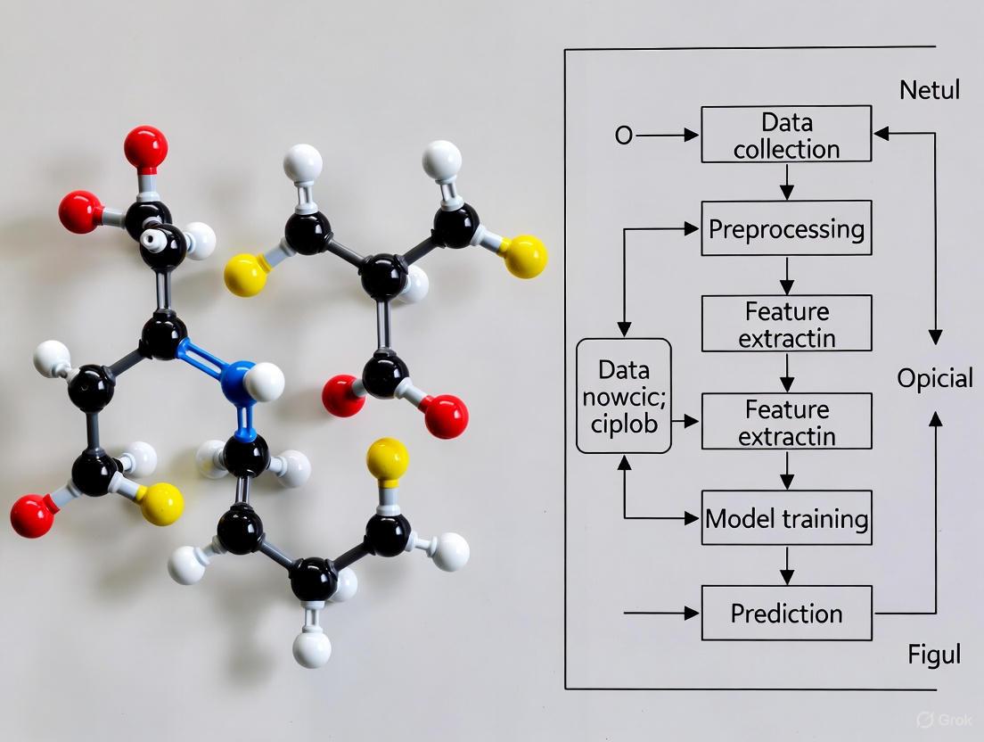
A generalized experimental workflow for smartphone-based environmental analysis research is depicted in the following diagram, illustrating the integration of data collection, machine learning, and outcome application.
Diagram 1: Smartphone Environmental Analysis Workflow.
The Scientist's Toolkit: Research Reagent Solutions
This section details key hardware, software, and data components essential for conducting smartphone-based environmental analysis research.
Table 4: Essential Research Reagents and Materials for Smartphone-Based Environmental Analysis
| Research Reagent / Material | Type | Function in Research |
|---|---|---|
| Low-Cost Air Quality Sensors (PM2.5, CO2) | Hardware | Measures target pollutant concentrations; core component of mobile or static monitoring nodes. |
| Microcontroller (e.g., ESP8266) | Hardware | Interfaces with sensors, manages data collection, and enables wireless data transmission to cloud platforms. |
| Open Data Kit (ODK) | Software | Open-source suite for building mobile data collection forms, used for self-administered smartphone surveys. |
| PurpleAir, AirNow Sensor Networks | Data | Provides extensive, real-time air quality data from public sensor networks for model training and validation. |
| Species Distribution Models (SDMs) | Algorithm | Statistical tools that use species occurrence records and environmental data to estimate geographic ranges and suitable habitats. |
| Community-Sourced Data (e.g., iNaturalist, Biome) | Data | Provides massive volumes of geotagged species observations for training AI models and ecological analysis. |
| Shapley Additive Explanations (SHAP) | Algorithm | An Explainable AI (XAI) method that interprets ML model outputs, quantifying the contribution of each input feature. |
| Gradient Boosting (GB) / k-Nearest Neighbors (kNN) | Algorithm | High-performance ML algorithms used for calibrating low-cost environmental sensors against reference instruments. |
The confluence of smartphone technology and advanced machine learning has created a powerful new paradigm for environmental monitoring. The methodologies and protocols outlined in this guide demonstrate a fundamental shift towards data-driven, hyperlocal, and cost-effective research in air quality, biodiversity, and climate science. The ability to collect and intelligently analyze high-resolution spatiotemporal data is not only filling critical knowledge gaps but also empowering more precise and proactive environmental management and conservation strategies. As these technologies continue to evolve, with advancements in edge computing, 5G, and more sophisticated AI models, their role in understanding and protecting our planetary ecosystems will undoubtedly become even more central to global scientific and policy efforts.
The integration of machine learning (ML) with smartphone-based sensing represents a paradigm shift in environmental monitoring. This synergy enables a transition from centralized, expensive monitoring stations to distributed, real-time data acquisition and analysis. Framed within a broader thesis on the role of machine learning in smartphone-based environmental analysis, this technical guide explores how this convergence creates a powerful value proposition: it facilitates immediate, data-driven decision-making through intelligent alerts while simultaneously empowering a new era of citizen science, democratizing environmental data collection and fostering public engagement in scientific discovery. Advanced machine learning models, including hybrids like MLP-CapSA and resource-efficient networks, are central to transforming raw sensor data into actionable intelligence and credible scientific findings [11] [19].
Technical Foundations of Smartphone-Based Environmental Analysis
The architecture of a smartphone-based environmental monitoring system rests on three core technical pillars: on-device sensors, machine learning models, and data communication protocols.
On-Device Sensing Capabilities
Modern smartphones are equipped with a sophisticated array of sensors capable of measuring a wide range of environmental parameters. These sensors act as the primary data acquisition layer.
- Physical Quantity Sensors: These include sensors for temperature, humidity, atmospheric pressure, light intensity, and sound level, which measure fundamental physical phenomena in the device's immediate surroundings [20].
- Motion and Position Sensors: Accelerometers, gyroscopes, and GPS sensors are instrumental in mobility applications, tracking movement, vibration, and geographic location, which can be correlated with environmental data for spatial analysis [20].
- Chemical Sensing (Emerging): While less common in standard devices, advancements in accessory and integrated sensors are beginning to allow for the detection of certain chemical attributes, such as air quality parameters [20].
Machine Learning Integration and Model Optimization
Machine learning models transform raw sensor readings into meaningful insights. Given the resource constraints of mobile devices, model optimization is critical.
- On-Device ML: Deploying ML models directly on smartphones eliminates cloud dependency, reduces latency by up to 50%, and enhances data privacy. Specialized hardware like Neural Processing Engines enables local inference for tasks like voice recognition and image classification [19].
- Model Optimization Techniques: To ensure performance on mobile hardware, techniques such as quantization (reducing numerical precision of weights) and pruning (removing redundant neurons) are employed. These methods can reduce model size by up to 75% and cut inference times by 30-50% without significant accuracy loss [19].
- Frameworks and APIs: Tools like TensorFlow Lite and PyTorch Mobile are essential for converting and deploying full models into a mobile-optimized format. The Android Neural Networks API (NNAPI) allows for offloading computations to dedicated hardware like GPUs and DSPs, yielding latency reductions exceeding 40% compared to CPU-only processing [19].
Table 1: Key Machine Learning Models for Environmental Analysis on Smartphones
| Model/Algorithm | Primary Application | Key Advantage | Citation |
|---|---|---|---|
| Hybrid MLP-CapSA | Predicting AI education quality (as a proxy for system performance) | High accuracy (R²=0.9803); effective weight optimization | [11] |
| LSTM/GRU Networks | Forecasting energy consumption and indoor air quality (IAQ) | >92% accuracy in time-series prediction of environmental parameters | [21] |
| Pre-trained Models (e.g., MobileNetV3) | Image-based environmental classification (e.g., plant health, pollution) | Fast deployment; high accuracy for real-time inference | [19] |
| Random Forest | Species identification and community structure prediction | High interpretability; handles mixed data types well | [22] [23] |
Experimental Protocols for Validated Research
The credibility of smartphone-based environmental research hinges on rigorous, reproducible experimental methodologies. The following protocols detail two key applications.
Protocol 1: Monitoring Indoor Air Quality (IAQ) and Energy Efficiency
This protocol, adapted from a study balancing IAQ with energy use in buildings, demonstrates the use of ML for multi-objective optimization [21].
1. Objective: To experimentally analyze and optimize HVAC system operation for simultaneous energy savings and maintenance of optimal IAQ using machine learning.
2. Materials and Setup:
- Data Acquisition System: A network of sensors measuring CO₂, particulate matter (PM2.5, PM10), temperature, humidity, and exogenous variables (time, date, rain). Over 35,000 records were collected [21].
- Computational Platform: A system capable of training and deploying recurrent neural network models.
3. Methodology:
- Data Collection: Sensor data is collected in real-time and aggregated into a structured dataset.
- Model Training and Validation: Several ML models, including RNN, LSTM, GRU, and CNN, are trained on the dataset. The models learn to predict future IAQ parameters and energy consumption. Models are validated for robustness using diverse datasets, and their predictions are explained using SHAP (Shapley Additive exPlanations) values [21].
- Implementation: The trained model (with GRU/LSTM achieving >92% accuracy) is deployed to provide real-time control signals to the HVAC system. This enables predictive and pre-emptive adjustments, ensuring energy is not wasted while IAQ remains within healthy thresholds [21].
Diagram 1: IAQ Optimization Workflow
Protocol 2: Citizen Science for Fossil Plant Identification
This protocol outlines a quantitative method for citizen scientists to contribute to paleobotany using machine learning for fossil identification, based on a study of Czekanowskiales [23].
1. Objective: To numerically classify and identify fossil plant genera and species based on morphological trait data using a combination of cluster analysis and supervised learning.
2. Materials:
- Sample Set: A dataset of 80 fossil specimens from 35 species, documented in 206 images from published literature and specimen infrastructures [23].
- Trait Data: Macroscopic (e.g., leaf dimensions, vein density) and cuticular (e.g., stomatal patterns) traits were manually measured and recorded.
3. Methodology:
- Trait Encoding: Qualitative traits (e.g., leaf shape) are converted into numerical values using label encoding or one-hot encoding for ML processing [23].
- Unsupervised Clustering: A hierarchical clustering algorithm is applied to the trait dataset to perform numerical taxonomy and group species without prior labels, validating traditional taxonomic groups [23].
- Supervised Model Training: Five algorithms—Logistic Regression (LR), k-Nearest Neighbors (KNN), Naive Bayes (NB), Classification and Regression Tree (CART), and Support Vector Machine (SVM)—are trained on the labeled trait data. The model learns to map traits to genus and species names [23].
- Identification: The best-performing model (CART and LR in the source study) can be deployed as a mobile-friendly tool. Citizen scientists can input measurements and images of their finds for automated, quantitative identification, overcoming reliance on subjective expert judgment [23].
Table 2: Key Research Reagent Solutions for Environmental and Ecological Analysis
| Item/Reagent | Function/Application | Technical Specification/Note |
|---|---|---|
| IoT Sensor Node | Measures real-time environmental parameters (Temp, Humidity, CO₂, PM) | Integrates with microcontroller (Arduino) and HTTP/Wi-Fi for data transmission [24]. |
| Trait Encoding Scripts | Converts qualitative morphological observations into machine-readable data | Uses Label Encoding or One-Hot Encoding in Python/Pandas for ML readiness [23]. |
| TensorFlow Lite | Framework for deploying pre-trained ML models on mobile and edge devices | Enables real-time inference; supports quantization for model size reduction [19]. |
| SHAP (SHapley Additive exPlanations) | Explains the output of ML models, providing interpretability for predictive outcomes | Critical for validating model decisions in scientific contexts, such as IAQ predictions [21]. |
The Scientist's Toolkit
Implementing the above protocols requires a suite of software and methodological tools.
- iMESc App: An interactive R/Shiny-based application designed to streamline ML workflows for environmental data. It integrates tools for data pre-processing, visualization, and both unsupervised (Self-Organizing Maps, clustering) and supervised (Random Forest, SVM) algorithms, significantly reducing coding time and technical barriers [22].
- Accessible Data Visualization Principles: When presenting findings, ensure visualizations are accessible. This includes using high-contrast colors (≥4.5:1 for text), avoiding color as the sole means of conveying information, providing direct labels and alternative text, and offering data in supplemental formats (e.g., tables) [25].
The value proposition of machine learning in smartphone-based environmental analysis is robust and multi-faceted. It moves beyond simple data logging to enable real-time intelligent alerts for immediate intervention, as demonstrated in IAQ management. Concurrently, it powerfully enables citizen science by providing the public with accessible, quantitative tools for species identification and data collection, thereby expanding the scale and scope of environmental research. The continuous advancement of on-device ML, sensor technology, and user-friendly analytical platforms promises to further deepen this synergy, leading to smarter, more responsive environmental stewardship and a more engaged, scientifically literate public.
From Data to Decisions: ML Algorithms and Workflows for Smartphone Analysis
The proliferation of smartphones has ushered in a new era for environmental analysis research. These ubiquitous devices are equipped with a powerful suite of sensors, including high-resolution cameras, multi-axis inertial measurement units (IMUs), GPS, and microphones, transforming them into versatile, portable data acquisition systems. This capability enables researchers to collect high-frequency, multi-modal data across vast spatial and temporal scales, facilitating a data-driven approach to understanding complex environmental phenomena. Machine learning (ML) forms the computational backbone required to convert this raw, often noisy, sensor data into actionable insights. This whitepaper details a core algorithmic toolkit for smartphone-based research, focusing on three foundational ML architectures: Convolutional Neural Networks (CNNs) for image analysis, Long Short-Term Memory networks (LSTMs) for time-series data, and Random Forest (RF) for classification tasks. The effective application of these algorithms is critical for advancing research in areas such as precision agriculture, environmental monitoring, and human activity recognition.
The Core Algorithms
Convolutional Neural Networks (CNNs) for Image Analysis
CNNs are specialized deep learning architectures designed to process data with a grid-like topology, such as images. Their strength lies in automatically and adaptively learning spatial hierarchies of features from raw pixel data.
Theoretical Foundation: A CNN typically comprises three primary types of layers:
- Convolutional Layers: These layers apply a set of learnable filters (or kernels) to the input image. Each filter slides (convolves) across the input, computing the dot product between the filter weights and the local region of the input, producing a feature map that responds to specific visual patterns like edges, corners, and textures.
- Pooling Layers: These layers perform non-linear down-sampling, reducing the spatial dimensions of the feature maps. This operation decreases the computational load, provides a form of translation invariance, and helps control overfitting. Max pooling is the most common technique, which extracts the maximum value from a set of values.
- Fully-Connected Layers: After several rounds of convolution and pooling, the high-level reasoning is done via fully-connected layers. Every neuron in a fully-connected layer is connected to every neuron in the preceding volume, culminating in a final layer that outputs class probabilities (for classification) or continuous values (for regression).
Application in Smartphone Research: CNNs are predominantly used for tasks involving visual data captured by smartphone cameras.
- Precision Agriculture: A study on citrus leaf disease classification compared MobileNet CNN and a Self-Structured CNN (SSCNN). The SSCNN achieved a validation accuracy of 99%, outperforming MobileNet (92%), and was deemed more suitable for real-time smartphone deployment due to its computational efficiency [26].
- Environmental Monitoring: Research has explored using CNN-based regression models on mobile-captured images to predict air quality indices (AQI) and pollutant concentrations (e.g., PM2.5, NO2). This approach offers a cost-effective alternative to traditional, expensive sensor networks [27].
- Ergonomics and HCI: CNNs like MobileNetV2, Inception V3, and ResNet-50 have been employed to classify smartphone grip postures from images, with an ensemble model achieving an accuracy of 95.9%. This analysis helps in designing more ergonomic user interfaces [28].
Long Short-Term Memory (LSTM) for Time-Series Analysis
LSTM networks are a type of recurrent neural network (RNN) specifically engineered to capture long-range dependencies and temporal patterns in sequential data, a task at which traditional RNNs often fail due to the vanishing gradient problem.
Theoretical Foundation: The key innovation of the LSTM is its memory cell and gating mechanism, which regulates the flow of information. The cell state acts as a conveyor belt, running through the entire sequence chain, with minor linear interactions. This allows information to flow unchanged. The gates are neural networks that selectively add or remove information to the cell state. They are:
- Forget Gate: Decides what information to discard from the cell state.
- Input Gate: Determines which new values from the current input should be updated to the cell state.
- Output Gate: Controls what part of the current cell state is output at the current time step.
Application in Smartphone Research: LSTMs are ideal for analyzing time-series data from smartphone IMUs (accelerometer, gyroscope) and other sequential environmental readings.
- Human Activity Recognition (HAR): LSTM networks excel at classifying human activities (e.g., walking, running, using tools) from smartphone sensor data. A hybrid 4-layer CNN-LSTM model has been shown to enhance recognition performance by automatically learning spatial features and temporal representations, achieving high accuracy on public datasets like UCI-HAR [29]. Enhanced LSTM models incorporating attention and squeeze-and-excitation blocks have demonstrated accuracies of up to 99% on sensor-based HAR tasks [30].
- Advanced Environmental Forecasting: LSTM models, including hybrids with CNNs, are used for complex time-series predictions, such as forecasting PM2.5 and PM10 levels by learning from historical pollution and meteorological data [27].
Random Forest (RF) for Classification
Random Forest is a robust ensemble learning method that operates by constructing a multitude of decision trees at training time. It is renowned for its high accuracy, resistance to overfitting, and ability to handle high-dimensional data.
Theoretical Foundation: Random Forest introduces two key sources of randomness:
- Bagging (Bootstrap Aggregating): Each tree is trained on a random subset of the original training data, drawn with replacement.
- Random Feature Selection: At each split in the decision tree, the algorithm considers only a random subset of features. This de-correlates the individual trees. For classification, the final output is the class selected by the majority of the trees. This collective decision-making process results in a model that is generally more accurate and stable than any single decision tree.
Application in Smartphone Research: RF is widely used for its interpretability and effectiveness in various classification tasks, even with smaller datasets.
- Android Malware Detection: A study on permission-based Android malware detection found that the Random Forest algorithm demonstrated superior performance, achieving an accuracy of 93.96%. The methodology also reduced the feature set size by up to 90% while maintaining this high accuracy, significantly improving the model's running time [31].
- Context-Aware Smartphone Usage Prediction: In predictive modeling of personalized smartphone usage (e.g., predicting call activity), Random Forest is among the suite of classic ML classifiers that have been effectively employed to classify user behavior based on temporal, spatial, and social contexts [32].
- Sensor-Based Hand Gesture Recognition: RF has been used in ensemble models, such as a voting meta-classifier with SVM and Logistic Regression, to classify data glove-captured hand gestures with an accuracy of 95.5% [28].
Quantitative Performance Comparison
The following tables summarize the performance of the discussed algorithms across various smartphone-based research applications.
Table 1: CNN Performance in Smartphone Image-Based Tasks
| Application Domain | Specific Task | CNN Model(s) Used | Reported Performance | Source |
|---|---|---|---|---|
| Precision Agriculture | Citrus Leaf Disease Classification | MobileNet, SSCNN | Training Acc: 98.38% (MobileNet), 98% (SSCNN); Validation Acc: 92% (MobileNet), 99% (SSCNN) | [26] |
| Ergonomics | Smartphone Grip Posture Recognition | Ensemble (MobileNetV2, ResNet-50, Inception V3) | 95.9% Accuracy | [28] |
| Environmental Monitoring | Air Quality (Pollutant) Prediction | Regression-based CNN | Mean Squared Error: 0.0077 (2 pollutants), 0.0112 (5 pollutants) | [27] |
Table 2: LSTM Performance in Smartphone Time-Series Tasks
| Application Domain | Specific Task | LSTM Model(s) Used | Reported Performance | Source |
|---|---|---|---|---|
| Human Activity Recognition | Recognition of Daily/Industrial Activities | LSTM with Attention & SE blocks | 99% Accuracy | [30] |
| Human Activity Recognition | Sensor-based Activity Recognition | 4-layer CNN-LSTM | Accuracy improvement of up to 2.24% over prior approaches | [29] |
| Environmental Forecasting | PM10 Level Prediction | GRU (an LSTM variant) | Best results among RNN, LSTM, and GRU models | [27] |
Table 3: Random Forest Performance in Smartphone Classification Tasks
| Application Domain | Specific Task | Key Features | Reported Performance | Source |
|---|---|---|---|---|
| Cybersecurity | Android Malware Detection | Android Permissions | 93.96% Accuracy | [31] |
| Cybersecurity | Android Malware Detection | Reduced Permission Set (90% less) | 93.96% Accuracy (maintained) | [31] |
| Ergonomics | Hand Gesture Recognition | Voting Classifier (RF, SVM, LR) | 95.5% Accuracy | [28] |
Detailed Experimental Protocols
To ensure reproducibility, this section outlines detailed methodologies for key experiments cited in this whitepaper.
- Data Acquisition: Collect 2,939 images of citrus leaves at the vegetative stage using a smartphone. The dataset should include both healthy and diseased leaves, with diagnoses validated by a plant pathologist.
- Data Preprocessing: Resize all images to a uniform resolution suitable for the chosen CNN input. Augment the dataset using techniques like rotation, flipping, and scaling to increase its size and variability.
- Dataset Splitting: Randomly split the preprocessed image dataset into a training set (e.g., 1787 images) and a validation set.
- Model Training:
- Configure two CNN architectures: MobileNet (version 2) and a Self-Structured CNN (SSCNN).
- Train both models on the same training set, using an appropriate optimizer and loss function (e.g., categorical cross-entropy).
- Monitor the training and validation accuracy and loss over multiple epochs (e.g., 10-12).
- Model Evaluation: Evaluate the final model on the held-out validation set. The primary metric for comparison is validation accuracy. The SSCNN is expected to achieve a higher validation accuracy (~99%) than MobileNet (~92%).
- Data Collection: Use a smartphone's inertial sensors (accelerometer and gyroscope) to collect time-series data while participants perform a predefined set of activities (e.g., walking, sitting, standing, walking upstairs, walking downstairs).
- Data Preprocessing & Segmentation:
- Apply a noise filter to the raw sensor data.
- Segment the continuous data stream into fixed-width sliding windows (e.g., 2.56 seconds). Each window represents one data sample.
- Feature Extraction (for traditional ML) / Model Input Preparation (for LSTM):
- For LSTM: The raw segmented data from the sensors can be fed directly into the network, allowing it to learn features automatically.
- Alternatively, engineered features (e.g., mean, standard deviation) can be calculated for each window.
- Model Training and Validation:
- Design an LSTM-based network architecture. A hybrid CNN-LSTM model (e.g., 4-layer CNN-LSTM) can be used to first extract spatial features with CNN layers before processing the sequence with an LSTM layer.
- Train the model using the segmented data.
- Validate the model using a rigorous protocol such as 10-fold cross-validation or Leave-One-Subject-Out (LOSO) cross-validation to ensure generalizability.
- Performance Measurement: The primary evaluation metric is classification accuracy on the test set, comparing the predicted activities against the ground truth labels.
- Data Collection: Obtain a dataset of Android applications (APKs) containing both benign and malware samples.
- Feature Extraction: Static analysis is performed on each APK to extract the list of requested permissions from the AndroidManifest.xml file. This creates a feature vector for each application where each feature represents a specific Android permission.
- Feature Selection:
- Calculate a feature importance score for each permission (e.g., using Gradient Boosting).
- Rank the permissions based on their importance score and select the top N most important features, significantly reducing the dimensionality of the dataset (e.g., by 90%).
- Model Training:
- Train a Random Forest classifier on the training set, using both the full feature set and the reduced feature set.
- Model Evaluation:
- Evaluate the model on a separate test set. Compare the accuracy, precision, and recall of the model trained on the full feature set versus the reduced set.
- Compare the execution (training) time for both models. The model with the reduced feature set is expected to achieve comparable accuracy with a significantly shorter run-time.
Visualization of Model Architectures and Workflows
CNN-LSTM Hybrid Model for Human Activity Recognition
Random Forest for Android Malware Classification
Essential Research Reagent Solutions
The following table outlines the key "research reagents" — the datasets, software, and hardware — required for conducting smartphone-based ML research.
Table 4: Essential Research Reagents for Smartphone-Based ML Analysis
| Reagent Category | Specific Tool / Resource | Function in Research |
|---|---|---|
| Public Datasets | UCI-HAR Dataset [29] | Benchmark dataset for evaluating Human Activity Recognition models using smartphone sensor data. |
| Public Datasets | PlantVillage Dataset | Large public dataset of plant images, useful for training and validating agricultural disease detection models [26]. |
| Public Datasets | Android Permission-based Datasets [31] | Curated datasets of Android applications with labeled permissions, used for malware detection research. |
| Software Libraries | TensorFlow / Keras, PyTorch | Open-source deep learning frameworks used to build, train, and deploy CNN and LSTM models. |
| Software Libraries | Scikit-learn | Comprehensive machine learning library for implementing Random Forest and other classic ML algorithms, as well as for data preprocessing [31] [32]. |
| Hardware | Modern Smartphone | Primary data acquisition device, providing cameras, IMU sensors (accelerometer, gyroscope), and GPS. Also serves as a deployment platform for real-time models. |
| Computing Resources | GPU-Accelerated Workstation / Cloud Compute | Essential for reducing the time required to train complex deep learning models like CNNs and LSTMs. |
The synergistic application of CNNs, LSTMs, and Random Forest algorithms constitutes a powerful toolkit for advancing smartphone-based environmental analysis. CNNs provide the vision to interpret visual environmental indicators, LSTMs offer the ability to understand temporal patterns in sensor data, and Random Forest delivers robust and efficient classification. As smartphone sensors continue to improve and these machine learning algorithms are further refined and optimized for mobile deployment, their collective impact on research will only grow. This will enable the development of more sophisticated, real-time, and personalized systems for monitoring and responding to complex environmental dynamics, ultimately contributing to smarter and more sustainable interactions with our environment.
The integration of machine learning (ML) with smartphone technology has created a powerful paradigm for environmental analysis research. Smartphones, equipped with a diverse array of embedded sensors and significant processing capabilities, offer an unprecedented platform for collecting high-resolution environmental data and deploying analytical models at scale. This in-depth technical guide details the end-to-end workflow for developing ML systems within the context of smartphone-based environmental analysis, providing researchers and drug development professionals with a structured methodology from initial data collection to final model deployment. The proliferation of smartphones has enabled the creation of extensive datasets, with modern studies leveraging multi-sensor data collection that extends beyond Wi-Fi and Bluetooth to include inertial sensors, magnetometers, and environmental sensors [33]. This guide establishes a foundational framework for leveraging these capabilities in environmental research, with applications ranging from air quality monitoring to ecosystem health assessment.
Data Collection Methodologies
The data collection phase establishes the foundation for any successful ML application in environmental analysis. This process requires careful consideration of sensor selection, data recording protocols, and ethical frameworks.
Smartphone Sensor Capabilities
Modern smartphones contain a sophisticated array of sensors capable of capturing diverse environmental phenomena. The table below summarizes key sensors relevant to environmental analysis research:
Table 1: Smartphone Sensors for Environmental Data Collection
| Sensor Type | Environmental Measurement | Data Format | Research Application |
|---|---|---|---|
| Accelerometer | Vibration patterns, physical disturbances | Triaxial acceleration values (m/s²) | Seismic activity monitoring, infrastructure integrity |
| Magnetometer | Magnetic field strength | Microtesla (μT) | Detection of magnetic pollutants, geological mapping |
| Microphone | Ambient sound levels | Decibels (dB), frequency spectra | Noise pollution studies, biodiversity monitoring via acoustics |
| Ambient Light Sensor | Illuminance | Lux (lx) | Light pollution mapping, forest canopy density analysis |
| Barometer | Atmospheric pressure | Hectopascals (hPa) | Weather pattern prediction, altitude-corrected measurements |
| GPS | Location coordinates | Latitude, longitude | Spatial mapping of environmental parameters |
| Camera | Visual environmental features | RGB image data, video | Land use classification, pollution visualization |
Experimental Protocol for Multi-Modal Data Collection
Comprehensive environmental analysis often requires a multi-modal approach that combines multiple sensing modalities to overcome the limitations of individual sensors [34]. The following protocol ensures consistent, high-quality data collection:
Sensor Calibration: Prior to deployment, calibrate sensors against reference equipment. For example, calibrate smartphone microphones against a reference sound level meter at multiple frequencies (e.g., 250 Hz, 1 kHz, 8 kHz) and barometers against certified pressure standards.
Spatial-Temporal Sampling: Establish systematic sampling strategies that account for both spatial and temporal dimensions. For urban air quality studies, implement a grid-based collection pattern with timed intervals (e.g., samples collected at 100-meter intervals every 2 hours during peak pollution periods).
Multi-Modal Synchronization: Implement hardware-level timestamping with network time protocol (NTP) synchronization to align data streams from different sensors. This enables precise temporal correlation between, for instance, visual observations (camera) and quantitative measurements (other sensors) [34].
Contextual Metadata Recording: Document environmental conditions (temperature, humidity, weather conditions), device information (model, OS version), and collection parameters (orientation, placement) for each sampling event.
Ethical Compliance: Implement privacy-preserving techniques such as data anonymization and secure transmission, particularly when collecting visual or location data in sensitive areas [35]. Obtain necessary institutional review board (IRB) approvals for studies involving human subjects or data from private spaces.
Data Preprocessing Framework
Raw sensor data requires significant preprocessing to become suitable for ML model training. This phase transforms heterogeneous, noisy data streams into clean, structured features.
Preprocessing Pipeline
The preprocessing framework for smartphone-based environmental data consists of several critical stages:
Noise Reduction and Signal Filtering: Apply appropriate digital filters based on signal characteristics. For inertial sensor data, use a high-pass filter (cutoff frequency 0.1-0.5 Hz) to remove gravitational components, followed by a low-pass filter (cutoff frequency 15-20 Hz) to reduce high-frequency noise [35]. For audio environmental data, implement band-pass filtering to focus on relevant frequency ranges.
Data Imputation and Gap Filling: Address missing data points using sophisticated imputation methods. For short gaps (<5 seconds) in environmental time series, employ linear interpolation. For longer gaps, use sensor fusion techniques to estimate missing values from correlated sensors [34].
Temporal Alignment: Synchronize heterogeneous data streams using dynamic time warping algorithms or cross-correlation techniques to address differing sampling rates across sensors [34].
Feature Extraction: Derive informative features from raw sensor data. For environmental analysis, particularly relevant features include:
- Statistical Features: Mean, standard deviation, median, percentiles (25th, 75th)
- Spectral Features: Fast Fourier Transform (FFT) coefficients, spectral entropy, dominant frequencies
- Temporal Features: Autocorrelation coefficients, trend analysis, seasonal decomposition
- Cross-Sensor Features: Correlation coefficients between different sensor modalities
The following diagram illustrates the complete preprocessing workflow:
Data Quality Validation
Implement automated quality validation checks throughout the preprocessing pipeline:
- Sensor Integrity Verification: Detect sensor malfunctions through range checks (e.g., magnetometer readings outside Earth's typical 25-65 μT field) and consistency checks across redundant sensors.
- Signal Quality Indicators: Compute signal-to-noise ratios for each data segment and flag low-quality recordings for manual review or exclusion.
- Statistical Process Control: Establish control charts for key parameters to detect systematic deviations from expected distributions.
Model Training and Algorithm Selection
The model training phase transforms preprocessed sensor data into predictive capabilities for environmental analysis.
Machine Learning Approaches for Environmental Analysis
Different environmental monitoring tasks require specialized algorithmic approaches:
Table 2: ML Algorithms for Smartphone Environmental Analysis
| Algorithm Category | Specific Algorithms | Environmental Applications | Performance Considerations |
|---|---|---|---|
| Traditional ML | Random Forest, SVM, XGBoost | Air/water quality classification, pollution source identification | AUC: 95-98%, Accuracy: 85-92% [35] |
| Deep Learning | CNN, LSTM, Transformer Networks | Complex pattern recognition in multi-modal sensor data, temporal forecasting | Improved accuracy but higher computational cost [33] |
| Hybrid Approaches | CNN-LSTM, MLP with nature-inspired optimizers | Predictive modeling of environmental trends, quality assessment | CCC: 0.96, R²: 0.98 [11] |
| Lightweight Models | Pruned Neural Networks, MobileNet | Real-time on-device environmental monitoring | 30-50% reduction in model size with <5% accuracy drop [35] |
Experimental Protocol for Model Development
A rigorous methodology ensures robust model performance across diverse environmental conditions:
Data Partitioning: Implement stratified splitting to maintain distribution of important environmental variables (e.g., seasonal variations, geographic diversity). Recommended split: 70% training, 15% validation, 15% testing.
Cross-Validation Strategy: Use grouped k-fold cross-validation (k=5) where data from the same location or time period are kept together within folds to prevent leakage and ensure generalizability.
Hyperparameter Optimization: Employ Bayesian optimization or genetic algorithms like Capuchin Search Algorithm (CapSA) for efficient hyperparameter tuning, which has demonstrated superior performance in environmental prediction tasks [11].
Model Training with Regularization: Implement early stopping with a patience of 10-20 epochs and apply appropriate regularization techniques (L1/L2, dropout) to prevent overfitting, particularly important with limited environmental datasets.
Ensemble Methods: Combine predictions from multiple models (e.g., Random Forest, Gradient Boosting, and Neural Networks) through stacking or averaging to improve robustness and accuracy.
The following diagram illustrates the model architecture selection and training workflow:
Performance Metrics for Environmental Models
Evaluation of environmental ML models requires comprehensive assessment across multiple dimensions:
- Predictive Accuracy: Standard classification metrics (accuracy, precision, recall, F1-score) and regression metrics (RMSE, MAE, R²) specific to environmental applications.
- Temporal Stability: Model performance consistency across different time periods and seasonal variations.
- Spatial Generalizability: Performance transferability across different geographic areas and environmental conditions.
- Computational Efficiency: Inference latency, memory footprint, and power consumption - critical factors for smartphone deployment.
Model Deployment and Implementation
The deployment phase transitions trained models from research environments to operational smartphone-based environmental monitoring systems.
Deployment Architecture Options
Selecting an appropriate deployment architecture involves critical trade-offs between capability, latency, and resource consumption:
Table 3: Deployment Architectures for Environmental ML Models
| Architecture | Implementation | Advantages | Limitations | Environmental Use Cases |
|---|---|---|---|---|
| Cloud-Based | Model hosted on server, smartphones send data via APIs | Handles complex models, continuous learning, easy updates | Network dependency, latency, data transmission costs | Large-scale environmental modeling, historical analysis |
| On-Device | Model deployed directly on smartphone (TFLite, Core ML) | Works offline, low latency, enhanced privacy, reduced server costs | Limited to simpler models, storage constraints, update challenges | Real-time pollution alerts, wildlife sound classification |
| Hybrid | Split processing between device and cloud | Balances performance and capability, adaptive functionality | Implementation complexity, testing overhead | Multi-modal environmental sensing with both real-time and historical analysis [36] |
Implementation Protocol for Mobile Deployment
A structured deployment methodology ensures reliable performance in real-world environmental monitoring scenarios:
Model Optimization: Convert models to efficient formats (TensorFlow Lite, PyTorch Mobile) using techniques such as quantization (FP16 or INT8), pruning, and layer fusion to reduce size by 40-60% with minimal accuracy loss [36].
Edge Computing Integration: Leverage smartphone hardware acceleration (GPUs, NPUs) for efficient model inference. Implement adaptive sampling rates that balance battery consumption with data quality requirements.
Continuous Monitoring and Model Updating: Deploy MLflow or similar MLOps platforms to track model performance metrics in production [37]. Implement mechanisms for federated learning to update models across devices without centralizing raw environmental data.
Resource Management: Develop intelligent scheduling algorithms that coordinate sensor usage, data processing, and transmission to minimize battery consumption while maintaining monitoring objectives.
The following diagram illustrates the complete end-to-end workflow integrating all phases:
The Scientist's Toolkit: Research Reagent Solutions
This section details essential computational tools and frameworks for implementing smartphone-based environmental ML systems.
Table 4: Essential Research Tools for Smartphone Environmental ML
| Tool Category | Specific Solutions | Function in Research Workflow | Environmental Analysis Applications |
|---|---|---|---|
| ML Frameworks | TensorFlow, PyTorch, Scikit-learn | Model development, training, and evaluation | Flexible model architectures for diverse environmental data types [37] |
| Mobile ML Libraries | TensorFlow Lite, Core ML, ML Kit | Model optimization and on-device deployment | Efficient inference for real-time environmental monitoring [36] |
| Data Processing | Pandas, NumPy, SciPy | Data cleaning, transformation, and feature engineering | Processing of temporal environmental sensor data streams |
| Visualization | TensorBoard, Matplotlib, Seaborn | Model interpretation and result communication | Visualization of environmental patterns and model performance |
| Workflow Management | MLflow, Kubeflow | Experiment tracking, model versioning, and deployment | Reproducible environmental monitoring pipelines [37] |
| Sensor Integration | Android Sensor API, iOS Core Motion | Raw data acquisition from smartphone sensors | Unified access to accelerometer, magnetometer, and environmental sensors |
This technical guide has presented a comprehensive framework for implementing end-to-end ML workflows within smartphone-based environmental analysis research. By methodically addressing each phase from multi-modal data collection through optimized model deployment, researchers can develop robust systems capable of monitoring and analyzing environmental phenomena at unprecedented scales. The integration of sophisticated ML algorithms with ubiquitous smartphone technology creates powerful opportunities for advancing environmental science, enabling real-time monitoring, predictive modeling, and ultimately contributing to more effective environmental conservation and public health interventions. As the field evolves, emerging approaches such as federated learning for privacy-preserving model improvement and advanced neural architectures for multi-modal data fusion will further enhance the capabilities of these systems, opening new frontiers in environmental intelligence.
The integration of artificial intelligence (AI) with smartphone-based imaging has revolutionized ecological monitoring, enabling scalable biodiversity data collection. This technological synergy addresses a critical challenge in conservation biology: the need for extensive, high-quality species occurrence data to inform policy and track global biodiversity targets, such as the Kunming-Montreal Global Biodiversity Framework's "30 by 30" initiative [17]. Smartphones act as ubiquitous sensors, equipped with high-resolution cameras, GPS, and processing power, while machine learning models provide the intelligence for accurate species identification. This combination has transformed millions of citizens into potential data contributors, dramatically accelerating the pace and scale of ecological data acquisition. Community-sourced data, once viewed with skepticism, is now demonstrating significant scientific value, improving the accuracy of Species Distribution Models (SDMs) and providing a critical tool for researchers and policymakers [17]. This guide examines the technical foundations, methodologies, and performance of these AI-driven identification systems, providing a comprehensive resource for researchers implementing these technologies in environmental analysis.
Core AI Technologies and Architectures
The engine behind modern species identification is deep learning, specifically convolutional neural networks (CNNs) and transformer-based models designed for computer vision tasks. These architectures learn hierarchical feature representations directly from pixel data, enabling them to distinguish subtle morphological differences between species.
Predominant Model Architectures
- ResNet (Residual Networks): A cornerstone architecture in many ecological applications, ResNet's residual connections enable the training of very deep networks by mitigating the vanishing gradient problem. ResNet-18 and ResNet-50 are frequently deployed in camera trap imagery analysis, such as in the MLWIC2 project and the North America Camera Trap Images (NACTI) dataset classification [38]. Their efficiency and performance make them suitable for both cloud and edge computation.
- ResNeXt: An extension of ResNet, ResNeXt employs a grouped convolution strategy that increases model capacity without exponentially growing computational complexity. It has demonstrated superior performance as a base model in ensemble learning methods, achieving recalls exceeding 98% for common species in camera trap data [39].
- Vision Transformers (ViT): Leveraging self-attention mechanisms, ViT models treat images as sequences of patches, capturing global contextual information effectively. They are increasingly used as base models in ensemble systems, competing with traditional CNNs [39].
- Ensemble Learning: To maximize accuracy, many production systems combine predictions from multiple base models (e.g., ResNet-18, ResNeXt-50, ViT-Base). This approach improves both precision and recall by mitigating individual model weaknesses and leveraging collective intelligence [39].
Specialized Algorithms for Ecological Challenges
Real-world ecological data presents unique challenges like severe class imbalance (long-tailed distributions) and the need to leverage contextual metadata.
- Long-Tail Recognition (LTR) Strategies: In datasets like NACTI, where a few species (e.g., domestic cow) dominate the samples, standard models fail on rare classes. Advanced solutions include:
- LTR-Specific Loss Functions: Focal Loss [38], Weighted Cross-Entropy [38], and Label-Distribution-Aware Margin (LDAM) loss [38] adjust the learning objective to focus on harder or rarer examples.
- Decoupled Learning: This strategy separates feature learning from classifier training, using instance-balanced sampling for robust features and class-balanced sampling for the classifier [38].
- Regularization Tuning: Careful tuning of weight decay parameters prevents classifier bias toward dominant classes, a method shown to outperform many sophisticated LTR approaches [38].
- Metadata Integration: Boosting identification accuracy involves fusing image data with field occurrence records. A study on Japanese odonates demonstrated that combining image recognition with geographical distribution data increased Top-1 accuracy from 54.6% to 66.8%, as the system could eliminate improbable species suggestions based on known location data [40].
Experimental Protocols and Methodologies
Implementing a robust species identification system requires a methodical approach from data acquisition to model deployment. The following workflow outlines the standard protocol.
Data Acquisition and Curation Strategies
The foundation of any effective model is a diverse, well-curated dataset. Multiple sourcing strategies are employed to build comprehensive image corpora.
- Citizen Science Platforms: Mobile apps like Biome [17], iNaturalist [41], and Pl@ntNet [41] gamify data collection, rapidly amassing millions of geotagged observations. For instance, the Biome app accumulated over 6.5 million observations in Japan within four years [17].
- Camera Traps: Motion-activated cameras (e.g., in the Snapshot Serengeti [39] and NACTI [38] projects) generate vast volumes of "in-the-wild" imagery. The NACTI dataset contains 3.7 million images from 48 animal species across five U.S. sites [38].
- Web Scraping and Digitization: Images are systematically collected from open-access websites and digitized from scientific literature and museum specimens. A study on Odonates created a dataset of 4,571 web-scraped and 4,005 scanned images for 204 species [40].
Data Preprocessing and Annotation
Raw images require significant preprocessing to be suitable for model training.
- Image Augmentation: Techniques like random affine transformation, rotation, flip-flop, and noise addition are applied to increase dataset size and variability, improving model generalization [40]. This is critical for species with few available images.
- Automated Mask Generation for Segmentation: For pixel-level segmentation (e.g., mapping tree species in UAV imagery), weakly labeled citizen science photos can be transformed using foundation models. One workflow uses Grad-CAM to identify salient regions in a classified image, which then guides the Segment Anything Model (SAM) to generate precise segmentation masks automatically, eliminating the need for manual pixel-wise annotation [41].
- Background Replacement: To improve model transferability from close-range citizen science photos to aerial drone imagery, the original background of segmented subjects can be replaced with common background samples from drone imagery [41].
Model Training and Evaluation
The training phase must account for the inherent challenges of ecological data.
- Handling Class Imbalance: Instead of naive random sampling, use class-balanced sampling or deferred re-weighting (DRW) schedules [38]. LDAM loss combined with a DRW scheduler has shown particularly strong performance on long-tailed datasets like NACTI [38].
- Evaluation Metrics: Beyond overall accuracy, a comprehensive evaluation uses a suite of metrics:
- Top-1 and Top-5 Accuracy: Standard for classification tasks.
- Class-wise Recall and Precision: Essential for diagnosing performance on rare "tail" classes.
- F1-Score: Harmonic mean of precision and recall.
- CCC, SROCC, PLCC: Used in specialized studies for assessing correlation and agreement [11].
- Cross-Dataset Validation: To test model robustness, performance should be evaluated on a separate, out-of-distribution dataset. For example, a model trained on NACTI can be validated on the ENA-Detection dataset to simulate domain shift [38].
Performance Data and Comparative Analysis
Quantitative performance varies based on taxonomic group, data quality, and model architecture. The following tables synthesize key metrics from recent studies.
Table 1: Performance Metrics of Species Identification Models Across Studies
| Study / Model | Taxonomic Group / Dataset | Key Metric | Reported Performance | Notable Conditions |
|---|---|---|---|---|
| SpeciesNet (Wildlife Insights) [42] | General Wildlife (Camera Traps) | Detection Recall | 99.4% | Identifies animal presence in images |
| Detection Precision | 98.7% | When model predicts animal is present | ||
| Species-level Accuracy | 94.5% | When making a species-level prediction | ||
| Ensemble Model (ResNeXt-50 base) [39] | Common Camera Trap Species | Recall (In-sample) | >98% (most species) | On Snapshot Serengeti dataset |
| Precision (In-sample) | >97% (most species) | Except for Gazelle Grants | ||
| Automation Rate | 80.67% | |||
| LTR-Optimized Model [38] | NACTI (48 species) | Top-1 Accuracy | 99.40% | With LDAM loss & LTR scheduling |
| Biome App Community ID [17] | Birds, Reptiles, Mammals, Amphibians | Identification Accuracy | >95% | By citizen scientists using the app |
| Seed Plants, Molluscs, Fishes | Identification Accuracy | <90% | ||
| Image + Distribution Data [40] | Japanese Odonates (204 species) | Top-1 Accuracy | 66.8% | Combined images & occurrence records |
| Top-3 Accuracy | 87.3% | Combined images & occurrence records |
Table 2: Impact of Data Blending on Model Performance for Endangered Species [17]
| Data Source | Records Required for Accurate SDM (Boyce index ≥ 0.9) | Model Accuracy (Example) | Spatial Coverage Bias |
|---|---|---|---|
| Traditional Survey Data Only | >2000 records | Lower baseline | Biased towards natural, remote areas |
| Blended Data (Traditional + Community-Sourced) | ~300 records | Significantly Improved | Uniform coverage across urban-natural gradients |
The Scientist's Toolkit: Essential Research Reagents and Platforms
Implementing a smartphone-based species identification system requires a suite of software, hardware, and data resources.
Table 3: Essential Research Reagents and Platforms for AI-Driven Species Identification
| Tool / Platform Name | Type | Primary Function | Key Features / Applications |
|---|---|---|---|
| Wildlife Insights / SpeciesNet [42] [43] | AI Model & Platform | Wildlife identification from camera trap images | Open-source; trained on >65M images; supports ~2,000 species categories |
| Biome [17] | Mobile Application | Citizen science data collection & species ID | Gamification elements; >6M observations in Japan; high user engagement |
| iNaturalist / Pl@ntNet [41] | Mobile Application & Platform | Citizen science data collection & species ID | Research-grade data; community validation; integration with GBIF |
| Segment Anything Model (SAM) [41] | Foundation Model | Generic object segmentation | Generates pixel-level masks from prompts; used in automated mask generation |
| Grad-CAM [41] | Algorithm | Visual explanation of CNN decisions | Highlights discriminative image regions; guides SAM for mask generation |
| TensorFlow / PyTorch [44] | Framework | Model development & training | Core ML frameworks for building and training custom CNN models |
| OpenCV [44] | Library | Computer vision pre-processing | Real-time image processing, transformation, and feature extraction |
| Global Biodiversity Information Facility (GBIF) [41] [17] | Data Repository | Aggregated species occurrence data | Source of historical and citizen science distribution records |
Image-based species identification powered by smartphone cameras and AI has matured into a scientifically robust tool that is reshaping ecological monitoring. The synthesis of community-sourced data, advanced deep learning architectures, and thoughtful ecological modeling has demonstrated tangible benefits, including improved species distribution models and more efficient conservation planning [17]. The key to success lies in addressing the fundamental challenges of data quality, class imbalance, and model generalizability.
Future developments will likely focus on several frontiers. On-device AI will enable real-time identification without network connectivity, further democratizing use in remote field settings. The integration of multimodal data (e.g., sound, environmental DNA, hyperspectral imaging from smartphone cameras [45]) will provide richer contextual information for identification. Advances in explainable AI (XAI) will build greater trust in model predictions among conservation professionals and the public. Finally, the development of even more sophisticated LTR techniques will be crucial for protecting the rarest and most endangered species, which are often the most critical conservation targets. As these technologies continue to converge, they will form an increasingly vital infrastructure for global biodiversity assessment and protection, empowering a new era of data-driven environmental stewardship.
The proliferation of smartphone technology and environmental sensors has created unprecedented opportunities for hyperlocal environmental analysis. This technical guide examines the convergence of sensor fusion and machine learning (ML) to predict local air quality, framing this methodology within a broader research thesis on smartphone-based environmental analysis. Traditional air quality monitoring relies on sparse, regulatory-grade stations which, while accurate, lack the spatial resolution for community-level assessment [46]. The integration of multi-sensor data fusion with advanced ML algorithms enables researchers to overcome these limitations, creating dense, real-time pollution mapping networks that transform smartphones into powerful environmental sensing platforms [47] [46].
Sensor fusion addresses critical gaps in environmental monitoring by integrating heterogeneous data streams from fixed sensors, mobile devices, satellite imagery, and meteorological stations [47] [46]. This multi-layered approach provides the comprehensive data foundation required for ML models to accurately characterize complex pollution dynamics across urban landscapes. For researchers and pharmaceutical professionals, these advancements offer new pathways for investigating exposure-related health impacts and developing targeted interventions based on high-resolution environmental data [46].
Sensor Fusion Fundamentals for Air Quality Monitoring
Multi-Sensor Data Fusion Architectures
Sensor fusion systematically integrates data from multiple sensors to achieve more reliable, accurate, and comprehensive environmental information than can be obtained from individual sensors alone [48]. In air quality monitoring, this involves combining data from physical pollutant sensors, smartphone-embedded sensors, satellite observations, and meteorological stations. The fusion process occurs at different processing levels, each with distinct characteristics and applications [47]:
Table: Levels of Data Fusion in Air Quality Monitoring
| Fusion Level | Processing Stage | Description | Application in Air Quality |
|---|---|---|---|
| Signal Level | Raw signal | Combines raw signals from different sensors to create a new signal with better signal-to-noise ratio | Fusing raw electrical signals from multiple low-cost PM2.5 sensors |
| Pixel Level | Pixel-by-pixel | Generates a fused image where information for each pixel is determined from corresponding pixels in source images | Merging satellite imagery with different spatial resolutions |
| Feature Level | Feature extraction | Extracts and combines salient features (edges, textures, patterns) from various data sources | Combining pollution features from fixed and mobile sensor networks |
| Decision Level | High-level inference | Merges interpretations from multiple algorithms or sensors to yield a final fused decision | Combining classifications from different ML models for final AQI assessment |
Effective air quality prediction systems leverage diverse sensor technologies, each contributing unique capabilities to the fused solution:
- Low-cost IoT Sensors: Measures particulate matter (PM2.5, PM10), nitrogen dioxide (NO₂), ozone (O₃), carbon monoxide (CO), and sulfur dioxide (SO₂) at ground level [49] [50]. These form the dense network backbone for hyperlocal monitoring.
- Satellite Remote Sensors: Provide broad spatial coverage of aerosol optical depth and atmospheric composition [47]. Platforms like Landsat and Sentinel offer critical regional context.
- Smartphone-Embedded Sensors: Modern smartphones contain multiple relevant sensors including cameras (for visual assessment), barometers (pressure), thermometers (temperature), and hygrometers (humidity) that can provide contextual environmental data [51].
- Meteorological Stations: Deliver complementary data on wind speed/direction, temperature, humidity, and precipitation that significantly influence pollutant dispersion and transformation [46].
The fusion of these heterogeneous data sources creates a comprehensive environmental picture that enables more accurate pollution forecasting and source attribution than any single data source can provide.
Machine Learning Framework for Sensor Fusion
Algorithm Selection and Architecture
Machine learning transforms multi-sensor data into actionable predictions through specialized algorithms tailored to handle the temporal, spatial, and multivariate nature of air quality data. Research demonstrates distinct performance characteristics across algorithm categories [49] [46]:
- Ensemble Methods: Random Forest and Extreme Gradient Boosting (XGBoost) consistently achieve high accuracy with structured datasets, effectively handling non-linear relationships between pollution drivers and concentrations [49] [46]. These algorithms excel at feature importance analysis, identifying which sensors and variables most significantly impact prediction accuracy.
- Deep Learning Architectures: Long Short-Term Memory (LSTM) networks capture temporal dependencies in pollution trends, while Convolutional Neural Networks (CNNs) identify spatial patterns across sensor networks [49] [46]. Hybrid models (CNN-LSTM) simultaneously model spatio-temporal relationships for superior forecasting capability.
- Unsupervised Approaches: Clustering algorithms (K-means, DBSCAN) identify pollution hotspots and characterize typical pollution patterns, while anomaly detection methods flag sensor malfunctions or unusual pollution events [49].
The diagram below illustrates the typical ML workflow for sensor fusion-based air quality prediction:
Advanced Fusion Techniques
Modern sensor fusion systems employ sophisticated algorithms to overcome data heterogeneity and quality challenges:
- Kalman Filtering: Recursively estimates pollutant concentrations by integrating noisy sensor measurements with predictive models, continuously refining estimates as new data arrives [48]. Particularly effective for real-time sensor data streams with varying precision.
- Bayesian Inference: Provides probabilistic reasoning framework that incorporates prior knowledge about pollution patterns and updates beliefs based on observed sensor evidence [48]. Handles uncertainty explicitly, crucial when dealing with low-cost sensor data.
- Wavelet Analysis: Decomposes signals into different frequency components, enabling effective feature extraction and denoising of sensor data [47]. Useful for separating true pollution signals from high-frequency noise in urban environments.
- Consensus Filtering: Iteratively refines estimates by reaching consensus among multiple sensors, depreciating outlying values while weighting consistent measurements higher [48]. Enhances system reliability when individual sensors may malfunction.
Experimental Protocols and Methodologies
Sensor Deployment and Data Collection Protocol
Implementing a robust sensor fusion system requires meticulous experimental design. The following protocol ensures high-quality, research-grade data:
Network Design: Deploy fixed sensors at strategic locations representing diverse microenvironments (traffic intersections, parks, industrial boundaries, residential areas). Spatial distribution should follow population density patterns and account for known pollution sources [46].
Mobile Sensor Integration: Equip public transit vehicles or dedicated mobile platforms with calibrated sensors to capture spatial gradients. Mobile routes should be designed to intersect with fixed sensor locations for continuous calibration [46].
Temporal Synchronization: Implement Network Time Protocol (NTP) across all sensors to ensure precise temporal alignment. Data collection should occur at minimum 5-minute intervals to capture diurnal pollution patterns [46].
Reference Calibration: Co-locate a subset of low-cost sensors with regulatory-grade monitoring equipment for drift correction and calibration transfer. Perform weekly zero/span checks to maintain data quality [49].
Meteorological Data Integration: Interface with local weather stations or deploy supplementary sensors to capture wind speed/direction, temperature, humidity, and precipitation at comparable temporal resolution [46].
Data Preprocessing and Quality Control Pipeline
Raw multi-sensor data requires extensive preprocessing before fusion and analysis:
- Missing Data Imputation: Apply multivariate imputation by chained equations (MICE) using correlations across sensors and environmental variables to estimate missing values [46].
- Outlier Detection: Implement isolation forests or DBSCAN clustering to identify and flag sensor malfunctions or physiologically impossible measurements [49].
- Spatio-Temporal Alignment: Resample all data streams to common temporal resolution (e.g., 1-hour intervals) and spatial grid (e.g., 100m × 100m cells) using interpolation techniques appropriate for each data type [47].
- Cross-Sensor Calibration: Apply Bayesian linear regression to align measurements from different sensor types and manufacturers, using co-located measurements as reference [49].
Table: Essential Research Reagents and Computational Tools
| Category | Item | Specification/Function | Research Purpose |
|---|---|---|---|
| Sensing Hardware | PM2.5/PM10 Sensors | Laser scattering detection (e.g., Plantower PMS5003) | Particulate matter quantification at μg/m³ resolution |
| Multi-gas Sensors | Metal oxide semiconductor (MOS) or electrochemical | Detection of NO₂, O₃, CO, SO₂ concentrations | |
| Reference Monitors | Federal Equivalent Method (FEM) certified instruments | Low-cost sensor calibration and validation | |
| Meteorological Station | Wind speed/direction, temperature, humidity, pressure | Contextual atmospheric condition monitoring | |
| Computational Framework | ML Libraries | Scikit-learn, XGBoost, TensorFlow/PyTorch | Model development and training |
| Spatio-temporal Analysis | PostgreSQL with PostGIS, GeoPandas | Spatial data management and processing | |
| Signal Processing | Kalman filters, wavelet transforms, Fourier analysis | Sensor data denoising and fusion | |
| Data Sources | Satellite Data | MODIS, Sentinel-5P TROPOMI | Regional aerosol and pollutant column density |
| Traffic Data | Municipal traffic counters, TomTom, Google Maps | Anthropogenic emission source characterization | |
| Demographic Data | Census data, land use records | Vulnerability and exposure assessment |
Model Training and Validation Methodology
Robust model development follows a structured experimental protocol:
Data Partitioning: Temporally split data into training (70%), validation (15%), and test (15%) sets, maintaining temporal order to prevent data leakage. The test set should represent the most recent time period [46].
Feature Engineering: Create lagged variables (1-24 hour pollution levels), temporal features (hour-of-day, day-of-week, season), spatial features (distance to roads, elevation, land use), and meteorological interactions (temperature × humidity) [46].
Model Training: Implement nested cross-validation with outer temporal folds for performance estimation and inner folds for hyperparameter tuning. This approach provides unbiased performance estimates for time-series data [49].
Interpretability Analysis: Apply SHapley Additive exPlanations (SHAP) to quantify feature importance and visualize relationships between input variables and predictions. This transparency is critical for stakeholder trust and scientific validation [46].
The following diagram illustrates the complete experimental workflow from sensor deployment to model interpretation:
Implementation Challenges and Research Directions
Technical and Practical Implementation Barriers
Despite promising results, operational sensor fusion systems face significant challenges:
- Data Heterogeneity: Integrating sensors with different formats, accuracy, precision, and sampling rates requires sophisticated normalization and alignment techniques [48]. This heterogeneity complicates real-time processing and model deployment.
- Computational Complexity: Fusion algorithms, particularly deep learning models, demand substantial processing resources, creating barriers for real-time applications on resource-constrained devices [49] [48].
- Generalizability Limitations: Models trained in specific urban environments often perform poorly when transferred to new locations with different pollution sources, meteorology, or topography [49].
- Explainability Deficits: The "black box" nature of complex ML models hinders stakeholder trust and regulatory acceptance, despite techniques like SHAP providing partial mitigation [49] [46].
Emerging Research Frontiers
Active research areas address these challenges while expanding analytical capabilities:
- Cross-domain Fusion: Integrating unconventional data sources including social media activity, traffic camera feeds, and municipal infrastructure sensors to create more holistic environmental understanding [48].
- Edge Computing: Deploying lightweight ML models directly on sensor hardware or smartphones to reduce latency and bandwidth requirements while preserving privacy [51].
- Transfer Learning: Developing domain adaptation techniques that enable models trained in data-rich environments to function effectively in locations with sparse monitoring infrastructure [49].
- Federated Learning: Training models across decentralized devices without exchanging raw data, addressing privacy concerns while leveraging diverse observational data [51].
For pharmaceutical and public health researchers, these advancements enable unprecedented granularity in exposure assessment, clinical trial site selection, and investigation of pollution-health outcome relationships. The integration of real-time pollution predictions with health records opens new avenues for understanding acute exposure impacts and developing targeted interventions for vulnerable populations [46].
Sensor fusion coupled with machine learning represents a paradigm shift in local air quality prediction, transforming smartphones from communication devices into distributed environmental sensing platforms. The technical framework outlined in this guide provides researchers with a comprehensive methodology for developing robust prediction systems that overcome limitations of traditional monitoring approaches. As these technologies mature, they offer pharmaceutical and public health professionals powerful tools for exposure assessment and health intervention planning. The continuing evolution of sensor technologies, fusion algorithms, and machine learning techniques promises even greater capabilities for understanding and mitigating the health impacts of air pollution in urban environments.
Navigating the Challenges: Data, Performance, and Computational Efficiency
The integration of citizen-generated data from smartphones and other personal devices is revolutionizing environmental analysis research. This approach enables the collection of high-resolution, spatiotemporal data at a scale previously unattainable through traditional monitoring networks [52] [14]. Machine Learning (ML) stands as the critical engine that transforms these raw, often messy, citizen-generated inputs into robust, scientifically valid data. However, the path from raw collection to research-ready dataset is fraught with significant challenges related to data quality, sheer volume, and systematic biases. This technical guide details these hurdles within the context of smartphone-based environmental research and provides a structured framework, supported by ML-driven methodologies, to overcome them.
The Triad of Challenges in Citizen-Generated Data
The value of citizen-generated data is immense, but its effective utilization requires a clear understanding of its inherent limitations. These challenges can be categorized into three primary areas, which ML strategies are uniquely positioned to address.
- Data Quality and Veracity: Sensor data from consumer-grade smartphones can suffer from calibration errors, unknown measurement contexts (e.g., a user taking a pressure reading on a high floor of a building), and sensor heterogeneity across different device manufacturers [52] [53].
- Data Volume and Velocity: The continuous operation of smartphone sensors can generate massive data streams. The Four V's of Big Data—Volume, Variety, Velocity, and Veracity—are fully present, requiring robust computational infrastructure and efficient algorithms for processing and analysis [54].
- Spatial and Behavioral Bias: Data collection is rarely uniform. It is often concentrated in urban areas and along transportation corridors, leading to spatial gaps. Furthermore, the behavior of citizen observers—categorized broadly as "explorers" who seek new areas and "followers" who cluster around known points—introduces significant non-random sampling biases that can skew environmental models if left uncorrected [55] [14].
Machine Learning Solutions for Data Quality and Standardization
Before citizen-generated data can be used for analysis, it must undergo rigorous quality control and standardization. Machine learning models are particularly effective in automating and scaling these processes.
Quality Control and Bias Correction Protocols
Example: Bias Correction for Smartphone Pressure Data A study utilizing labeled smartphone pressure data from a weather app demonstrated a protocol for correcting sensor biases using a Random Forest machine learning model [52].
- Objective: To correct systematic errors in smartphone-derived atmospheric pressure measurements and apply the corrected data to evaluate the intensity of landfalling tropical cyclones.
- Data Preprocessing: The initial quality control involved three steps:
- Removing pressure values outside a physically plausible range (e.g., 300–1100 hPa).
- Filtering out data points with unrealistic altitude values derived from pressure.
- Correcting pressure readings to sea level using temperature and altitude data.
- Machine Learning Correction: A Random Forest model was trained to predict the bias between each labeled smartphone's pressure reading and a reference value from a professional weather station. The model used features such as the smartphone's recorded pressure, temperature, relative humidity, GPS coordinates, and the device's internal temperature.
- Outcome: This method significantly outperformed models using unlabeled data, reducing the Mean Absolute Error (MAE) from 3.105 hPa to 0.904 hPa. The corrected data revealed that the official best-track dataset consistently underestimated the minimum sea-level pressure of tropical cyclones by a median of 0.51 hPa [52].
Example: Addressing Spatial Bias in Species Distribution Models In ecological studies, citizen science data is often biased by uneven observer behavior. A novel approach was developed to correct for this using a behavioral paradigm [55].
- Objective: To improve the accuracy of Species Distribution Models (SDMs) by correcting for spatial bias introduced by varying observer behaviors ("explorers" vs. "followers").
- Methodology: The researchers used a bias incorporation approach within the SDM framework:
- A bias proxy covariate was created using a k-Nearest Neighbors (k-NN) algorithm to quantify the sampling density around each observation.
- This covariate was included in the species distribution model during training.
- During prediction, the bias covariate was set to a constant value to effectively correct for the uneven sampling effort.
- Outcome: The study found that the optimal strength of the correction (e.g., the number of neighbors 'k' in k-NN) depended on the ratio of explorers to followers in the observer cohort. This data-driven, behaviorally-aware correction method led to more accurate species distribution predictions than one-size-fits-all approaches [55].
Standardization and Interoperability Frameworks
The heterogeneity of devices and operating systems is a major technical hurdle. Standardization strategies are essential for ensuring data reliability and scalability [53].
- Universal Protocols and APIs: The development and adoption of universal frameworks and open-source Application Programming Interfaces (APIs), such as Apple HealthKit and Google Fit, facilitate seamless data integration from diverse sources [53].
- Native App Development: For digital phenotyping and environmental data collection that requires precise sensor control, native app development (e.g., using Swift for iOS or Kotlin for Android) is recommended over cross-platform frameworks. Native development allows for deeper integration with device-specific features, optimized performance, and more reliable data handling [53].
- Adaptive Sampling and Power Management: To address the challenge of battery life depletion from continuous sensing, ML-driven strategies like adaptive sampling can be employed. This technique dynamically adjusts the frequency of sensor data collection based on user activity or environmental context, conserving power without significantly compromising data quality [53].
Leveraging Machine Learning for Data Analysis and Insight Generation
Once data is cleansed and standardized, ML algorithms can unlock deep insights from these large, complex datasets, enabling advanced environmental forecasting and health research.
Enhancing Predictive Analytics in Environmental Science
ML models excel at identifying complex, non-linear relationships within environmental data.
- Wildfire and Methane Tracking: Physics-Informed Neural Networks (PINNs) and other scientific deep learning approaches are being used to model wildfires and track methane emissions from oil sands. These models integrate physical laws (e.g., diffusion-advection equations) with available data, allowing for more robust predictions even in data-sparse regions. For instance, one such analysis revealed that official reports were underestimating methane emissions from oil sands tailings ponds by a factor of approximately three [56].
- Supply Chain Sustainability: Big Data Analytics (BDA) can be integrated into supply chain management to improve environmental sustainability. A systematic review found that BDA adoption helps achieve eco-friendly supply chains by reducing the carbon footprint, increasing product life cycles, minimizing transportation costs, and reducing transport-related emissions [57].
AI in Environmental Health and Toxicology
ML is transforming environmental health by improving risk assessment and exposure analysis.
- Toxicity Prediction: Quantitative Structure-Activity Relationship (QSAR) and Quantitative Structure-Property Relationship (QSPR) models, powered by ML, predict the bioactivity and toxicity of chemical compounds based on their structural information. Ensemble models that combine multiple ML methods (e.g., Random Forest, Gradient Boosting, Deep Learning) have been shown to outperform single models [2].
- Explainable AI (XAI) for Transparency: To overcome the "black box" nature of complex ML models, techniques like Local Interpretable Model-agnostic Explanations (LIME) are employed. XAI helps identify molecular fragments that impact biological targets, such as hormone receptors, which is crucial for building trust and facilitating the use of ML in regulatory decision-making [2].
- High-Resolution Exposure Assessment: ML models can overcome the limitations of sparse environmental monitoring networks. For example, ensemble ML models can be trained to perform spatial predictions of nationwide daily PM2.5 levels, providing data with a resolution necessary for assessing short-term health risks [2].
The Researcher's Toolkit: Protocols and Visual Guides
Experimental Workflow for Citizen Data Processing
The following diagram illustrates a generalized, ML-driven workflow for processing and utilizing citizen-generated environmental data, from collection to final application.
Diagram 1: A generalized machine learning workflow for processing citizen-generated environmental data, showing the pipeline from raw data collection to research application, including key sub-processes for quality control, bias correction, and modeling.
Key Research Reagent Solutions
The table below catalogs essential computational tools and methodologies that form the modern researcher's toolkit for handling citizen-generated data.
Table 1: Essential Computational Tools for Citizen Data Research
| Tool/Method Category | Specific Examples | Function & Application |
|---|---|---|
| Bias Correction Techniques | k-Nearest Neighbors (k-NN) as bias proxy [55]; Random Forest for sensor calibration [52] | Corrects for spatial sampling bias and systematic sensor errors to improve data accuracy. |
| Machine Learning Models | Physics-Informed Neural Networks (PINNs) [56]; Ensemble Models (e.g., Random Forest, AdaBoost) [2] | Integrates physical laws into learning; combines multiple models for robust predictions (e.g., toxicity, wildfire spread). |
| Explainable AI (XAI) | Local Interpretable Model-agnostic Explanations (LIME) [2] | Interprets "black box" ML models, providing transparency for regulatory and scientific validation. |
| Data Integration & Standardization | Open-source APIs (e.g., Google Fit, Apple HealthKit) [53]; Native App Development (Swift, Kotlin) [53] | Enables seamless data aggregation from diverse devices; ensures high-performance, reliable data collection. |
| Handling Data Scarcity | Transfer Learning; Scientific Knowledge Integration [1] [56] | Leverages knowledge from data-rich domains or physical principles to build models for data-sparse regions. |
Quantitative Performance of ML Correction Methods
The efficacy of different machine learning approaches for data correction and enhancement is summarized in the table below.
Table 2: Performance Metrics of Featured ML Correction Methods
| Application Context | ML Method Used | Key Performance Metric | Result |
|---|---|---|---|
| Smartphone Pressure Data Correction [52] | Random Forest (Labeled Data) | Mean Absolute Error (MAE) | Reduced from 3.105 hPa to 0.904 hPa |
| Computational Efficiency in Environmental Data Analysis [1] | Artificial Intelligence (AI) | Decision-making Time Reduction | Achieved >60% improvement in computational efficiency |
| Methane Emission Estimation [56] | Scientific Deep Learning | Estimation Accuracy | Identified a ~3x underestimation in official reports |
Citizen-generated data from smartphones presents a transformative opportunity for environmental science, but its value is contingent on overcoming significant hurdles of quality, volume, and bias. As this guide has detailed, machine learning is not merely a useful tool but a foundational component in building a reliable data pipeline. From Random Forests correcting sensor bias to Physics-Informed Neural Networks filling data gaps with scientific principles, ML methodologies provide the necessary rigor to convert vast, untapped citizen data streams into trustworthy, actionable scientific knowledge. The future of scalable, high-resolution environmental monitoring depends on the continued development and sophisticated application of these machine learning techniques, ensuring that citizen science can fully deliver on its promise to illuminate the complex dynamics of our planet.
In smartphone-based environmental analysis research, the integrity of data partitioning is not merely a technical pre-processing step but a foundational determinant of model reliability and scientific validity. Machine learning (ML) models deployed on mobile platforms for tasks such as pollutant identification, water quality assessment, or acoustic environmental monitoring are particularly vulnerable to data leakage due to the complex, sequential, and often heterogeneous nature of the data they collect. Data leakage—where information outside the training dataset inadvertently influences the model—produces overly optimistic performance estimates during development that catastrophically degrade in real-world deployment [58]. This compromises the research's scientific value and can lead to flawed environmental policy decisions. This guide examines the sources of data leakage within this specific context and outlines rigorous, defensible methodologies for proper data splitting to ensure models generalize reliably to new, unseen environments.
Understanding Data Leakage: Causes and Consequences
Data leakage occurs when a model is trained using information that would not be available or applicable in a real-time prediction scenario. For environmental analysis using smartphones, this often manifests in subtle ways that can invalidate research findings.
Definition and Core Concepts
At its core, data leakage involves the unintentional use of information from outside the training dataset during the model creation process [58]. Models trained with leaked data learn patterns that do not exist in real-world scenarios, severely compromising their ability to generalize.
Common Causes in Environmental ML Research
The table below summarizes frequent causes of data leakage, with specific examples from smartphone-based environmental research.
Table 1: Common Causes of Data Leakage in Smartphone Environmental Analysis
| Cause Category | Description | Environmental Research Example |
|---|---|---|
| Future Information | Using data not available at prediction time [58]. | Using a full day's average air quality index to predict hourly pollution levels from smartphone sensor data. |
| Inappropriate Feature Selection | Including features highly correlated with the target but causally unrelated [58]. | Using a "sample collection time" feature that indirectly correlates with a specific pollutant's concentration due to lab scheduling. |
| Preprocessing Errors | Performing scaling, normalization, or imputation across the entire dataset before splitting [58]. | Normalizing sound amplitude data from multiple locations using global mean and standard deviation before creating train/test splits. |
| Temporal Information Bleeding | Future values slipping into historical rows of a time-series dataset [58]. | Shuffling time-series data from a continuous smartphone sensor feed without respecting temporal order. |
| Integration Pipeline Exposure | Sensitive fields leaking via insecure ETL processes [58]. | Contaminating a training set with calibration data from a specific device model that is not representative of the general smartphone population. |
Impact on Model Performance and Scientific Validity
The consequences of data leakage are severe for scientific research:
- Poor Generalization to New Data: Leaked information is unavailable in production, causing models to degrade quickly and unpredictably once deployed. This creates a significant gap between training performance and real-world effectiveness [58].
- Biased Decision-Making: Leaked data may encode biases that the model amplifies, leading to unfair or scientifically inaccurate outcomes. In environmental analysis, this could mean misidentifying the source of a pollutant [58].
- Unreliable Insights and Findings: Strategic decisions or published findings based on compromised models misallocate resources and erode scientific trust. Leakage also distorts feature-importance analyses, making it difficult to understand what environmental factors the model actually learned [58].
Foundational Principles of Proper Data Splitting
A proper data splitting strategy is the primary defense against data leakage, ensuring a fair evaluation of a model's generalization ability.
Purpose of Training, Validation, and Test Sets
Each subset in a partitioned dataset serves a distinct and critical purpose in the model development lifecycle:
- Training Set: Used to fit the model parameters and is where the model learns the underlying patterns in the data [59].
- Validation Set: Used for tuning hyperparameters and model selection. It helps assess how different configurations perform and guides development decisions without introducing bias [59].
- Test Set: Provides a final, unbiased evaluation of the fully-trained model's performance. It must remain completely untouched and unseen until the final evaluation phase to ensure an accurate assessment of real-world performance [59].
Comparative Study of Data Splitting Methodologies
Research has systematically compared various data splitting methods. A key finding is that dataset size is a deciding factor for the quality of generalization performance estimated from the validation set. There is a significant gap between performance estimated from the validation set and the true performance on a blind test set for small datasets; this disparity decreases with larger sample sizes as models better approximate the underlying data distribution [60].
Table 2: Comparison of Data Splitting Strategies
| Splitting Method | Key Principle | Best Suited For | Performance Estimation Reliability |
|---|---|---|---|
| Hold-Out | Simple random partition into train/validation/test sets. | Very large datasets, initial prototyping. | Can be unreliable, especially with a single split on smaller datasets [60]. |
| k-Fold Cross-Validation | Data is partitioned into k folds; each fold serves as validation once, with the rest for training. | Small to medium-sized datasets, maximizing data usage for training/validation. | Can be over-optimistic but generally more robust than a single hold-out [60]. |
| Stratified Splitting | Maintains the proportional class distribution of the target variable in each subset. | Imbalanced datasets (e.g., rare pollutant events). | Provides more reliable estimation than simple random splitting for imbalanced classes. |
| Time-Series Split | Respects temporal order; training set always precedes validation set, which precedes test set. | All time-series or longitudinal data from sensors. | Critical for obtaining a realistic performance estimate for temporal predictions [59]. |
| Systematic (e.g., K-S, SPXY) | Selects the most representative samples for the training set based on feature space distribution. | Ensuring training set coverage of the feature space. | Caution: Can provide poor performance estimation as the validation set is then less representative [60]. |
Experimental Protocols for Robust Data Handling
A Generalized Workflow for Leakage-Preventative Splitting
The following diagram illustrates a rigorous, leakage-aware workflow for model development, particularly relevant for sequential sensor data.
Protocol 1: Time-Series Splitting for Sensor Data
Objective: To correctly split temporally ordered sensor data (e.g., from a smartphone's microphone or GPS) to prevent leakage from the future.
- Data Collection: Collect continuous time-series data from smartphone sensors.
- Chronological Ordering: Ensure all data points are timestamped and sorted chronologically.
- Define Splits:
- Training Set: The first 70% of the chronological data.
- Validation Set: The next 15% of the data, immediately following the training period.
- Test Set: The final 15% of the data, representing the most recent measurements [59].
- Preprocessing: Calculate necessary preprocessing parameters (e.g., normalization coefficients, imputation values) using the training set only.
- Application: Apply these calculated parameters to transform the validation and test sets without recalculating.
Protocol 2: Nested Cross-Validation for Small Sample Sizes
Objective: To obtain a robust performance estimate when dealing with limited environmental samples (e.g., water samples from a few specific locations).
- Outer Loop (Performance Estimation): Split the entire dataset into k folds (e.g., k=5). For each fold:
- Hold out one fold as the test set.
- Use the remaining k-1 folds for the inner loop.
- Inner Loop (Model Selection): On the k-1 folds, perform another cross-validation (e.g., 4-fold) to tune hyperparameters and select the best model.
- Final Assessment: Train the model selected from the inner loop on all k-1 folds and evaluate it on the held-out test fold from the outer loop.
- Aggregate Results: The final model performance is the average performance across all k outer test folds. This method rigorously separates model selection from performance estimation.
The Scientist's Toolkit: Essential Research Reagents and Solutions
For researchers developing ML models for smartphone-based environmental analysis, the following "reagents" and tools are essential for ensuring data integrity.
Table 3: Essential Toolkit for Leakage-Preventative ML Research
| Tool / Solution | Category | Primary Function | Relevance to Environmental Analysis |
|---|---|---|---|
Stratified Splitters (e.g., StratifiedKFold in scikit-learn) |
Software Library | Ensures representative distribution of classes in each data split. | Crucial for imbalanced datasets, such as those detecting rare environmental events like a specific bird call or a spike in pollutant levels. |
Time Series Splitter (e.g., TimeSeriesSplit) |
Software Library | Implements time-aware data splitting, preventing the use of future data for training. | Non-negotiable for any analysis of sequential sensor data streams from smartphones. |
Pipeline Abstraction (e.g., Pipeline in scikit-learn) |
Software Library | Encapsulates all preprocessing and model steps to ensure transformations are fit only on training folds. | Prevents common preprocessing leakage when applying scaling or feature engineering to sensor data. |
| Data Lineage Tracker (e.g., MLflow, DVC) | Infrastructure | Tracks the origin, transformation, and version of all datasets and features. | Enables reproducibility and rapid identification of leakage sources, a key requirement for publishable research [58]. |
| ColorBrewer / Paul Tol Palettes | Visualization | Provides color-blind-friendly palettes for data visualization. | Ensures scientific figures and model evaluation dashboards are accessible to all researchers, avoiding misinterpretation of results [61]. |
In the demanding field of smartphone-based environmental analysis, the scientific credibility of machine learning findings is inextricably linked to the rigor applied to data handling. Data leakage is an insidious threat that can invalidate otherwise sound models, leading to false conclusions about environmental phenomena. By understanding its sources, adhering to the principle of strict temporal splitting, employing robust validation techniques like nested cross-validation for small datasets, and leveraging modern tools for lineage tracking and pipeline management, researchers can build models that truly generalize. This disciplined approach transforms data integrity from a technical detail into a cornerstone of reliable, impactful environmental science.
The deployment of machine learning (ML) models on smartphones for environmental analysis represents a fundamental shift toward edge computing in scientific research. This paradigm moves computational tasks from centralized cloud infrastructure to local devices, enabling real-time data processing directly at the source. For researchers conducting environmental monitoring—whether analyzing air quality, identifying plant diseases, or assessing water safety—this transition offers transformative potential. Edge AI substantially changes environmental monitoring by allowing data processing to occur on local devices rather than depending solely on cloud infrastructure [62]. This approach is particularly valuable for environmental fieldwork in remote or resource-constrained settings where continuous connectivity cannot be guaranteed.
The core challenge in this domain lies in balancing the competing demands of model accuracy against the stringent resource constraints inherent to mobile platforms. Smartphones offer ubiquitous platforms for data collection, but their computational power, memory capacity, and battery life are fundamentally limited compared to server-based infrastructure. Environmental ML models must therefore be meticulously optimized to deliver scientifically valid results while operating within these technical boundaries. This balancing act requires researchers to make informed trade-offs between model complexity, inference speed, and predictive performance while maintaining the rigorous standards required for scientific analysis.
Technical Constraints of Mobile Platforms
Hardware Limitations and Performance Implications
Smartphones present a constrained computational environment for ML model deployment. Unlike cloud servers with virtually expandable resources, mobile devices have fixed hardware capabilities that directly impact model performance:
- Processing Power: Mobile processors, even with dedicated neural processing units (NPUs), typically deliver significantly fewer floating-point operations per second (FLOPS) than cloud counterparts, limiting model complexity and inference speed [63].
- Memory Constraints: RAM limitations on smartphones restrict model size and batch processing capabilities, particularly challenging for large environmental models processing high-resolution sensor data or imagery [64].
- Thermal Management: Unlike data center infrastructure, smartphones lack advanced cooling systems, leading to thermal throttling during prolonged ML computations common in continuous environmental monitoring [65].
- Battery Consumption: ML inference is computationally intensive and can rapidly deplete battery resources, especially when processing continuous environmental sensor streams or high-frequency image capture [62].
Operational Constraints in Field Research
Beyond hardware limitations, environmental researchers face additional operational constraints when deploying models to mobile devices:
- Network Limitations: Many environmental fieldwork locations have limited or unreliable internet connectivity, preventing reliance on cloud-based model inference [62] [66].
- Data Storage: High-volume environmental sensor data (images, spectral readings, temporal sequences) can quickly exhaust local storage capacity on consumer devices [66].
- Real-time Requirements: Many environmental applications—such as pollution alerts, species identification during transect surveys, or immediate water quality assessment—require low-latency inference that cloud-based solutions cannot guarantee [62] [67].
Model Optimization Techniques for Mobile Deployment
Algorithmic Compression Strategies
Quantization reduces the numerical precision of model parameters, decreasing memory requirements and accelerating inference. Environmental models typically use 32-bit floating-point precision during training, but quantization converts these to 8-bit integers or even lower precision for deployment [65] [64]. Post-training quantization can reduce model size by 75% with minimal accuracy loss, while quantization-aware training incorporates precision constraints during training to better preserve accuracy [64]. For environmental monitoring applications, studies show that selective quantization—maintaining higher precision for critical layers—can achieve up to 4× speedup on mobile devices while maintaining scientific validity [65].
Pruning systematically removes redundant parameters from neural networks, focusing on weights with values near zero that contribute minimally to outputs [65]. Magnitude pruning eliminates individual low-weight connections, while structured pruning removes entire channels or layers, yielding better hardware acceleration [64]. Iterative pruning gradually removes weights over multiple training cycles, with fine-tuning between cycles to recover accuracy [64]. Research demonstrates that pruning can reduce environmental model size by 30-40% without significant accuracy degradation, enabling more complex models to operate within mobile memory constraints [65].
Knowledge Distillation transfers capabilities from large, accurate "teacher" models to compact "student" models suitable for mobile deployment [65]. The student model learns to mimic the teacher's predictions while utilizing a more efficient architecture. In environmental applications, this technique has proven valuable for deploying species identification models, where large ensembles or complex architectures can be distilled into mobile-friendly versions with minimal accuracy loss [63] [68].
Table 1: Performance Impact of Model Optimization Techniques
| Technique | Model Size Reduction | Inference Speedup | Typical Accuracy Impact | Best for Environmental Use Cases |
|---|---|---|---|---|
| Post-training Quantization | 70-75% | 2-3× | 1-3% decrease | Sensor data processing, audio analysis |
| Quantization-aware Training | 70-75% | 2-3× | 0.5-2% decrease | Image classification, species identification |
| Magnitude Pruning | 30-50% | 1.5-2× | 1-4% decrease | All environmental models |
| Structured Pruning | 40-60% | 2-4× | 2-5% decrease | Computer vision tasks |
| Knowledge Distillation | 60-90% | 3-10× | 3-8% decrease | Complex pattern recognition |
Architecture Selection and Design Principles
Small Language Models (SLMs) with 1-10 billion parameters are gaining traction as alternatives to large models for mobile deployment [63]. These models offer compelling advantages for environmental science applications, including cost efficiency, edge deployment capability, privacy protection through local processing, and easier customization for specific domains [63]. Leading SLMs like Llama 3.1 8B, Gemma 2, and Phi-3 demonstrate that carefully designed architectures with fewer parameters can maintain strong performance on specialized tasks while being deployable to mobile and edge devices [63].
Efficient Neural Architectures specifically designed for mobile deployment provide better performance per parameter. MobileNet, EfficientNet, and SqueezeNet architectures incorporate design principles like depthwise separable convolutions, channel attention mechanisms, and bottleneck layers that reduce computational demand while maintaining representational capacity [68]. For environmental imaging tasks, these architectures have demonstrated comparable accuracy to larger models while requiring significantly fewer resources [68].
Table 2: Optimization Trade-offs for Environmental Monitoring Tasks
| Environmental Task | Primary Constraint | Recommended Optimization | Acceptable Accuracy Loss | Tools/Frameworks |
|---|---|---|---|---|
| Air/Water Quality Forecasting | Battery life during continuous sampling | Quantization + selective pruning | < 2% | TensorFlow Lite, ONNX Runtime |
| Species Identification | Model size for high-resolution images | Knowledge distillation + structured pruning | < 5% | PyTorch Mobile, Apple Core ML |
| Acoustic Analysis | Real-time processing latency | Quantization + efficient architectures | < 3% | TensorFlow Lite, MediaPipe |
| Multispectral Image Analysis | Memory for large datasets | Pruning + model partitioning | < 4% | ONNX Runtime, NVIDIA TensorRT |
| Sensor Fusion Integration | Computational complexity | Selective optimization + SLMs | < 3% | Apache MXNet, OpenVINO |
Experimental Framework for Mobile Model Validation
Performance Benchmarking Methodology
Rigorous performance assessment is essential when optimizing environmental models for mobile deployment. Researchers should implement a comprehensive benchmarking framework that evaluates multiple dimensions of model behavior:
- Accuracy Metrics: Beyond overall accuracy, assess precision, recall, F1-score, and domain-specific metrics like mean absolute error for regression tasks common in environmental prediction [68]. These should be evaluated on both standard test sets and field-collected data to assess real-world performance.
- Computational Efficiency: Measure inference latency (time to prediction), throughput (predictions per second), memory footprint, and energy consumption using tools like MLPerf Mobile [65] [64]. Testing should cover various device tiers and usage scenarios.
- Resource Utilization: Monitor CPU/GPU/NPU usage, memory allocation patterns, and thermal impact during extended operation to identify potential bottlenecks or stability issues [63].
- Field Performance: Assess performance under real-world conditions including variable lighting, motion, network connectivity, and other environmental factors specific to the application context [66].
The following workflow diagram illustrates the comprehensive model optimization and validation process for mobile environmental applications:
Explainability and Validation in Environmental Science
For environmental models deployed on mobile devices, explainability is not merely optional—it's essential for scientific validation and researcher trust. Explainable AI (XAI) techniques enable researchers to understand model decisions and verify they align with domain knowledge [68]. This is particularly crucial after aggressive optimization, which may alter model behavior in subtle ways.
XAI Integration Methods:
- LIME (Local Interpretable Model-agnostic Explanations): Creates local surrogate models to explain individual predictions, helping researchers verify that mobile models focus on environmentally relevant features [68].
- Grad-CAM (Gradient-weighted Class Activation Mapping): Generates heatmaps highlighting image regions that most influenced predictions, essential for validating species identification or pollution detection models [68].
- Quantitative XAI Metrics: Beyond visual inspection, researchers should employ quantitative metrics like Intersection over Union (IoU) and Dice Similarity Coefficient (DSC) to objectively measure how well model attention aligns with scientifically relevant features [68].
Studies demonstrate that optimized models sometimes achieve high accuracy by focusing on irrelevant features, compromising their real-world reliability [68]. One evaluation found that while some models achieved over 99% classification accuracy for plant disease detection, their feature alignment varied significantly (IoU scores: 0.295-0.432), highlighting the importance of explainability beyond mere accuracy metrics [68].
Implementation Framework for Environmental Researchers
Development Tools and Deployment Pipeline
The following diagram outlines the technical implementation pathway for transitioning environmental models from research to mobile deployment:
The Environmental Researcher's Toolkit
Table 3: Essential Tools for Mobile ML Deployment in Environmental Research
| Tool/Category | Specific Solutions | Primary Function | Environmental Application Examples |
|---|---|---|---|
| Model Optimization Frameworks | TensorFlow Lite, ONNX Runtime, PyTorch Mobile | Convert and optimize models for mobile execution | Air quality prediction models, species identification |
| Hardware Acceleration Libraries | NVIDIA TensorRT, Google Edge TPU SDK, Apple Neural Engine | Leverage mobile hardware for faster inference | Real-time audio analysis for biodiversity assessment |
| Performance Profiling Tools | MLPerf Mobile, Android Profiler, Xcode Instruments | Measure and analyze model performance on devices | Optimization of continuous sensor monitoring |
| Data Collection Frameworks | Apple ResearchKit, Google Science Journal | Standardized mobile data acquisition | Citizen science environmental monitoring projects |
| Specialized Sensors | External spectral sensors, mobile microscopes | Enhance native mobile capabilities | Water quality analysis, microplastic identification |
Case Study: Optimized Plant Disease Detection System
Experimental Protocol and Implementation
A concrete example from recent research demonstrates the practical application of mobile optimization principles. A study on rice leaf disease detection developed a comprehensive three-stage methodology for evaluating both accuracy and efficiency [68]:
Stage 1: Baseline Model Development
- Eight pre-trained deep learning models (ResNet50, InceptionResNetV2, DenseNet201, etc.) were trained on agricultural image datasets
- Traditional metrics (accuracy, precision, recall) established baseline performance, with ResNet50 achieving 99.13% accuracy [68]
Stage 2: Mobile Optimization Phase
- Models underwent structured pruning, reducing size by 35-45% with minimal accuracy impact
- Quantization to FP16 and INT8 precision enabled mobile deployment
- Knowledge distillation created compact models targeting mobile inference latency <500ms [68]
Stage 3: Explainability Validation
- LIME and Grad-CAM implementations verified optimized models maintained focus on biologically relevant features
- Quantitative XAI metrics (IoU, DSC) confirmed feature alignment despite aggressive optimization [68]
The following diagram illustrates the model evaluation methodology that combines performance assessment with explainability validation:
Performance Results and Implications
The optimization process yielded significant improvements in mobile deployment capability:
- Model size reduction: 42% average decrease across architectures
- Inference speedup: 3.2× faster execution on mobile hardware
- Energy efficiency: 57% reduction in power consumption during continuous operation
- Maintained accuracy: <2% decrease in classification performance despite aggressive optimization [68]
This case study demonstrates that systematic optimization enables environmentally deployed models to operate effectively within mobile constraints while maintaining scientific validity—a crucial consideration for field researchers.
The integration of machine learning into smartphone-based environmental research represents a paradigm shift in field data collection and analysis. By applying rigorous optimization techniques—including quantization, pruning, knowledge distillation, and efficient architecture selection—researchers can deploy powerful analytical capabilities to edge devices without compromising scientific integrity. The balancing act between model accuracy and resource constraints requires careful trade-off decisions informed by comprehensive performance benchmarking and explainability validation.
Future advancements in mobile hardware, particularly specialized neural processing units and improved power management, will gradually relax some current constraints. However, the fundamental challenge of optimizing models for limited resources will persist as environmental ML applications grow in complexity. Emerging techniques like neural architecture search (NAS), automated compression policies, and cross-platform optimization frameworks will further empower environmental researchers to extract meaningful insights from mobile-deployed models. Through continued refinement of these approaches, smartphone-based environmental analysis will become increasingly sophisticated, enabling new research methodologies and expanding the scope of citizen science contributions to ecological understanding.
The integration of machine learning (ML) into smartphone-based environmental analysis represents a paradigm shift in public health and environmental science research. However, the operational deployment of these models is often hindered by their "black box" nature, where the internal decision-making logic is opaque. For researchers and drug development professionals, this lack of transparency is a critical barrier; it compromises trust, impedes model validation, and obstructs the extraction of scientifically meaningful insights from predictive outputs. Explainable AI (XAI) methods, particularly SHAP (SHapley Additive exPlanations) and LIME (Local Interpretable Model-agnostic Explanations), are essential for bridging this gap. They provide a systematic framework for interpreting complex models, thereby fostering trust and enabling the translation of model predictions into actionable scientific knowledge. This technical guide delineates the core principles of SHAP and LIME and details their application within smartphone-based environmental research, providing the experimental and methodological protocols necessary for their implementation.
Theoretical Foundations of SHAP and LIME
SHAP (SHapley Additive exPlanations)
SHAP is a unified framework for interpreting model predictions grounded in cooperative game theory. It assigns each feature an importance value for a particular prediction based on the concept of Shapley values. The core principle involves evaluating the model's output with and without the feature across all possible combinations of features. The SHAP value is the average marginal contribution of a feature value across all possible coalitions, ensuring the properties of local accuracy (the explanation model matches the original model's output for the specific instance) and consistency [69] [70]. For any model, the SHAP explanation model is represented as:
g(z′) = φ₀ + Σφᵢz′ᵢ
where z′ represents the simplified features in the coalition, φ₀ is the model's expected output, and φᵢ is the Shapley value for feature i, indicating its contribution to the prediction difference from the baseline.
LIME (Local Interpretable Model-agnostic Explanations)
In contrast to SHAP's global game-theoretic approach, LIME focuses on local interpretability. It explains individual predictions by approximating the complex "black box" model with a simple, interpretable model (such as linear regression or decision trees) in the vicinity of the instance being predicted. LIME achieves this by perturbing the input data sample, observing the resulting changes in the black-box model's predictions, and then fitting an interpretable model to this perturbed dataset. This locally faithful explanation allows researchers to understand which features were most influential for a single, specific prediction, making it highly valuable for diagnosing individual cases or outliers [69] [70].
Comparative Analysis of Core Interpretability Methods
Table 1: Comparative analysis of SHAP, LIME, and other interpretability methods.
| Method | Scope | Theoretical Foundation | Key Advantage | Primary Limitation |
|---|---|---|---|---|
| SHAP | Global & Local | Cooperative Game Theory (Shapley Values) | Provides a unified, consistent measure of feature importance with strong theoretical guarantees. | Computationally expensive for high-dimensional data or large datasets. |
| LIME | Local | Local Surrogate Modeling | Highly flexible and model-agnostic; provides intuitive local explanations for any model. | Explanations can be unstable; sensitive to the choice of perturbation kernel and proximity measure. |
| Attention-based | Primarily Local | Attention Mechanisms in Neural Networks | Directly leverages model-internal structures; provides token-level importance. | Debate persists on whether attention scores truly reflect feature importance [71]. |
| LRP-based | Primarily Local | Layer-wise Relevance Propagation | Efficiently propagates relevance scores through a network's layers. | Limited by assumptions in propagation rules (e.g., relevance conservation) [71]. |
Applications in Smartphone-Based Environmental Analysis
The fusion of smartphone sensors and XAI creates a powerful tool for decentralized, interpretable environmental monitoring. The following applications demonstrate this synergy.
Predicting Medical Environment Comfort
A seminal study created an ML model to predict patient discomfort in medical infusion rooms using multi-sensor environmental data, highly relevant to smartphone-sensor data. The research collected 1,000 samples with 11 environmental features, including temperature, humidity, noise, and air quality index (AQI). After comparing 10 algorithms, the XGBoost model demonstrated superior performance [69].
Table 2: Model performance metrics for medical environment comfort prediction [69].
| Model | Accuracy | Precision | Recall | F1-Score | ROC-AUC |
|---|---|---|---|---|---|
| XGBoost | 85.2% | 86.5% | 92.3% | 0.893 | 0.889 |
SHAP analysis revealed the global importance of each feature, with AQI (importance score: 1.117) and temperature (importance score: 1.065) as the most critical factors, followed by noise level (0.676) and humidity (0.454). SHAP partial dependence plots further uncovered specific impact patterns: humidity showed a positive correlation with discomfort, noise exhibited a strong linear positive correlation, and temperature demonstrated a nonlinear relationship [69]. LIME was then used to validate these findings and provide instance-level explanations for individual patient predictions, offering a scientific basis for personalized environmental control [69]. This methodology is directly transferable to smartphone-based studies monitoring personal exposure to environmental stressors.
A Framework for Architectural Color Quality Assessment
In a domain intersecting environmental perception and computer vision, a study quantified architectural color quality using a machine learning framework. The study utilized four models—XGBoost, ANN, SVM, and LGBM—and employed SHAP values to elucidate the contribution of various color features to the model's prediction. The analysis identified that building height, lightness, and saturation of primary colors were significant variables, with XGBoost outperforming other models in prediction accuracy [72]. This application showcases how SHAP can decode complex, subjective quality assessments from visual data, a task amenable to analysis via smartphone cameras and on-device ML.
Predictive Soil Nutrient Analysis
Demonstrating XAI's utility in related life sciences, an explainable ML model was developed to predict soil nitrogen (N), phosphorus (P), and potassium (K) content for cabbage cultivation. The model used plant growth characteristics like leaf count and plant height. SHAP analysis showed that the number of days and plant average leaf area negatively impacted nutrient predictions, while leaf count and plant height had a positive effect. Both SHAP and LIME were used to clarify the model's predictions, and a user-friendly application was developed to make the tool accessible to end-users [73]. This exemplifies a complete pipeline from sensor data to an interpretable, actionable tool, a blueprint for public health applications on mobile platforms.
Experimental Protocols and Methodologies
General Workflow for SHAP and LIME Analysis
The following diagram illustrates the standard experimental workflow for incorporating SHAP and LIME into an ML pipeline for environmental analysis.
Detailed Methodology from a Cited Experiment
The medical environment comfort study provides a robust, transferable experimental protocol [69]:
Data Collection and Preprocessing:
- Sample Size: 1,000 samples.
- Feature Set: 11 environmental features (Temperature, Humidity, Noise Level, Air Quality Index, Wind Speed, Lighting Intensity, Oxygen Concentration, Carbon Dioxide Concentration, Air Pressure, Air Circulation Speed, Air Pollutant Concentration).
- Data Splitting: Data is split into training and testing sets (common splits are 70/30 or 80/20).
- Validation: Use k-fold cross-validation (e.g., 10-fold) to avoid overfitting and ensure model robustness.
Model Training and Selection:
- Train and compare multiple machine learning algorithms (e.g., XGBoost, SVM, Random Forest, ANN).
- Evaluate models based on standard performance metrics: Accuracy, Precision, Recall, F1-Score, and ROC-AUC.
- Select the best-performing model for interpretation (in this case, XGBoost).
Interpretability Analysis:
- SHAP Analysis:
- Calculate SHAP values for the entire dataset using an appropriate explainer (e.g.,
TreeExplainerfor tree-based models). - Generate a SHAP summary plot to visualize global feature importance and the direction of each feature's impact.
- Use SHAP dependence plots to investigate the nonlinear relationship between a specific feature and the model's output.
- Calculate SHAP values for the entire dataset using an appropriate explainer (e.g.,
- LIME Analysis:
- For specific local predictions, instantiate a LIME explainer (e.g.,
LimeTabularExplainer). - Generate a local explanation for an instance, which lists the features and their weights contributing to that specific prediction.
- Validate the consistency between SHAP's local explanations (force plots) and LIME's explanations.
- For specific local predictions, instantiate a LIME explainer (e.g.,
- SHAP Analysis:
The Scientist's Toolkit: Key Research Reagents and Software
Table 3: Essential software and computational "reagents" for implementing SHAP and LIME.
| Tool / Library | Type | Primary Function | Application Note |
|---|---|---|---|
| SHAP Library | Python Library | Calculates SHAP values for various ML models. | Unified framework for global and local model interpretation. Integrates with most ML libraries. |
| LIME Library | Python Library | Generates local, model-agnostic explanations. | Ideal for creating instance-level explanations for any black-box model. |
| XGBoost | ML Algorithm | Gradient boosting library offering high performance. | Often a top performer on structured/tabular data, as evidenced in multiple studies [69] [72]. |
| Scikit-learn | ML Library | Provides data preprocessing, model training, and evaluation tools. | The fundamental toolkit for building ML pipelines in Python. |
| Pandas & NumPy | Data Manipulation Libraries | Handle data structures and numerical computations. | Essential for data cleaning, transformation, and analysis prior to modeling. |
SHAP and LIME are no longer ancillary tools but central components in the deployment of trustworthy machine learning models for smartphone-based environmental analysis. By moving beyond the "black box," they empower researchers and drug development professionals to validate model behavior, discover novel biomarkers or environmental stressors, and build robust, evidence-based systems. The experimental protocols and case studies outlined in this guide provide a concrete foundation for integrating these explainable AI techniques into research workflows. As the field evolves, the fusion of sophisticated on-device sensing with transparent machine learning will undoubtedly unlock deeper insights into the complex interactions between our environment and our health.
Measuring Success: Model Validation, Benchmarking, and Comparative Analysis
The integration of machine learning (ML) into smartphone-based environmental analysis represents a paradigm shift in how researchers monitor and understand ecological and public health phenomena. These portable, sensor-rich devices enable the collection of vast, spatially-dense datasets on air quality, water contamination, and noise pollution, among other parameters [1] [74]. However, the value of these datasets is wholly dependent on the robustness of the ML models that analyze them. Selecting an inappropriate validation metric can lead to models that are clinically or environmentally misleading, with potentially significant consequences for public health policy and intervention strategies [75]. This whitepaper provides an in-depth technical guide to the core validation frameworks and metrics for regression and classification tasks, contextualized for the unique challenges of mobile environmental research. We detail rigorous experimental protocols and provide a structured toolkit to empower researchers, scientists, and development professionals to build and validate reliable, deployable models.
Core Validation Metrics for Regression Tasks
Regression models in environmental analysis predict continuous values, such as the concentration of a pollutant or the path loss of a wireless signal in an environmental sensor network [76]. The choice of metric is critical for accurately assessing model performance and ensuring its real-world applicability.
Key Metrics and Their Interpretation
Table 1: Key Evaluation Metrics for Regression Models
| Metric | Mathematical Formula | Interpretation & Use Case | ||
|---|---|---|---|---|
| Mean Absolute Error (MAE) | ( \frac{1}{n}\sum_{i=1}^{n} | yi - \hat{y}i | ) | The average absolute difference between predictions and observations. Robust to outliers. Ideal for representing typical error magnitude [75]. |
| Root Mean Squared Error (RMSE) | ( \sqrt{\frac{1}{n}\sum{i=1}^{n} (yi - \hat{y}_i)^2 } ) | The square root of the average squared differences. Sensitive to outliers; useful when large errors are particularly undesirable (e.g., predicting extreme pollution levels) [75] [76]. | ||
| Coefficient of Determination (R²) | ( 1 - \frac{\sum{i=1}^{n} (yi - \hat{y}i)^2}{\sum{i=1}^{n} (y_i - \bar{y})^2 } ) | The proportion of variance in the dependent variable that is predictable from the independent variables. Measures goodness-of-fit but can be deceptive for non-linear models [75] [77]. | ||
| Mean Absolute Percentage Error (MAPE) | ( \frac{100\%}{n}\sum_{i=1}^{n} | \frac{yi - \hat{y}i}{y_i} | ) | The average absolute percentage error. Easily interpretable but problematic if true values ((y_i)) are zero or very small [75]. |
| Pinball Loss | ( \text{For quantile } \tau: \frac{1}{n}\sum{i=1}^{n} \max(\tau(yi - \hat{y}i), (\tau - 1)(yi - \hat{y}_i)) ) | Used to evaluate quantile regression models. Essential for predicting intervals, such as the upper bound of pollutant levels for public health warnings [77]. |
Metric Selection Framework for Environmental Research
Statistical decision theory provides a principled approach for selecting scoring functions. The process should begin by considering the ultimate goal and application of the prediction, distinguishing between the act of predicting a property of the distribution of the response variable (e.g., its mean or a quantile) and subsequent decision making [77]. The guiding principle is to use a strictly consistent scoring function for the chosen target functional. This ensures the scoring function measures the true distance between predictions and observations, guaranteeing that truth-telling is the optimal strategy [77].
For instance, in a network reliability project aiming to ensure connection interruptions on 99% of days are below a one-minute threshold, the target functional is the 99% quantile. The strictly consistent scoring function for this task is the pinball loss, which should be used for both model training and evaluation [77]. In path loss prediction for environmental sensor networks, Mean Squared Error (MSE) is often preferred as the loss function because it more heavily penalizes large prediction outliers, which is critical for accurate interference studies [76].
Core Validation Metrics for Classification Tasks
Classification models categorize data, such as identifying the presence of a dangerous invasive species from a smartphone-trap image or classifying water samples as "potable" or "non-potable" [78] [79]. Evaluation relies heavily on the confusion matrix and its derivatives.
The Confusion Matrix and Derived Metrics
The confusion matrix is a foundational tool for evaluating classification models, providing a tabular representation of actual versus predicted classes [79]. Its components are:
- True Positive (TP): The model correctly predicts the positive class.
- True Negative (TN): The model correctly predicts the negative class.
- False Positive (FP): The model incorrectly predicts the positive class (Type I error).
- False Negative (FN): The model incorrectly predicts the negative class (Type II error).
Table 2: Key Evaluation Metrics for Classification Models
| Metric | Mathematical Formula | Interpretation & Use Case |
|---|---|---|
| Accuracy | ( \frac{TP + TN}{TP + TN + FP + FN} ) | The proportion of total correct predictions. A good initial metric for balanced datasets but highly misleading for imbalanced classes [78] [79]. |
| Precision | ( \frac{TP}{TP + FP} ) | The proportion of positive predictions that are correct. Use when the cost of a False Positive is high (e.g., wrongly telling a user their water is safe) [78] [79]. |
| Recall (Sensitivity) | ( \frac{TP}{TP + FN} ) | The proportion of actual positives that are correctly identified. Use when the cost of a False Negative is high (e.g., failing to detect a dangerous invasive species) [78]. |
| F1 Score | ( 2 \times \frac{\text{Precision} \times \text{Recall}}{\text{Precision} + \text{Recall}} ) | The harmonic mean of precision and recall. The preferred metric when seeking a balance between precision and recall and when class imbalance exists [78] [79]. |
| AUC-ROC | Area under the Receiver Operating Characteristic curve | Measures the model's ability to distinguish between classes across all possible thresholds. A value of 1.0 indicates perfect separation, while 0.5 indicates no discriminative power [79]. |
Strategic Metric Selection for Environmental Applications
The choice of which classification metric to prioritize depends entirely on the costs, benefits, and risks of the specific environmental problem [78].
- Optimize for RECALL when false negatives are more costly. For example, in a model checking insect trap photos for a dangerous invasive species, a false alarm (FP) is low-cost (an entomologist simply dismisses it), but a missed detection (FN) could lead to an uncontrolled infestation. Therefore, maximizing recall is critical [78].
- Optimize for PRECISION when false positives are more costly. In a system that recommends costly remediation measures for a contaminated site, a false positive could lead to the unnecessary allocation of significant financial resources.
- Use the F1 Score when a balance is needed and the dataset is imbalanced. For instance, in screening for rare environmental pathogens, both false alarms and missed detections carry significant costs, necessitating a balance.
Experimental Protocols for Model Validation
Robust validation requires more than just calculating final metrics; it demands a rigorous experimental design to ensure model generalizability, a known challenge in environmental ML applications where data can be scarce [1] [76].
Rigorous Statistical Holdout Protocol for Path Loss Modeling
A robust methodology for validating an ML-based path loss prediction model, as detailed by Ethier et al., involves several key steps to ensure generalization [76].
Workflow Overview: The process involves feature engineering from Geographic Information Systems (GIS) data, model training with statistical holdouts, and rigorous performance evaluation using multiple test sets.
1. Data Acquisition and Feature Engineering:
- Data Source: Utilize radio frequency (RF) drive test data from regulatory bodies (e.g., Ofcom in the UK) and commercial providers [76].
- Feature Set: Engineer an extended set of eight physically meaningful, reciprocal features from Digital Surface Models (DSM). These include fundamental features (frequency, distance), obstruction depth features (total depth, obstruction span), obstruction density features (number and average depth of contiguous blocks), and obstruction distance features (min/max distance from transceiver to obstructions) [76].
2. Model Architecture and Training:
- Architecture: A dense neural network with two hidden layers of 64 neurons each (ReLU activation), chosen to prevent overfitting while capturing non-linear interactions. The output layer uses a linear activation.
- Training Hyperparameters: Use a batch size of 8192, a dropout rate of 25%, and the Adam optimizer with an initial learning rate of 0.001. Implement early stopping with a patience of 50 epochs. Mean Squared Error (MSE) is used as the loss function to penalize outliers, which is critical for interference studies [76].
3. Statistical Validation with Holdouts:
- Geographical Holdouts: Construct six test scenarios where each entire drive test from a specific location (e.g., London, Nottingham) is held out from training. The model is trained on data from the remaining five locations.
- Statistical Runs: For each of the six test scenarios, perform 20 independent training runs with random weight initializations and training/validation splits (80%/20%). This yields 120 total models (6 holdouts × 20 runs).
- Performance Assessment: Report the mean and standard deviation of the Root Mean Squared Error (RMSE) across the 20 runs for each holdout scenario. This provides a robust measure of model performance and its variation, rigorously proving generalization to unseen geographical areas [76].
Addressing Data Scarcity in Environmental Models
A significant bottleneck in environmental ML is data scarcity, which can lead to small-sample models that overfit and fail to generalize [1] [12]. To address this, researchers propose:
- Developing a shared "Digital Catalysis Platform": This platform would integrate cross-media environmental data and embed domain knowledge, providing a larger, richer dataset for model training [1] [12].
- Utilizing hybrid and ensemble models: As seen in educational quality prediction, combining algorithms like the Capuchin Search Algorithm (CapSA) with Multilayer Perceptron (MLP) can optimize model parameters and improve accuracy with limited data [11].
The Scientist's Toolkit: Research Reagents & Materials
This section details the essential computational "reagents" and tools required for developing and validating ML models in smartphone-based environmental research.
Table 3: Essential Computational Tools for Environmental ML Research
| Tool / Component | Specification / Example | Function in Research |
|---|---|---|
| Geographic Information System (GIS) Data | Digital Surface Model (DSM), Digital Terrain Model (DTM) [76]. | Provides high-resolution spatial data on terrain and clutter (buildings, vegetation) essential for modeling environmental propagation of signals or pollutants. |
| Environmental Sensor Data | RF drive test data [76], water/air quality measurements from mobile sensors [1] [74]. | Serves as the ground truth data for training and validating predictive models of environmental conditions. |
| Machine Learning Framework | scikit-learn [77], dense neural networks (Keras/TensorFlow, PyTorch) [76]. | Provides the algorithmic backbone for building, training, and evaluating regression and classification models. |
| Validation Metrics Suite | MAE, RMSE, R² (Regression) [75] [77]; Precision, Recall, F1, AUC-ROC (Classification) [78] [79]. | The standardized "assays" for quantitatively determining model performance and generalizability. |
| Statistical Validation Scripts | Custom scripts for k-fold cross-validation, geographical holdouts, and multiple random runs [76]. | Automates the rigorous testing necessary to ensure model performance is consistent and not an artifact of a particular data split. |
The transformative potential of smartphone-based environmental analysis is inextricably linked to the robustness of its underlying machine learning models. A deep understanding of validation frameworks is not an academic exercise but a prerequisite for producing reliable, actionable scientific insights. By meticulously selecting metrics aligned with the research goal—using strictly consistent scoring functions for regression and strategically prioritizing precision, recall, or F1 for classification—researchers can build trustworthy models. Coupling this with rigorous experimental protocols, such as statistical holdouts and ablation studies, ensures that these models will perform reliably in the real world. As the field grapples with challenges like data scarcity, the adoption of these rigorous validation frameworks will be crucial for translating the promise of mobile environmental sensing into tangible benefits for public health and ecosystem sustainability.
The integration of machine learning (ML) with smartphone-based sensors is revolutionizing environmental analysis, enabling unprecedented spatial and temporal resolution for monitoring planetary health. This paradigm shift moves data collection from isolated, expensive stations to a distributed network of personal devices, capable of capturing everything from hyperlocal air quality to micro-scale biodiversity changes. However, the efficacy of these applications is critically dependent on the selection and implementation of underlying ML algorithms. This technical guide provides a comprehensive benchmarking analysis of ML algorithm performance within the specific context of smartphone-based environmental research. It offers researchers and scientists a structured framework for selecting, validating, and deploying models that can reliably transform raw sensor paradata into actionable scientific insights, thereby solidifying the role of mobile technology in tackling complex environmental challenges.
Methodological Framework for Benchmarking ML Algorithms
A robust benchmarking methodology is essential for generating comparable and generalizable results. The process begins with the acquisition of multi-modal data streams characteristic of smartphone-based studies. This includes passive sensor data (e.g., accelerometer, gyroscope, GPS), and on-device or self-reported environmental labels (e.g., air quality indices, species identification) [80]. A rigorous pre-processing pipeline is then applied, involving signal filtering, noise reduction, and feature extraction to transform raw sensor readings into analyzable datasets.
A critical, yet often overlooked, step is the application of appropriate data splitting techniques for model validation. Standard random cross-validation can lead to overly optimistic performance estimates due to temporal autocorrelation in sensor data streams. Temporal cross-validation, where models are trained on past data and tested on future data, is necessary to realistically assess predictive performance and avoid data leakage [81]. Furthermore, to address the unique challenge of personal variability in smartphone use, the benchmarking should evaluate both global models (trained on data from all users) and personalized models (trained on an individual's own data). Research has demonstrated that personalized machine learning models, which leverage an individual's historical data, are particularly effective at inferring self-reported states from sparse smartphone sensor data, capturing a sizable proportion of variance in individual responses [80].
Performance evaluation must extend beyond simple accuracy metrics. A comprehensive assessment includes:
- Predictive Accuracy: Measured via R², Root Mean Square Error (RMSE), and area under the curve (AUC) for classification tasks.
- Temporal Stability: Quantified by the coefficient of variation (CoV) of performance metrics across multiple training runs or temporal folds to ensure model reliability over time [82] [81].
- Computational Efficiency: Tracking training and inference times, which is crucial for on-device deployment on resource-constrained smartphones.
- Among-Predictors Discriminability: Assessing the model's ability to clearly distinguish the relative importance of different input features, which is vital for scientific interpretation [82].
Table 1: Core Machine Learning Algorithms for Smartphone-Based Environmental Analysis
| Algorithm Category | Example Algorithms | Typical Use Cases in Mobile Environmental Analysis | Key Strengths |
|---|---|---|---|
| Tree-Based Models | Random Forest (RF), Boosted Regression Trees (BRT), Extreme Gradient Boosting (XGBoost), Conditional Inference Forest (CIF) [82] | Species richness prediction [82], Land Use/Land Cover (LULC) classification [83] | High predictive accuracy, handle mixed data types, provide feature importance scores |
| Deep Learning Models | Convolutional Neural Networks (CNN), Recurrent Neural Networks (RNN) [83] | Complex LULC classification [83], temporal pattern recognition in sensor streams | Superior with image & sequential data, automatic feature learning |
| Personalized ML Models | Person-specific regression or ensemble models [80] | Inferring individual states (mood, fatigue) from movement sensors [80] | Adapt to individual behavioral patterns, improve inference for subjective states |
| Gradient Boosting Frameworks | XGBoost, LightGBM, CatBoost [81] | Urban air-quality forecasting, building-energy prediction from sensor data [81] | State-of-the-art performance on structured data, handling of missing data |
Results: Comparative Performance Analysis
Benchmarking studies across diverse environmental applications reveal distinct performance trade-offs between algorithm classes. In land use and land cover (LULC) classification using satellite and sensor data, deep learning models have demonstrated superior accuracy. A study classifying land in Sukkur, Pakistan, found that a Convolutional Neural Network (CNN) achieved an impressive overall accuracy of 97.3%, significantly outperforming a Random Forest model at 91.3% accuracy [83]. The CNN excelled particularly in classifying water bodies, with user and producer accuracy exceeding 99% [83].
For predictive modeling tasks with structured data, such as forecasting species richness or energy consumption, tree-based models consistently achieve high performance. A comprehensive evaluation across ten biodiversity datasets showed that Random Forest, Boosted Regression Trees, and Extreme Gradient Boosting generally delivered higher accuracy (R²) than Conditional Inference Forests and Lasso regression [82]. However, when considering model stability—a critical factor for reliable deployment—Conditional Inference Forest emerged as the most stable algorithm, exhibiting the lowest coefficient of variation in its performance across multiple runs [82].
The integration of AI and ML in larger environmental systems also shows significant promise. For instance, a hybrid model combining a multilayer perceptron (MLP) with the Capuchin Search Algorithm (CapSA) for optimizing neural network weights achieved exceptional performance in predicting AI education quality, with metrics like R² reaching 0.9803 [11]. Similarly, the application of spectral clustering, an unsupervised ML algorithm, successfully characterized complex wastewater influent quality, enabling robust benchmarks for electricity consumption in treatment plants with 75% of fittings achieving R² > 0.85 [84].
Table 2: Benchmarking Performance Metrics Across Algorithm Types
| Algorithm | Reported Accuracy (Metric) | Application Context | Notable Strengths & Weaknesses |
|---|---|---|---|
| Convolutional Neural Network (CNN) | 97.3% (Overall Accuracy) [83] | LULC Classification [83] | Strengths: High accuracy for image/spectral data. Weaknesses: Computationally intensive; requires large data. |
| Random Forest (RF) | 91.3% (Overall Accuracy) [83] | LULC Classification [83] | Strengths: Robust, handles non-linearity, provides feature importance. Weaknesses: Can overfit without proper tuning. |
| Personalized ML Models | Mean R² ~0.31 [80] | Inferring states from smartphone sensors [80] | Strengths: Adapts to individual patterns. Weaknesses: Requires personal data history; less generalizable. |
| Conditional Inference Forest (CIF) | High R², lowest CoV (~0.12) [82] | Species Richness Modeling [82] | Strengths: Highest stability; good accuracy. Weaknesses: May not match peak accuracy of RF or BRT. |
| Boosted Regression Trees (BRT) | High R², Best Discriminability [82] | Species Richness Modeling [82] | Strengths: High accuracy; best at distinguishing important predictors. Weaknesses: Less stable than CIF. |
Experimental Protocols for Key Application Areas
Protocol 1: Inferring User States from Sparse Smartphone Sensor Data
Objective: To train personalized ML models that can infer self-reported user states (e.g., work-related rumination, fatigue, mood) from movement-related smartphone sensor data collected only during questionnaire completion [80].
Materials:
- Smartphones with accelerometer and gyroscope sensors.
- Ecological Momentary Assessment (EMA) software for administering frequent questionnaires.
- A cohort of participants (e.g., N=158) over an extended period (e.g., 3 weeks) [80].
Methodology:
- Data Collection: Passively collect accelerometer and gyroscope data from participants' smartphones only during the brief periods when they are actively filling out EMA questionnaires on their devices [80].
- Labeling: The self-reported states from the EMA questionnaires serve as the ground-truth labels for the supervised learning task.
- Feature Engineering: Extract features (e.g., statistical moments, spectral features) from the raw sensor data streams collected during each questionnaire session.
- Model Training & Validation: Train personalized models for each individual participant. Use a temporally-aware validation strategy, such as training on the first two weeks of data and testing on the final week, to prevent data leakage and ensure a realistic performance estimate [80] [81].
- Evaluation: Assess model performance using metrics like R² to determine the proportion of variance in the self-reported states that can be inferred from the sparse sensor data. Benchmark the performance of personalized models against global models trained on data from all users.
Protocol 2: Land Use and Land Cover Classification
Objective: To compare the efficacy of machine and deep learning algorithms for classifying Land Use and Land Cover (LULC) using satellite imagery and derived indices.
Materials:
- Landsat-8 satellite imagery for the region of interest.
- Cloud-computing platform (Google Earth Engine) for data access and pre-processing [83].
- Python environment with ML/DL libraries (e.g., Scikit-learn, TensorFlow/PyTorch).
Methodology:
- Data Pre-processing: On Google Earth Engine, compute essential spectral indices from the Landsat-8 imagery: Normalized Difference Vegetation Index (NDVI) for vegetation, Modified Normalized Difference Water Index (MNDWI) for water bodies, and Normalized Difference Built-up Index (NDBI) for built-up areas [83].
- Dataset Creation: Extract these indices, along with the original spectral bands, to create a feature set. Define LULC classes (e.g., Water, Built-up, Vegetation, Barren Land) and create a labeled dataset through manual interpretation or existing ground truth data.
- Algorithm Training: Train and optimize multiple algorithms for comparison:
- Validation: Use a hold-out test set or k-fold cross-validation. Generate a confusion matrix and calculate overall accuracy, Kappa coefficient, and user's/producer's accuracies for each class [83].
- Analysis: Compare the classification performance and computational demands of each algorithm. Visually compare the resulting LULC maps for qualitative assessment.
Visualization of Workflows and Signaling Pathways
The following diagrams, generated with Graphviz, illustrate the core logical workflows for the experimental protocols and model architectures described in this guide.
Personalized State Inference Workflow
LULC Classification Model Benchmarking
The Scientist's Toolkit: Essential Research Reagents & Materials
For researchers embarking on smartphone-based environmental analysis, a suite of "research reagents" and tools is essential. These components form the foundation for data acquisition, processing, and model development.
Table 3: Essential Research Reagents for Smartphone-Based Environmental Analysis
| Item | Function | Example Applications |
|---|---|---|
| Smartphone Sensor Suite | The primary data collection unit. Includes accelerometer, gyroscope, microphone, camera, and GPS. | Quantifying movement [80], capturing geotagged images for species identification or land cover verification. |
| Spectral Indices (e.g., NDVI, MNDWI, NDBI) | Derived from satellite or aerial imagery, these are key predictor variables for land classification models. | Classifying vegetation (NDVI), water bodies (MNDWI), and built-up areas (NDBI) [83]. |
| Ecological Momentary Assessment (EMA) | A data collection method that prompts individuals to report on their state or environment in real-time, providing ground-truth labels. | Creating labeled datasets for training models to infer states like fatigue or air quality perception from sensor data [80]. |
| Cloud Computing Platforms (e.g., Google Earth Engine) | Provides petabyte-scale catalog of satellite imagery and geospatial data for analysis, bypassing local download and storage limits. | Pre-processing large-scale environmental data for LULC classification and change detection [83]. |
| Tree-Based Algorithms (e.g., RF, XGBoost) | Provide high-accuracy benchmarks for structured data problems and robust feature importance rankings. | Modeling species richness [82] and benchmarking initial LULC classification performance [83]. |
| Deep Learning Frameworks (e.g., TensorFlow, PyTorch) | Enable the development and training of complex models like CNNs and RNNs for image and sequence data. | Building high-accuracy LULC classifiers [83] and modeling complex temporal patterns in sensor streams. |
The integration of artificial intelligence (AI) into smartphone-based environmental analysis represents a paradigm shift in ecological monitoring. These systems enable real-time, on-device analysis of environmental parameters, from air quality to biodiversity tracking. However, the machine learning (ML) models powering these applications carry their own environmental footprint through energy consumption and resource use during training and inference. This case study examines the performance characteristics and environmental costs of different model architectures, providing a framework for researchers to evaluate trade-offs in sustainable AI design for mobile environmental science. Current research indicates that although AI offers transformative potential for sustainability, its infrastructure is incredibly resource-intensive, creating a critical balance between analytical benefits and environmental costs [85] [86].
Performance and Environmental Impact Metrics
Quantitative Comparison of Model Architectures
Table 1: Performance and Environmental Impact by Task Type
| Task Type | Model Architecture | Accuracy/Quality Metrics | Energy Consumption | Carbon Footprint (CO₂e) | Water Footprint |
|---|---|---|---|---|---|
| Text Generation | Standard Transformer (e.g., Gemini) | R²: 0.9805, PLCC: 0.9731 [11] | 0.24 Wh per prompt [87] [85] | 0.03 g [87] [85] | 0.26 mL [87] [85] |
| Text Generation | Dense Model (e.g., Mistral Large) | Not Specified | >3 Wh per query [85] | 1.14 g per 400 tokens [85] | 45 mL per 400 tokens [85] |
| Image Generation | Generative Adversarial Network | Not Specified | Equivalent to half smartphone charge [88] | Equivalent to 4.1 miles driven [88] | Not Specified |
| Reasoning Tasks | Chain-of-Thought Models | Not Specified | 33 Wh per long prompt [85] | 50x standard queries [88] [85] | Not Specified |
Table 2: Architectural Efficiency Techniques and Impacts
| Efficiency Technique | Architecture Application | Performance Impact | Environmental Benefit |
|---|---|---|---|
| Mixture-of-Experts (MoE) | Transformer-based LLMs | Activates subset of model per query [87] | 10-100x computation reduction [87] |
| Quantization | Various Neural Networks | Minimal quality loss [87] | Reduced energy consumption [87] |
| Knowledge Distillation | Large to small model transfer | Maintains 90%+ original capability [87] | Enables smaller, efficient deployment |
| Speculative Decoding | Autoregressive models | Faster response times [87] | Serves more responses with fewer chips [87] |
Lifecycle Environmental Impact Analysis
The environmental footprint of ML architectures extends beyond operational inference to encompass the complete lifecycle. Studies reveal that inference currently accounts for over 80% of total AI electricity consumption, dwarfing the impact of initial training phases which historically received more attention [89] [85] [86]. This is particularly relevant for smartphone applications where continuous inference occurs across deployed devices.
The full environmental assessment must include embodied carbon from hardware manufacturing, construction, and end-of-life disposal. For businesses using AI services, these represent Scope 3 Category 1 emissions under carbon accounting standards, meaning a portion of the server's embodied carbon belongs to users based on their usage [85]. Before processing a single query, data centers have already emitted significant carbon through raw material extraction, GPU manufacturing, and facility construction [85].
Methodologies for Assessment
Experimental Protocol for Architecture Evaluation
Objective: Quantitatively compare the performance and environmental impact of different model architectures for smartphone-based environmental analysis tasks.
Materials and Setup:
- Hardware: Representative smartphone device(s) with typical processing capabilities
- Software: ML inference frameworks (TensorFlow Lite, PyTorch Mobile)
- Monitoring: Power consumption measurement tools (battery API, external meters)
- Models: Architectures to compare (Standard Transformer, Mixture-of-Experts, Quantized, Distilled)
Procedure:
- Benchmarking Setup: Deploy each model architecture on the test device using optimized mobile runtime environments.
- Performance Metrics Collection: Execute standardized inference tasks representative of environmental analysis workloads (image classification, sensor data processing, etc.).
- Resource Monitoring: Simultaneously measure power consumption, memory usage, and inference latency during task execution.
- Environmental Impact Calculation: Convert resource measurements to environmental equivalents using standardized conversion factors.
- Data Analysis: Correlate performance metrics with environmental costs to derive efficiency ratios.
Validation: Implement cross-validation using multiple device types and task variations to ensure robustness of findings. Statistical significance testing should be applied to performance differences.
Environmental Impact Measurement Framework
Comprehensive Footprint Methodology: Based on industry best practices, a thorough environmental assessment should account for multiple often-overlooked factors [87]:
- Full system dynamic power: Including achieved chip utilization at production scale
- Idle machine allocation: Energy consumed by provisioned capacity for traffic spikes
- Supporting infrastructure: CPU, RAM, and data center overhead (cooling, power distribution)
- Water consumption impact: Direct water use for cooling systems
- Geographic variability: Grid carbon intensity and water stress by region
Conversion Calculations:
- Carbon Intensity:
Total Carbon = Energy Consumption × Grid Carbon Factor - Water Footprint:
Total Water = (Direct Water Use) + (Energy Consumption × Water Intensity Factor) - Full Lifecycle Impact:
Lifecycle CO₂e = Operational Emissions + Embodied Carbon of Hardware
The Researcher's Toolkit
Table 3: Essential Research Reagent Solutions for ML Environmental Impact Studies
| Research Reagent | Function | Application Context |
|---|---|---|
| Life Cycle Assessment (LCA) Tools | Quantifies full environmental impact from manufacturing to decommissioning | Comprehensive footprint analysis of ML systems [90] |
| Power Usage Effectiveness (PUE) | Measures data center energy efficiency: Total Facility Power / IT Equipment Power | Infrastructure optimization assessment [86] |
| Water Usage Effectiveness (WUE) | Evaluates water consumption efficiency in data centers | Cooling system impact analysis, particularly in water-stressed regions [91] |
| Carbon Intensity Databases | Provides grid-specific carbon emission factors per kWh | Geographic-aware carbon accounting [87] |
| Hardware Profiling Tools | Measures real-time power consumption of ML accelerators | On-device and server-level energy monitoring [89] |
| Uncertainty Analysis Frameworks | Quantifies confidence intervals in environmental impact projections | Robust reporting and scenario planning [91] [90] |
Optimization Pathways for Mobile Environmental Analysis
Architectural Selection Framework
Choosing appropriate model architectures represents the most significant lever for reducing environmental impact while maintaining performance. Research reveals several impactful strategies:
Efficiency-Optimized Architectures: The Transformer architecture, foundational to many modern models, provides a 10-100x efficiency boost over previous state-of-the-art architectures for language modeling [87]. Mixture-of-Experts (MoE) models build on this by activating only a small subset of parameters required for a specific query, reducing computations and data transfer by a factor of 10-100x [87].
Specialized Versus General Models: Studies consistently show that general, multi-purpose AI models are orders of magnitude more energy-intensive than task-specific models [88]. This suggests that for smartphone-based environmental analysis with well-defined tasks, specialized compact architectures will deliver superior environmental performance versus massive general-purpose models.
Algorithmic Optimizations: Techniques such as Accurate Quantized Training (AQT) and distillation create smaller, more efficient models without compromising response quality [87]. Speculative decoding allows a smaller model to make predictions that are verified by a larger model, proving more efficient than having the larger model make all sequential predictions [87].
Implementation Considerations for Smartphone Deployment
Deploying environmental analysis models on smartphones introduces unique constraints and opportunities:
On-Device Versus Cloud Processing: While cloud-based inference offers access to more powerful models, it incurs network transmission costs and data center overhead. Google's comprehensive methodology found that accounting for full system dynamics, idle machines, and data center overhead significantly increases the real operational footprint compared to theoretical GPU-only measurements [87].
Dynamic Workload Management: Systems that can dynamically shift between on-device and cloud processing based on task complexity, battery level, and network connectivity can optimize overall environmental impact. This approach aligns with findings that the "when" and "where" of AI computation significantly affects environmental footprints [88] [87].
Hardware-Software Co-Design: Custom-built AI accelerators like Google's TPUs demonstrate how specialized hardware can dramatically improve efficiency, with their latest-generation TPU being 30x more energy-efficient than their first publicly-available version [87]. While smartphone SoCs lack this specialization level, choosing models optimized for mobile NPUs can yield significant efficiency gains.
This case study demonstrates that substantial opportunities exist to reduce the environmental impact of ML architectures for smartphone-based environmental analysis without compromising performance. The key findings indicate that architectural choices, particularly specialized models employing efficiency techniques like mixture-of-experts and quantization, can reduce computational requirements by orders of magnitude. As the field evolves, the integration of environmental cost metrics alongside traditional performance benchmarks will be essential for developing truly sustainable mobile AI systems for environmental research. Future work should establish standardized assessment methodologies and reporting requirements to enable direct comparison across studies and applications.
The rapid expansion of smartphone-based sensors presents an unprecedented opportunity for distributed environmental monitoring. These devices generate vast, complex datasets that are often non-linear, noisy, and multi-dimensional. Traditional statistical models frequently struggle to capture the intricate relationships within such data, creating a critical need for more sophisticated analytical approaches. Ensemble and hybrid machine learning models have emerged as powerful solutions, systematically boosting predictive accuracy by combining multiple learning algorithms. This technical guide explores the foundational principles, architectural designs, and implementation protocols for these advanced models, with specific application to smartphone-driven environmental analysis research.
Theoretical Foundations
The Bias-Variance Tradeoff and Ensemble Principles
Single-model approaches often face a fundamental limitation: the bias-variance tradeoff. Simple models may have high bias (underfitting), while complex models can have high variance (overfitting). Ensemble methods address this dilemma by combining multiple learners to reduce both variance and bias simultaneously.
The theoretical superiority of ensembles stems from their ability to approximate complex functions by averaging out errors across individual components. When base learners are diverse and uncorrelated in their errors, the ensemble's collective prediction typically outperforms any single constituent model. This diversity can be achieved through various mechanisms: using different algorithmic approaches, training on different data subsets, or employing different feature sets.
Key Ensemble Strategies
- Bagging (Bootstrap Aggregating): Creates multiple versions of the same model type trained on random subsets of the training data, then aggregates predictions (e.g., Random Forest). Primarily reduces variance.
- Boosting: Sequentially builds models where each new model focuses on correcting errors made by previous models (e.g., AdaBoost, Gradient Boosting). Effectively reduces both bias and variance.
- Stacking (Model Stacking): Combines multiple different model types using a meta-learner that learns how to best weight their predictions based on performance.
- Voting: employs either hard voting (majority vote on class labels) or soft voting (averaging predicted probabilities) to reach consensus among base models.
Architectural Frameworks and Methodologies
Hybrid Deep Learning Architectures
For complex spatiotemporal forecasting tasks in environmental monitoring, hybrid architectures that combine complementary neural network components have demonstrated superior performance.
CNN-LSTM-RSA-XGB Architecture for Pollutant Forecasting A sophisticated hybrid framework successfully integrates convolutional and recurrent networks with meta-heuristic optimization and ensemble boosting for predicting air pollutants (PM({2.5}), CO, SO(2), NO(_2)) up to ten days in advance [92]. The architectural workflow proceeds through these phases:
- Data Preprocessing: Raw time-series data undergoes cleaning and normalization using Min-Max scaling to handle varying measurement units and scales [92].
- Feature Extraction: Processed sequences feed into parallel CNN and LSTM branches. The CNN component captures localized temporal patterns and short-term fluctuations, while the LSTM identifies long-term dependencies and contextual information across extended sequences [92].
- Feature Optimization: The Reptile Search Algorithm (RSA) optimizes extracted features, minimizing computational complexity while enhancing discriminative power [92].
- Predictive Modeling: eXtreme Gradient Boosting (XGB) computes feature importance scores and generates final predictions by leveraging the optimized feature set [92].
This architecture substantially outperformed benchmark models (Transformer, BiLSTM, BiGRU) across multiple pollutants, achieving significantly lower errors and higher R² scores, validating its robustness for long-horizon forecasting [92].
Figure 1: CNN-LSTM-RSA-XGB Hybrid Architecture for Pollutant Forecasting [92]
Ensemble Model Frameworks for Spatial Prediction
For heterogeneous environmental data collected across diverse geographical locations, specialized ensemble frameworks effectively capture shared patterns while accommodating regional variability.
Across-Watershed Ensemble Model (EAM) for Water Quality The EAM framework addresses the challenge of predicting water quality across multiple watersheds with varying geographical and pressure factors [93]. The methodology involves:
- Multi-Watershed Data Collection: Compiling 105,368 weekly measurements from 432 sites across 12 watersheds, including parameters like dissolved oxygen, ammonia nitrogen, and total phosphorus [93].
- Base Model Training: Training separate machine learning models (e.g., Random Forest, Gradient Boosting) for each watershed to capture location-specific relationships.
- Model Stacking: Implementing a stacking ensemble where a meta-leader combines predictions from all watershed-specific base models, learning to weight each model's contribution based on performance [93].
- Interpretability Analysis: Applying SHAP (SHapley Additive exPlanations) to identify significant factors and their non-linear relationships with water quality parameters [93].
This approach achieved test set R² values of 0.62–0.74 across key water quality parameters, outperforming both single-watershed models (SWM) and grouped-watershed models (GWM) in accuracy and generalization [93].
Gradient Boosting Frameworks
Gradient boosting machines represent a particularly effective class of ensemble methods that sequentially build decision trees to correct previous errors.
Comparative Performance of Gradient Boosting In a rigorous comparison between gradient boosted and linear models for predicting blacklegged tick distribution and abundance, gradient boosting demonstrated significant advantages [94]. The methodology involved:
- Feature Selection: Using step-forward selection with 5-fold cross-validation, limited to 30 environmental features to prevent overfitting [94].
- Hyperparameter Tuning: Employing random search algorithms to optimize learning rate, tree complexity, and regularization parameters [94].
- Model Validation: Assessing out-of-sample predictive accuracy using root-mean-squared-error and R² values on data from years not used in training [94].
The gradient boosted models identified non-linear relationships and interactions difficult to anticipate with linear frameworks, and predicted tick distribution and abundance in unseen years and areas with substantially greater accuracy than linear model counterparts [94].
Experimental Protocols and Implementation
Data Preprocessing Framework
Robust preprocessing is critical for ensemble model success, particularly when dealing with real-world environmental data from smartphone sensors.
Hybrid Preprocessing for Parkinson's Disease Detection Although applied in a biomedical context, this framework demonstrates universally applicable preprocessing principles [95]:
- Scaling Phase: Implementing RobustScaler to reduce the influence of outliers while preserving data distribution shape.
- Sampling Phase: Addressing class imbalance using a combination of:
- Random Oversampling (ROS)
- Synthetic Minority Oversampling Technique (SMOTE)
- Random Undersampling (RUS)
- Model Training: Applying ensemble classifiers (XGBoost, AdaBoost) to the preprocessed data.
This approach achieved exceptional performance (97.37–100% accuracy across datasets), highlighting how systematic preprocessing enables models to generalize effectively across heterogeneous data sources [95].
Edge Computing Implementation for IoT Environmental Monitoring
The deployment of ensemble models on resource-constrained devices requires specialized architectures for practical environmental applications.
Cascade Ensemble Model for Edge Deployment A novel cascade ensemble-learning model enables efficient implementation of edge computing for environmental monitoring systems [96]. The architecture operates as follows:
- Distributed Processing: Each IoT device (e.g., smartphone sensor) processes only the attributes it collects using an appropriate machine learning model.
- Information Cascading: Results transmit as additional attributes to subsequent devices in the cascade, which incorporate these outputs along with their own sensor data.
- Progressive Refinement: Predictions become increasingly refined as they incorporate information from multiple sensors throughout the cascade.
This approach maintains prediction accuracy comparable to cloud-based processing while significantly reducing training duration and enabling real-time analysis at the data collection point [96].
Figure 2: Cascade Ensemble Model for Edge Computing [96]
Performance Analysis and Comparative Evaluation
Quantitative Performance Metrics
Table 1: Performance Comparison of Ensemble Models Across Environmental Applications
| Application Domain | Model Architecture | Performance Metrics | Benchmark Comparison |
|---|---|---|---|
| Air Quality Forecasting [92] | CNN-LSTM-RSA-XGB | Substantially lower errors, Higher R² scores | Superior to Transformer, CNN, BiLSTM, BiRNN, ANN, BiGRU |
| Water Quality Prediction [93] | Ensemble Across-watershed Model (EAM) | R²: 0.62–0.74 | Better accuracy/generalization than Single Watershed Models |
| Tick Distribution Modeling [94] | Gradient Boosted Trees | Higher predictive accuracy | Much greater accuracy than linear models for out-of-sample prediction |
| Water Quality Classification [97] | Soft Voting Ensemble | Accuracy: 96.39%, Precision: 96.49%, Recall: 96.39%, F1: 96.41% | 1.46% accuracy improvement over best base learner |
| Emissions Monitoring [98] | XGBoost | RMSE: 0.14, MAE: 0.09, Pearson r: 0.98 | Passed all US EPA PEMS statistical tests |
| Groundwater Quality Prediction [99] | QA-SEL Ensemble | Accuracy: 0.95, Precision: 0.95, Recall: 0.96, ROC: 0.96 | Superior to ADA and QDA classifiers |
Factor Importance and Interpretability
Modern ensemble methods increasingly incorporate interpretability frameworks to elucidate driving factors behind predictions:
SHAP Analysis in Water Quality Prediction Application of SHAP (SHapley Additive exPlanations) to ensemble water quality models revealed critical thresholds and non-linear relationships [93]:
- Geographic Factors: Tree cover (55%) and distance from sea (10km) emerged as significant geographic determinants.
- Pressure Factors: Temperature (17–25°C) and daily rainfall (10mm) exhibited threshold effects on water quality parameters.
- Monitoring Optimization: 20–40% of samples with higher-than-average factor contributions were distributed in coastal areas or under extreme urbanization levels, indicating priority zones for targeted monitoring [93].
Model Interpretation in Emissions Forecasting For predictive emissions models, XGBoost provided superior interpretability compared to neural network "black boxes," revealing feature importance rankings that aligned with domain knowledge while identifying non-intuitive but statistically significant process parameters [98].
The Researcher's Toolkit
Essential Computational Frameworks
Table 2: Key Research Reagents and Computational Tools
| Tool/Algorithm | Type | Primary Function | Application Context |
|---|---|---|---|
| XGBoost [98] [95] | Gradient Boosting Library | Ensemble decision tree optimization | High-performance prediction with structured data |
| SHAP [93] | Model Interpretation Framework | Explainable AI using Shapley values | Model interpretability and factor importance analysis |
| CNN-LSTM [92] | Hybrid Deep Learning Architecture | Spatiotemporal feature extraction | Time-series forecasting of environmental parameters |
| CatBoost [100] | Gradient Boosting Variant | Handling categorical features naturally | Water quality parameter prediction with mixed data types |
| AdaBoost [95] | Boosting Algorithm | Sequential error correction | Classification tasks with class imbalance |
| RobustScaler [95] | Data Preprocessing | Outlier-resistant normalization | Data preprocessing for real-world sensor data |
| SMOTE [95] | Data Sampling | Synthetic minority class oversampling | Addressing class imbalance in environmental datasets |
| Random Forest [94] | Bagging Ensemble | Variance reduction through bootstrap aggregation | Robust prediction with high-dimensional features |
Implementation Considerations for Smartphone-Based Research
Deploying ensemble models in smartphone-based environmental analysis presents unique considerations:
Computational Efficiency
- Model Compression: Techniques like pruning, quantization, and knowledge distillation enable complex ensembles to run efficiently on mobile devices.
- Edge-Cloud Coordination: Implementing cascade architectures where simpler models run on-device while complex ensembles process in the cloud [96].
Data Heterogeneity
- Federated Learning: Training ensemble models across distributed devices without centralizing sensitive data.
- Transfer Learning: Leveraging pre-trained ensemble components and fine-tuning for specific environmental contexts.
Real-time Processing
- Model Selection: Balancing prediction accuracy with inference speed for time-sensitive applications.
- Incremental Learning: Enabling ensembles to adapt to concept drift in continuously streaming environmental data.
Ensemble and hybrid models represent a paradigm shift in analytical capability for smartphone-based environmental research. By systematically combining multiple learning algorithms, these approaches achieve predictive accuracy that substantially surpasses traditional single-model frameworks. The integration of meta-heuristic optimization, interpretability frameworks, and edge-computing architectures further enhances their practical utility for real-world environmental monitoring applications.
As smartphone sensors continue to proliferate and improve, ensemble methodologies will play an increasingly critical role in transforming raw heterogeneous data into actionable environmental intelligence. Future research directions should focus on automated ensemble configuration, resource-optimized architectures for mobile deployment, and enhanced interpretability frameworks to build trust and facilitate adoption within the scientific community and regulatory decision-making processes.
Conclusion
The integration of machine learning with smartphone-based sensors creates a powerful, accessible platform for decentralized environmental monitoring. Success hinges on selecting appropriate algorithms, rigorously validating models, and navigating challenges like data quality and computational limits. Future progress depends on developing more energy-efficient models, fostering collaborative data ecosystems, and establishing robust regulatory frameworks. For researchers, this convergence offers unprecedented opportunities to gather high-resolution environmental data, accelerating the development of sustainable solutions and informed public policy.
References
- 1. Artificial intelligence technology in environmental research ... [https://www.sciencedirect.com/science/article/pii/S0160412025005392]
- 2. Artificial Intelligence and Machine Learning for ... [https://pmc.ncbi.nlm.nih.gov/articles/PMC12538322/]
- 3. In AI Sustainability Market | Global Market Analysis... Environmental [https://www.futuremarketinsights.com/reports/ai-in-environmental-sustainability-market]
- 4. “Deep Learning Unleashed: 2025's Game-Changing Trends ... [https://ggarkoti02.medium.com/deep-learning-unleashed-2025s-game-changing-trends-real-world-impact-and-the-data-driving-9576949f7ce5]
- 5. AI-Powered Phones Get Proactive, Robot Antelope Joins ... [https://www.deeplearning.ai/the-batch/issue-316/]
- 6. Explained: Generative AI ’s environmental impact | MIT News [https://news.mit.edu/2025/explained-generative-ai-environmental-impact-0117]
- 7. Smartphone Sensors Market Report | Global Forecast ... [https://dataintelo.com/report/global-smartphone-sensors-market]
- 8. Smartphone Sensors Market Size & Share, Growth Trends ... [https://www.researchnester.com/reports/smartphone-sensors-market/8253]
- 9. First real-time environmental monitoring toolkit for ... [https://www.eenewseurope.com/en/first-real-time-environmental-monitoring-toolkit-for-smartphones/]
- 10. Microfluidic Sensors Integrated with Smartphones for ... [https://pubmed.ncbi.nlm.nih.gov/40731744/]
- 11. A hybrid model combining environmental analysis and ... [https://www.nature.com/articles/s41598-025-92556-x]
- 12. Artificial intelligence technology in environmental research ... [https://www.eurekalert.org/news-releases/1100710]
- 13. Sensor Hub Market CAGR 2025-2033 | Key Highlights, AI ... [https://www.linkedin.com/pulse/sensor-hub-market-cagr-2025-2033-key-highlights-ai-expansion-9r5uf/]
- 14. Realities of using self-administered smartphone surveys to ... [https://www.nature.com/articles/s41599-025-05305-w]
- 15. Machine Learning–Based Calibration and Performance ... [https://pmc.ncbi.nlm.nih.gov/articles/PMC12115728/]
- 16. Machine learning-guided integration of fixed and mobile ... [https://www.nature.com/articles/s41612-025-00984-3]
- 17. Boosting biodiversity monitoring using smartphone-driven ... [https://elifesciences.org/articles/93694]
- 18. AI-Powered Ecological Surveys & Biodiversity Monitoring ... [https://farmonaut.com/remote-sensing/ai-powered-ecological-surveys-biodiversity-monitoring-2025]
- 19. Top Machine Learning Trends for Android to Watch in 2025 [https://moldstud.com/articles/p-top-machine-learning-trends-for-android-to-watch-in-2025]
- 20. Review on environmental and mobility applications based ... [https://link.springer.com/article/10.1007/s42452-025-06720-z]
- 21. Integrating experimental analysis and machine learning for ... [https://www.sciencedirect.com/science/article/pii/S0360132325003567]
- 22. iMESc – an interactive machine learning app for ... [https://www.frontiersin.org/journals/environmental-science/articles/10.3389/fenvs.2025.1533292/full]
- 23. Quantitative Analysis by Machine Learning [https://palaeo-electronica.org/content/2024/5126-quantitative-analysis-by-machine-learning]
- 24. Advances in real time smart monitoring of environmental ... [https://pmc.ncbi.nlm.nih.gov/articles/PMC10987923/]
- 25. Data Visualizations, Charts, and Graphs - Digital Accessibility [https://accessibility.huit.harvard.edu/data-viz-charts-graphs]
- 26. Comparison of convolution neural networks for smartphone ... [https://www.sciencedirect.com/science/article/abs/pii/S0168169920302258]
- 27. Can Deep Learning Trigger Alerts from Mobile-Captured ... [https://arxiv.org/html/2501.03499v1]
- 28. Machine Learning-Based Smartphone Grip Posture Image ... [https://www.mdpi.com/2076-3417/15/9/5020]
- 29. LSTM Networks Using Smartphone Data for Sensor-Based ... [https://www.mdpi.com/1424-8220/21/5/1636]
- 30. A comparative analysis of LSTM models aided with ... [https://www.nature.com/articles/s41598-025-88378-6]
- 31. Machine learning approach to detect android malware ... [https://www.sciencedirect.com/science/article/pii/S2307187724000981]
- 32. Effectiveness analysis of machine learning classification ... [https://journalofbigdata.springeropen.com/articles/10.1186/s40537-019-0219-y]
- 33. Survey of smartphone-based datasets for indoor localization [https://www.sciencedirect.com/science/article/pii/S2542660525002665]
- 34. AI-driven real-time responsive design of urban open ... [https://www.nature.com/articles/s41598-025-25143-9]
- 35. Enhancing human activity recognition with machine learning [https://pmc.ncbi.nlm.nih.gov/articles/PMC12453735/]
- 36. Machine Learning App Development Guide 2025 [https://topflightapps.com/ideas/how-to-create-a-machine-learning-app/]
- 37. 8 of the Most Popular Machine Learning Tools in 2025 [https://www.atlantic.net/gpu-server-hosting/8-of-the-most-popular-machine-learning-tools/]
- 38. Long-tailed Species Recognition in the NACTI Wildlife ... [https://arxiv.org/html/2510.21657]
- 39. An automatic identification method of common species ... [https://www.sciencedirect.com/science/article/pii/S157495412500055X]
- 40. Improving the Accuracy of Species Identification by ... [https://www.frontiersin.org/journals/ecology-and-evolution/articles/10.3389/fevo.2021.762173/full]
- 41. Automated mask generation in citizen science smartphone ... [https://bg.copernicus.org/articles/22/6545/2025/]
- 42. Using the power of AI to identify and track species [https://www.worldwildlife.org/news/stories/using-the-power-of-ai-to-identify-and-track-species/]
- 43. Google releases AI model for wildlife identification [https://wildlife.org/google-releases-ai-model-for-wildlife-identification/]
- 44. Computer Vision In Environmental Policy [https://www.meegle.com/en_us/topics/computer-vision/computer-vision-in-environmental-policy]
- 45. Smartphone Cameras Go Hyperspectral [https://spectrum.ieee.org/hyperspectral-imaging]
- 46. Machine learning-driven framework for realtime air quality ... [https://www.nature.com/articles/s41598-025-14214-6]
- 47. Advances in Multi-Sensor Data Fusion: Algorithms and ... - PMC [https://pmc.ncbi.nlm.nih.gov/articles/PMC3292082/]
- 48. What is Sensor Fusion? [https://dewesoft.com/blog/what-is-sensor-fusion]
- 49. Machine learning for air quality prediction and data analysis [https://www.sciencedirect.com/science/article/pii/S0048969725022338]
- 50. World's Air Pollution: Real-time Air Quality Index [https://waqi.info/]
- 51. Environmental (in)considerations in the Design of ... [https://arxiv.org/html/2507.19094v2]
- 52. Bias correction and application of labeled smartphone ... - AMT [https://amt.copernicus.org/articles/18/829/2025/]
- 53. Challenges and standardisation strategies for sensor-based ... [https://pmc.ncbi.nlm.nih.gov/articles/PMC12365157/]
- 54. The impact of big data analytics on the sustainability ... [https://link.springer.com/article/10.1007/s43621-025-01678-9]
- 55. A behavioural approach to spatial bias correction in ... [https://www.sciencedirect.com/science/article/pii/S0304380025002972]
- 56. Science-driven Machine Learning for Environmental ... [https://www.siam.org/publications/siam-news/articles/science-driven-machine-learning-for-environmental-challenges/]
- 57. A systematic review to integrate big data analytics into high ... [https://www.sciencedirect.com/science/article/pii/S0040162525000915]
- 58. Data Leakage In Machine Learning: Examples & How to Protect | Airbyte [https://airbyte.com/data-engineering-resources/what-is-data-leakage]
- 59. What are some best practices for splitting a dataset into ... [https://milvus.io/ai-quick-reference/what-are-some-best-practices-for-splitting-a-dataset-into-training-validation-and-test-sets]
- 60. On Splitting Training and Validation Set: A Comparative Study ... [https://pmc.ncbi.nlm.nih.gov/articles/PMC6373628/]
- 61. Guidelines color blind friendly figures [https://www.nki.nl/about-us/responsible-research/guidelines-color-blind-friendly-figures]
- 62. AI for Sustainability: Building Smart Systems in 2025 - EcoSkills [https://ecoskills.academy/ai-for-sustainability-building-smart-systems2025/]
- 63. Machine Learning Trends 2025: What Every ML Engineer ... [https://devbysatyam.medium.com/machine-learning-trends-2025-what-every-ml-engineer-should-know-70159c5a3b29?source=rss------artificial_intelligence-5]
- 64. AI Model Optimization Techniques for Enhanced ... [https://www.netguru.com/blog/ai-model-optimization]
- 65. ML Model Optimization in 2025 [https://signiance.com/ml-model-optimization-in-2025/]
- 66. (PDF) Environmental using Monitoring and IoT... Machine Learning [https://www.academia.edu/144170325/Environmental_Monitoring_using_Machine_Learning_and_IoT_Applications_Challenges_and_Cyber_security_Threats]
- 67. Integrating Artificial Intelligence in Environmental ... Monitoring [https://pubmed.ncbi.nlm.nih.gov/40875110/]
- 68. Evaluation of deep learning models using explainable AI ... [https://www.nature.com/articles/s41598-025-14306-3]
- 69. Machine learning prediction model for medical ... [https://www.nature.com/articles/s41598-025-22972-6]
- 70. Explainable AI, LIME & SHAP for Model Interpretability [https://www.datacamp.com/tutorial/explainable-ai-understanding-and-trusting-machine-learning-models]
- 71. Contrasting Activations for Enhanced Interpretability in ... [https://arxiv.org/html/2507.21186v1]
- 72. Quantifying architectural color Quality: A Machine learning ... [https://www.sciencedirect.com/science/article/pii/S1470160X23013791]
- 73. A novel application with explainable machine learning ( ... [https://www.sciencedirect.com/science/article/pii/S2772375525001121]
- 74. Mapping the Rise in Machine Learning in Environmental ... [https://pmc.ncbi.nlm.nih.gov/articles/PMC12567794/]
- 75. A critical review on selecting performance evaluation ... [https://www.sciencedirect.com/science/article/pii/S2213343725043714]
- 76. Environmental Feature Engineering and Statistical ... [https://arxiv.org/html/2501.08306]
- 77. 3.4. Metrics and scoring: quantifying the quality of predictions [https://scikit-learn.org/stable/modules/model_evaluation.html]
- 78. Classification: Accuracy, recall, precision, and related metrics [https://developers.google.com/machine-learning/crash-course/classification/accuracy-precision-recall]
- 79. Evaluation Metrics For Classification Model [https://www.analyticsvidhya.com/blog/2021/07/metrics-to-evaluate-your-classification-model-to-take-the-right-decisions/]
- 80. Using Smartphone Sensor Paradata and Personalized ... [https://pmc.ncbi.nlm.nih.gov/articles/PMC9100543/]
- 81. Machine Learning for Sensor Analytics: A Comprehensive ... [https://www.mdpi.com/1424-8220/25/23/7294]
- 82. Evaluating machine leaning algorithms for accuracy ... [https://www.sciencedirect.com/science/article/pii/S1574954125003322]
- 83. Comparison of machine and deep learning algorithms ... [https://www.frontiersin.org/journals/environmental-science/articles/10.3389/fenvs.2024.1378443/full]
- 84. Machine learning-driven benchmarking of China's ... [https://www.sciencedirect.com/science/article/pii/S258991472500009X]
- 85. AI's Environmental Impact: Calculated and Explained [https://www.arbor.eco/blog/ai-environmental-impact]
- 86. The environmental impact of AI and how to mitigate it [https://www.pwc.be/en/news-publications/2025/responsible-ai-environmental-impact.html]
- 87. Measuring the environmental impact of AI inference [https://cloud.google.com/blog/products/infrastructure/measuring-the-environmental-impact-of-ai-inference/]
- 88. Environmental Impact of Generative AI | Stats & Facts for ... [https://thesustainableagency.com/blog/environmental-impact-of-generative-ai/]
- 89. We did the math on AI's energy footprint. Here's the story ... [https://www.technologyreview.com/2025/05/20/1116327/ai-energy-usage-climate-footprint-big-tech/]
- 90. Assessing and comparing the environmental impact of ... [https://www.sciencedirect.com/science/article/pii/S0959652624024533]
- 91. Environmental impact and net-zero pathways for ... [https://www.nature.com/articles/s41893-025-01681-y]
- 92. A hybrid approach leveraging meta-heuristic and ... [https://www.nature.com/articles/s41598-025-23940-w]
- 93. Using ensemble machine learning to predict and ... [https://www.sciencedirect.com/science/article/pii/S1470160X25009069]
- 94. An Ecological Test Case for Gradient Boosted Trees - PMC [https://pmc.ncbi.nlm.nih.gov/articles/PMC10054924/]
- 95. Hybrid preprocessing and ensemble classification for ... [https://pmc.ncbi.nlm.nih.gov/articles/PMC12202955/]
- 96. A cascade ensemble-learning model for the deployment at ... [https://www.frontiersin.org/journals/environmental-science/articles/10.3389/fenvs.2023.1295526/full]
- 97. An ensemble-driven machine learning framework for ... [https://link.springer.com/article/10.1007/s43621-025-01467-4]
- 98. Development of a predictive emissions model using ... [https://www.sciencedirect.com/science/article/abs/pii/S2352186420313286]
- 99. Enhancing groundwater quality prediction through ... [https://pubmed.ncbi.nlm.nih.gov/39633079/]
- 100. Development of gradient boosting-assisted machine ... [https://link.springer.com/article/10.1007/s11783-024-1777-6]