Optimizing Sample-to-Headspace Volume Ratio: Strategies for Enhanced Sensitivity in GC Analysis

Abstract

This article provides a comprehensive guide for researchers and drug development professionals on optimizing the sample-to-headspace volume ratio in static headspace gas chromatography (HS-GC). Covering foundational theory, practical methodology, advanced troubleshooting, and validation techniques, it details how the phase ratio (β) critically impacts analytical sensitivity and reproducibility. Readers will learn to apply key principles and modern experimental design (DoE) approaches to overcome matrix effects and method variability, enabling robust quantification of volatile compounds in pharmaceuticals, biological, and complex aqueous samples for improved regulatory compliance and research outcomes.

Understanding Headspace Fundamentals: The Science of Phase Ratio and Partition Coefficient

Core Principles of Static Headspace Analysis and Equilibrium

Static Headspace Analysis is a foundational technique in gas chromatography (GC) for analyzing Volatile Organic Compounds (VOCs) present in a sample. The core principle involves heating a sealed sample vial to allow volatile analytes to partition from the sample matrix into the gas phase, or headspace, above it. Once equilibrium is established, a portion of this headspace is injected into the GC for analysis [1]. This technique is indispensable in pharmaceutical research, environmental monitoring, and food and beverage analysis due to its clean sample introduction and minimal preparation requirements [2].

This guide details the core principles, provides optimization strategies with a focus on sample-to-headspace volume ratios, and offers troubleshooting FAQs to support researchers in method development.

Core Principles and Mathematical Foundation

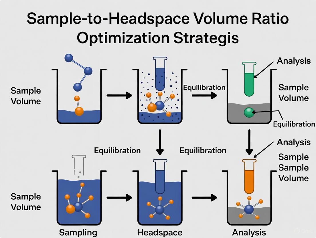
The entire process of static headspace analysis is governed by the goal of achieving a thermodynamic equilibrium between the analyte concentration in the sample phase and the gas phase [3]. The following diagram illustrates this process and the key parameters influencing the final result.

The fundamental relationship between the original sample concentration and the concentration detected by the GC is described by the following equation [2] [4] [5]:

CG = C0 / (K + β)

Where:

• C_G: Concentration of the analyte in the gas phase (headspace)
• C_0: Original concentration of the analyte in the sample
• K: Partition coefficient (CS / CG), representing the ratio of the analyte's concentration in the sample phase to its concentration in the gas phase at equilibrium [5]
• β: Phase ratio (VG / VL), the ratio of the headspace gas volume to the sample liquid volume [2]

The detector response (peak area, A) is directly proportional to C_G. Therefore, to maximize sensitivity, the sum (K + β) must be minimized [2]. The variables K and β are the primary levers for method optimization.

Key Optimization Parameters and Experimental Protocols

Optimizing a static headspace method involves systematically investigating several interdependent parameters. The following table summarizes the key parameters and their effects on the analysis.

Table 1: Key Parameters for Optimizing Static Headspace Analysis

Parameter	Effect on Analysis	Optimization Guidelines	Experimental Protocol
Sample Volume & Phase Ratio (β) [2] [4]	A lower β (more sample, less headspace) increases C_G for analytes with low K values. Has minimal effect for high K analytes.	Use a 10 mL sample in a 20 mL vial (β=1) as a starting point. Ensure at least 50% headspace remains [2] [6].	Method: Prepare a series of vials with increasing sample volumes (e.g., 2, 5, 10 mL) in 20 mL vials, keeping C_0 constant. Analysis: Inject and compare peak areas. The volume yielding the highest response for the target analytes is optimal.
Equilibration Temperature [2] [4] [3]	Increasing temperature decreases K for most analytes, driving them into the headspace and improving sensitivity.	Set oven temperature to ~20°C below the solvent's boiling point [6]. Accuracy of ±0.1°C is critical for precise results with high K analytes [4].	Method: Analyze identical samples at different equilibration temperatures (e.g., 40, 60, 80°C) for a fixed time. Analysis: Plot peak area vs. temperature. The point where the response plateaus is optimal. Monitor for analyte degradation.
Equilibration Time [4] [3]	Time required for analytes to reach equilibrium between the sample and gas phase. Insufficient time causes poor reproducibility.	Must be determined experimentally for each analyte/matrix combination. Agitation can significantly reduce the time required [3].	Method: Analyze identical samples with increasing equilibration times (e.g., 5, 10, 20, 30, 45 min) at a fixed temperature. Analysis: Plot peak area vs. time. The minimum time after which the area becomes constant is the optimal equilibration time.
Salting-Out [4] [5] [6]	Adding salt to aqueous samples reduces the solubility of polar analytes (decreases K), pushing them into the headspace.	Saturate the aqueous sample with a salt like potassium chloride or sodium chloride [5]. Test for unwanted co-extraction of matrix compounds [6].	Method: Prepare sample aliquots with different concentrations of salt (0%, 10%, 25%, saturation). Analysis: Compare peak areas. Salt concentration giving the highest response without increasing interference is optimal.

The Role of the Partition Coefficient (K)

The partition coefficient is a critical factor. Its value dictates how an analyte will respond to changes in other parameters [5]:

• High K value (~500): Indicates the analyte favors the sample phase (e.g., ethanol in water). For such analytes, increasing the temperature is the most effective way to improve headspace concentration, while increasing sample volume has little effect [4].
• Low K value (~0.01): Indicates the analyte strongly favors the gas phase (e.g., hexane in water). For these, increasing the sample volume provides a significant boost to C_G [4].

The Scientist's Toolkit: Essential Research Reagents and Materials

Table 2: Essential Materials for Static Headspace Analysis

Item	Function	Key Considerations
Headspace Vials	Container for sample and headspace gas [2].	Common sizes are 10 mL and 20 mL. Choose size based on desired phase ratio (β).
Septra & Caps	Provides a gas-tight seal for the vial [2].	Must be compatible with high incubation temperatures to prevent degradation and leakage [3] [6].
Non-Volatile Salts (e.g., KCl, NaCl)	Used for "salting-out" to improve volatility of polar analytes in aqueous matrices [4] [6].	Purity is critical to avoid introducing contaminants. Efficiency is salt and analyte-specific.
Headspace Syringe / Autosampler	To withdraw and inject a precise aliquot of the headspace gas [3].	Automated systems provide superior precision and accuracy compared to manual injection.
Narrow Bore GC Inlet Liner	The interface where the sample is introduced into the GC [6].	A narrow bore liner (e.g., 1.2 mm ID) prevents band broadening, resulting in sharper peaks and better signal [6].

Troubleshooting Common Static Headspace Issues: FAQs

Q1: My analysis is suffering from poor sensitivity. What are the primary parameters I should adjust? [7] [8]

• Increase Incubation Temperature: This is the most effective step for analytes with high partition coefficients (K), as it drives more analyte into the headspace [2] [4].
• Adjust Phase Ratio (β): For analytes with low K values, increasing the sample volume in a given vial will lower β and increase the signal [2] [4].
• Employ Salting-Out: For polar analytes in aqueous solutions, saturating the sample with salt can dramatically decrease K and improve sensitivity [4] [6].
• Check Instrument Settings: Ensure the sample transfer line and valve temperatures are at least 20°C hotter than the incubation oven to prevent sample condensation, which causes loss of analyte [4] [6].

Q2: I am seeing inconsistent (poor precision) results between replicate samples. What could be the cause? [3] [8]

• Insufficient Equilibration Time: Ensure the method allows enough time for the slowest analyte to reach equilibrium. This must be determined experimentally [4] [3].
• Poor Temperature Control: The equilibration oven must have excellent temperature stability (±0.1°C for high K analytes). Verify calibration regularly [4] [3].
• Variable Sample Volume/Vial Size: Inconsistent sample pipetting or using different vial sizes will change the phase ratio (β), leading to irreproducible results. Standardize volumes and vials [2].
• Leaky Vials: Ensure caps are crimped correctly and consistently, and that septa are not compromised by excessive temperature or needle punches [3] [6].

Q3: My chromatogram shows broad peaks or peak splitting. How can I resolve this? [3] [6]

• Use a Narrow Bore Inlet Liner: This is a common solution. A liner with a small internal diameter (e.g., 1.2 mm) reduces band broadening and sharpens peaks [6].
• Apply Inlet Splitting: If sensitivity allows, using a split injection (e.g., 10:1 split ratio) can improve peak shape and reproducibility [4] [6].
• Optimize Pressurization: In automated systems, a reverse flow of gas upon needle insertion can cause an early, partial injection, leading to peak splitting. Optimize pressurization delay and pressure to ensure a single, sharp injection [3].

Q4: When should I consider using Dynamic Headspace over Static Headspace? [1] [7]

Static headspace is simple and robust for many applications. However, consider dynamic headspace (DHS) when:

• Analyzing trace-level compounds requiring superior sensitivity, as DHS concentrates analytes on a trap [1] [7].
• Dealing with complex solid matrices or polar analytes in polar matrices that static headspace cannot efficiently extract [7].
• The target analytes have very low volatility and are not effectively transferred to the headspace under standard static conditions [7].

In static headspace gas chromatography (HS-GC), the phase ratio (β) is a fundamental design parameter that critically influences the sensitivity, precision, and overall success of the analytical method. For researchers and scientists optimizing sample-to-headspace volume ratios, a precise understanding of β is indispensable. This guide provides a detailed definition of the phase ratio, explores its role within the headspace system, and offers practical troubleshooting and optimization protocols to enhance method development for drug development professionals.

What is the Phase Ratio (β) in Headspace Analysis?

The phase ratio (β) is defined as the ratio of the volume of the gas phase (VG) to the volume of the liquid sample phase (VL) in a sealed headspace vial [9].

β = VG / VL

This ratio is a key determinant of the concentration of an analyte in the headspace gas (CG) at equilibrium, and consequently, of the signal intensity measured by the gas chromatograph [9]. The relationship between the original sample concentration (C0), the gas-phase concentration (CG), the partition coefficient (K), and the phase ratio (β) is given by the fundamental headspace equation [9] [4]:

C_G = C₀ / (K + β)

• C_G: Concentration of the analyte in the gas phase (headspace)
• C₀: Original concentration of the analyte in the liquid sample
• K: Partition coefficient (K = C_S/C_G), which is the ratio of the analyte's concentration in the sample phase (C_S) to its concentration in the gas phase at equilibrium [9]
• β: Phase ratio (V_G/V_L)

The following diagram illustrates the core relationships within a headspace vial that determine analyte concentration.

Troubleshooting Common Phase Ratio and Headspace Issues

FAQ: Addressing Frequent Challenges

1. My analysis shows poor repeatability (large variability in peak areas). Could the phase ratio be involved? While poor repeatability is often linked to temperature inconsistencies or vial leaks, an inconsistent sample volume directly changes the phase ratio (β) from vial to vial, leading to variable headspace concentrations [10] [9].

• Solution: Standardize your sample preparation procedure. Use precise, automated pipettes to ensure the same sample volume (VL) is introduced into every vial. This maintains a constant β and improves precision [10].

2. I am getting low peak areas for a soluble analyte. How can I improve sensitivity? For analytes with a high partition coefficient (K >> β), which are highly soluble in the sample matrix, simply increasing the sample volume (and thus decreasing β) has a negligible effect on the headspace concentration [4]. The system is dominated by the partition coefficient.

• Solution: Increase the incubation temperature to decrease the value of K, which will drive more analyte into the headspace [4]. Alternatively, use salting-out techniques (e.g., adding NaCl) to reduce the solubility of polar analytes in aqueous matrices [11] [4] [7].

3. For my insoluble analyte, the signal is weak. Will increasing the sample volume help? Yes. For analytes with a low partition coefficient (K << β), which have low solubility in the matrix, increasing the sample volume (decreasing β) will result in a significant, nearly proportional increase in the headspace concentration (CG) and a stronger signal [4].

4. What is the risk of using a very small sample volume in a large vial? A very small VL creates a large phase ratio (β). According to the equation CG = C0 / (K + β), a large β can lead to a very low headspace concentration (CG) for all analytes, potentially resulting in poor sensitivity and signals that are below the detection limit of your instrument.

Experimental Protocols for Phase Ratio Optimization

Protocol 1: Systematic Optimization of Sample Volume and Phase Ratio

This protocol is designed to empirically determine the optimal sample volume for maximizing sensitivity for your specific analytes.

1. Objective: To determine the effect of sample volume (VL) and the resulting phase ratio (β) on the chromatographic peak area of target analytes.

2. Research Reagent Solutions:

Item	Function in the Experiment
20 mL Headspace Vials	Standard enclosure for maintaining equilibrium between liquid and gas phases.
PTFE/Silicone Septa & Crimp Caps	Ensure a gas-tight seal to prevent analyte loss.
Automated Liquid Handler	Provides highly precise and reproducible sample volume transfers.
Sodium Chloride (NaCl)	"Salting-out" agent used to improve partitioning of polar analytes into the gas phase [11] [12].
Internal Standard	A compound added in constant amount to all vials to correct for instrumental variability.

3. Methodology: a. Prepare a standard solution of your target analytes at a concentration relevant to your application. b. Using an automated pipette or liquid handler, dispense this standard solution into a series of 20 mL headspace vials at different volumes (e.g., 0.5, 1.0, 2.0, 5.0, and 10.0 mL). For consistency, keep the concentration of any added salt or solvent constant. c. Seal all vials immediately. d. Analyze all samples using the same, controlled HS-GC method (constant temperature, equilibration time, etc.). e. Measure the peak areas for each analyte at each sample volume.

4. Data Analysis: Plot the peak area of each analyte against the sample volume (VL) or the calculated phase ratio (β = (20 - VL)/VL). The optimal volume is the one that provides the best sensitivity without negatively impacting the separation or the linearity of the method. The data can be summarized as follows:

Table 1: Sample Data for Phase Ratio Optimization (Theoretical Data)

Sample Volume (VL in mL)	Phase Ratio (β)	Peak Area - Analyte A (High K)	Peak Area - Analyte B (Low K)
0.5	39.0	1,500	85,000
1.0	19.0	2,900	89,500
2.0	9.0	5,100	92,000
5.0	3.0	9,800	94,800
10.0	1.0	12,500	96,200

Protocol 2: Investigating the Interaction of Temperature and Phase Ratio

This protocol uses a Design of Experiments (DoE) approach to efficiently understand interactive effects.

1. Objective: To model the interactive effects of equilibration temperature and sample volume/phase ratio on extraction efficiency.

2. Methodology: a. As demonstrated in a 2025 study on volatile petroleum hydrocarbons, a Central Composite Face-centered (CCF) design can be employed [11]. b. Select two factors: Equilibration Temperature (e.g., low: 40°C, center: 60°C, high: 80°C) and Sample Volume (e.g., low: 2 mL, center: 5 mL, high: 8 mL). c. The experimental software (e.g., Minitab) will generate a series of runs with different combinations of these two factors. d. The response variable is the chromatographic peak area, normalized per microgram of analyte [11]. e. Execute the experiments and use analysis of variance (ANOVA) to identify significant main and interaction effects.

3. Expected Outcome: The model will reveal whether temperature and phase ratio act independently or synergistically. For example, it may show that for a soluble analyte (high K), increasing temperature is the most critical factor, while for an insoluble analyte (low K), optimizing the sample volume is more impactful.

Key Optimization Parameters and Their Effects

Table 2: Guide to Parameter Optimization Based on Analyte Type

Parameter	Effect on System	Recommendation for High K (Soluble) Analytes	Recommendation for Low K (Insoluble) Analytes
Sample Volume (VL)	Directly sets the phase ratio (β).	Minimal impact on sensitivity. Use a consistent, moderate volume (e.g., 5-10 mL in a 20 mL vial) [4].	Critical. Increase sample volume (decrease β) for a significant sensitivity gain [4].
Equilibration Temperature	Decreases the partition coefficient (K).	Critical. Increase temperature to drive more analyte into the headspace. Requires very precise control (±0.1°C) for good precision [9] [4].	Lesser effect. Increasing temperature may have a minor or even slightly negative impact.
Salting-Out	Reduces K for polar analytes in aqueous matrices.	Highly recommended. Adding salts like KCl or NaCl improves volatility and sensitivity [4] [12] [7].	Not typically required, as analyte is already volatile.
Agitation	Increases mass transfer, reducing equilibration time.	Use to speed up analysis, especially for viscous samples [7].	Use to speed up analysis.

Frequently Asked Questions (FAQs)

What is the partition coefficient (K) in headspace analysis? The partition coefficient (K) is a fundamental equilibrium constant in static headspace gas chromatography (HS-GC). It is defined as the ratio of an analyte's concentration in the sample (liquid or solid) phase to its concentration in the gas (headspace) phase at equilibrium: K = C~S~/C~G~, where C~S~ is the concentration in the sample phase and C~G~ is the concentration in the gas phase [13] [4]. A high K value indicates that the analyte is more soluble in the sample matrix and has a lower tendency to partition into the headspace, whereas a low K value suggests high volatility and a greater presence in the gas phase.

How does the partition coefficient (K) differ from the distribution coefficient (D)? The partition coefficient, often denoted as log P, refers specifically to the concentration ratio of the un-ionized form of a compound between two phases. In contrast, the distribution coefficient (D, or log D) represents the ratio of the sum of the concentrations of all forms of the compound (ionized plus un-ionized) in each of the two phases. Therefore, log D is pH-dependent and provides a more comprehensive picture for ionizable compounds, whereas log P is constant for a given system [14] [15].

Why is understanding the partition coefficient critical for optimizing my headspace methods? The partition coefficient directly determines the analytical sensitivity of your headspace method. It governs the equilibrium concentration of an analyte in the headspace, which is what the GC instrument measures. A clear understanding of K allows you to predict how changes in method parameters (like temperature or sample volume) will affect the signal. Optimizing these parameters to minimize K for your analytes or to adjust the phase ratio (β) is the key to achieving high sensitivity and robust performance [13] [4].

How do temperature and sample volume affect the headspace equilibrium? The effects of temperature and sample volume are highly dependent on the value of the partition coefficient (K) [13] [4]. The relationship is summarized in the table below.

Table: Effect of Method Parameters Based on Analyte Partition Coefficient (K)

Method Parameter	Effect on Analytes with High K (e.g., Ethanol in water)	Effect on Analytes with Low K (e.g., Hexane in water)
Temperature Increase	Significantly increases headspace concentration. Requires very precise temperature control (±0.1°C) for good precision [4].	Minor effect; can sometimes even reduce headspace concentration.
Sample Volume Increase	Negligible effect on headspace concentration [4].	Significantly increases headspace concentration [4].

Troubleshooting Common Headspace Issues

Problem: Poor Repeatability (Large variability in peak areas)

• Possible Causes and Solutions:
  • Incomplete Equilibrium: Ensure sufficient incubation time (typically 15-30 minutes) to reach a stable gas-liquid equilibrium [10].
  • Temperature Instability: The vial thermostat temperature must be consistent and accurate. For analytes with high K, even a 1-2°C shift can cause a 10% change in peak area [13] [4]. Calibrate the heater and ensure vials are equilibrated fully.
  • Vial Leakage: Check for worn septa or overused caps. Always use certified vials and replace septa regularly [10].
  • Inconsistent Sample Prep: Standardize sample volume, salt addition, and agitation procedures to ensure identical matrix conditions across vials [10].

Problem: Low Peak Area or Reduced Sensitivity

• Possible Causes and Solutions:
  • High K Value / Low Volatility: The analyte may be too soluble in the sample matrix.
    • Solution: Increase the incubation temperature to drive more analyte into the gas phase [4] [10].
    • Solution: Use the "salting-out" effect by adding a high concentration of salt (e.g., KCl or NaCl) to the aqueous sample. This reduces the solubility of polar analytes, lowering K and increasing headspace concentration [4] [11].
    • Solution: For analytes with intermediate K values (~10), increasing the sample volume can improve headspace concentration [4].
  • System Leaks: Check for leaks in the vial septa, headspace sampling needle, transfer line, or inlet [10].

Problem: High Background or Ghost Peaks

• Possible Causes and Solutions:
  • Contamination: Contamination can originate from the injection needle, carrier gas, inlet liner, or even the vials themselves.
    • Solution: Run blank samples to identify the source. Clean the injection system regularly and use high-purity, pre-cleaned vials. Replace inlet liners and condition the column as needed [10].
  • Carryover: Ensure the autosampler needle is properly purged between samples. Increase the cleaning cycle or needle purge time if necessary [10].

Problem: Target Volatile Compounds Not Detected

• Possible Causes and Solutions:
  • Strong Matrix Binding: The analyte may be tightly bound to a solid or complex sample matrix.
    • Solution: Increase the incubation temperature and time to enhance release [10].
    • Solution: For solid samples, consider a phase transfer catalyst or switch to a dynamic headspace or SPME technique which can be more efficient for exhaustive extraction [13] [10].
    • Solution: Adjust the sample pH to convert ionic species into their neutral, more volatile form (e.g., for organic acids, lower the pH) [15].

Essential Experimental Protocols

Protocol: Determining the Optimal Equilibration Time

A critical step in any headspace method is ensuring the system has reached equilibrium.

• Preparation: Prepare multiple identical samples in headspace vials.
• Incubation: Place all vials in the autosampler and set a starting equilibration time (e.g., 5 minutes).
• Analysis: Analyze one vial and note the peak area of the target analyte.
• Iteration: Repeat the analysis on a new vial at progressively longer time intervals (e.g., 10, 20, 30, 40, 60 minutes).
• Determination: Plot the measured peak area versus equilibration time. The equilibration time is sufficient when the peak area reaches a stable plateau. Use this time, plus a small safety margin, for your final method [10].

Protocol: Optimizing Parameters via Experimental Design (DoE)

Traditional one-variable-at-a-time (OVAT) optimization is inefficient. A Design of Experiments (DoE) approach, as demonstrated in recent research, allows for the simultaneous optimization of multiple interacting parameters [11].

• Select Critical Factors: Identify key variables such as Incubation Temperature (°C), Equilibration Time (min), and Sample Volume (mL).
• Define Ranges: Set realistic low, medium, and high levels for each factor based on preliminary experiments.
• Create a Design Matrix: Use a statistical software package to generate an experimental design (e.g., a Central Composite Face-centered design). This dictates the specific combination of settings for each experimental run.
• Execute and Analyze: Run the experiments in the randomized order specified by the design. Use the chromatographic peak area as the response variable.
• Build a Model: Statistical analysis of variance (ANOVA) will identify which factors and their interactions have a significant impact on the response.
• Find the Optimum: The model can predict the combination of temperature, time, and sample volume that will yield the maximum peak area and sensitivity for your target analytes [11].

The following diagram illustrates the workflow for this systematic optimization process.

Diagram: Experimental Design for Headspace Optimization

The Scientist's Toolkit: Key Reagent Solutions

Table: Essential Materials for Headspace-GC Experiments

Item	Function / Explanation
n-Octanol & Water	Used to determine the octanol-water partition coefficient (K~ow~), a key predictor of a solute's lipophilicity/hydrophobicity and its partitioning behavior [14] [15].
Headspace Vials (20 mL)	Gas-tight vials with precise volumes to contain the sample and maintain equilibrium. Consistent vial volume is critical for controlling the phase ratio (β) [13].
PTFE/Silicone Septa & Crimp Caps	Provide a hermetic seal to prevent loss of volatile analytes and maintain pressure integrity during incubation and sampling [10] [11].
Sodium Chloride (NaCl) / Potassium Chloride (KCl)	Inorganic salts used for "salting-out." Their high concentration in aqueous samples reduces the solubility of organic analytes, lowering K and enhancing their concentration in the headspace [4] [11].
Internal Standards (e.g., deuterated analogs)	Compounds added in a constant amount to every sample and standard. Used to correct for analytical variability (injection volume, matrix effects) and improve quantitative accuracy.

The Fundamental Headspace Equation

In static headspace gas chromatography (HS-GC), the detector response is fundamentally governed by the equilibrium established between the sample and the vapor phase above it in a sealed vial. This relationship is described by the equation:

A ∝ C_G = C₀ / (K + β) [16] [13] [17]

Where:

• A is the peak area obtained from the GC detector, which is proportional to the analyte concentration in the gas phase (C_G) [16].
• C₀ is the original concentration of the analyte in the sample solution [16] [4].
• K is the partition coefficient (also called distribution coefficient), defined as K = C_S / C_G, representing the ratio of the analyte's concentration in the sample phase (C_S) to its concentration in the gas phase (C_G) at equilibrium [16] [13].
• β is the phase ratio, defined as β = V_G / V_S, which is the ratio of the volume of the headspace gas (V_G) to the volume of the sample (V_S) [16] [13].

To maximize the detector signal (A), the goal is to maximize C_G. This is achieved by minimizing the sum (K + β) in the equation's denominator [16] [17]. The following diagram illustrates the logical relationship between the headspace equation and the key parameters that influence it.

Troubleshooting Guides and FAQs

Common Problems and Solutions

Problem Symptom	Potential Cause	Diagnostic Steps	Solution
Low Sensitivity (Small peak areas) [6]	Analyte too soluble in matrix (High K) [13].	Check analyte polarity vs. matrix. Review K values if known.	Increase equilibration temperature [16] [13]. Use salting-out effect (add salt) [6] [4].
	Unfavorable phase ratio (High β) [16].	Calculate β (VG/VS). Is sample volume too small?	Increase sample volume to decrease β [16] [4].
Poor Precision (High %RSD) [4]	Inconsistent temperature control [13].	Monitor oven temperature stability.	Ensure precise and stable vial thermostatting [4].
	Leaky vials or inconsistent sealing [6].	Check crimp cap consistency; inspect septa.	Use quality vials/septa; ensure crimper is correctly adjusted [16] [6].
	Variable sample volume [17].	Review sample preparation pipetting technique.	Use precise liquid handling equipment; maintain consistent volume [17].
Long Equilibration Times	Low temperature or no agitation [16].	Check if peak areas plateau over time.	Optimize equilibration time experimentally; use vial shaking if available [16].
Peak Tailing	Sample condensation in transfer line [4].	Verify transfer line temperature.	Set transfer line temperature 20°C above oven temperature [4].

Frequently Asked Questions

Q1: How does temperature precisely affect the headspace analysis for different types of analytes? The effect is highly dependent on the analyte's solubility in the sample matrix (its K value) [13]. For analytes with high solubility (high K, like ethanol in water), even a small temperature increase significantly reduces K and dramatically increases the peak area. For these, temperature control must be very precise (±0.1 °C) [13] [4]. For analytes with low solubility (low K, like n-hexane in water), temperature has a much smaller effect on the peak area [13].

Q2: My sample volume is limited. How can I maintain good sensitivity? Using a smaller vial size is the most effective strategy. For example, transferring a 1 mL sample from a 20 mL vial (β=19) to a 10 mL vial (β=9) significantly reduces the phase ratio, thereby increasing C_G and sensitivity [16]. Ensure at least 50% of the vial volume is headspace for proper equilibration [16] [6].

Q3: What is the "salting-out" effect and when should I use it? Salting-out involves saturating an aqueous sample with a salt like sodium chloride. This reduces the solubility of polar organic analytes in the water, decreasing their K value and forcing more analyte into the headspace vapor, which increases sensitivity [6] [4]. It is most effective for polar analytes in aqueous matrices and may have little effect on analytes that already have a very low K [6].

Q4: Why is the solvent peak so small in headspace-GC compared to direct liquid injection? In headspace-GC, only the volatile components that have partitioned into the gas phase are introduced into the instrument. The bulk of the non-volatile or less-volatile solvent remains in the sample vial. This results in a much smaller solvent peak, minimizing its potential to interfere with the analysis of early-eluting target analytes [16] [18].

Experimental Protocol: Optimizing Headspace Parameters Using a DoE Approach

The following workflow outlines a robust methodology for optimizing headspace parameters, moving beyond the traditional one-variable-at-a-time approach to capture interaction effects [11].

Detailed Methodologies:

• Factor Definition: Identify and set realistic ranges for critical parameters. A typical screening experiment might include:

  • Sample Volume (V): For a 20 mL vial, test 2 mL, 5 mL, and 10 mL [16] [4].
  • Equilibration Temperature (T): Test a range, ensuring it stays ~20°C below the solvent's boiling point (e.g., 40°C, 60°C, 80°C for aqueous samples) [16] [13].
  • Equilibration Time (t): Test varying times (e.g., 10, 20, 30 min) to ensure equilibrium is reached [16].

• Experimental Design: Employ a multivariate design such as a Central Composite Face-Centered (CCF) design. This approach is efficient and allows for the modeling of curvature and interaction effects between parameters, which a one-variable-at-a-time approach would miss [11].

• Sample Preparation and Analysis:

  • Prepare standard solutions in the sample matrix (e.g., aqueous solutions for water analysis) [11].
  • Transfer defined sample volumes into headspace vials. For aqueous samples, add a consistent amount of salt (e.g., 1.8 g NaCl) if the salting-out effect is being investigated [11] [6].
  • Seal vials immediately with PTFE/silicone septa and aluminum crimp caps [11].
  • Analyze vials in random order according to the experimental design matrix using an automated headspace autosampler coupled to GC-FID or GC-MS [11].

• Data Analysis: Use the chromatographic peak area per microgram of analyte as the response variable. Perform Analysis of Variance (ANOVA) on the data to determine the global significance of the model and identify which factors and interactions have a statistically significant impact on the extraction efficiency [11].

The Scientist's Toolkit: Essential Research Reagents and Materials

Item	Function	Application Notes
Headspace Vials	Container for sample and headspace gas during equilibration [16].	Common sizes are 10 mL and 20 mL. Choose vial size based on required sample volume and desired phase ratio (β) [16].
PTFE/Silicone Septa & Caps	Provides a gas-tight seal to prevent loss of volatile analytes [16] [6].	Must withstand incubation temperature without degrading. Ensure caps are crimped tightly and consistently [6].
Sodium Chloride (NaCl)	Used to induce the "salting-out" effect in aqueous samples [11] [6].	Saturating the sample with salt reduces K for polar analytes, enhancing sensitivity [4].
Non-Polar GC Column	Separates vaporized analyte components prior to detection [11] [18].	e.g., DB-1 or equivalent with (5%-phenyl)-methylpolysiloxane stationary phase, suitable for volatile hydrocarbons [11].
Narrow Bore Inlet Liner	Interface for transferring the headspace vapor into the GC column [6].	A narrow internal diameter (e.g., 1.2 mm) helps prevent band broadening, resulting in sharper peaks [6].

How Sample Matrix Influences Activity Coefficients and Volatility

Frequently Asked Questions (FAQs)

Q1: What is the sample matrix and why is it critical in headspace analysis? The sample matrix encompasses everything in the sample except for the target analytes. This includes the solvent, salts, proteins, and other co-extracted compounds [19]. It is critical because the matrix components can significantly affect the activity coefficient (γ) of an analyte, which is a measure of the intermolecular attraction between the analyte and the other species within the sample [4]. A change in the activity coefficient directly alters an analyte's vapor pressure and its partitioning between the liquid sample and the headspace gas, thereby influencing the final concentration measured by the GC instrument [4] [20].

Q2: How does the sample matrix physically affect an analyte's volatility? The matrix influences volatility through chemical interactions. In a headspace vial, the concentration of an analyte in the gas phase (C~G~) is related to its concentration in the original sample (C~0~) by the partition coefficient (K) and the phase ratio (β), which is the ratio of the headspace volume to the sample volume (V~G~/V~L~) [4] [21]. The fundamental relationship is described by:

A ∝ C~G~ = C~0~ / (K + β) [21]

The partition coefficient K is itself inversely proportional to the analyte's vapor pressure and its activity coefficient (γ) in the matrix [4]. Therefore, a matrix that increases the activity coefficient (e.g., by "salting out") will decrease the partition coefficient K, driving more analyte into the headspace and increasing the detector response [21] [20].

Q3: My analyte recovery is low. How can I modify the sample matrix to improve volatility? Low recovery often indicates that your analyte is too soluble in the sample matrix (a high partition coefficient, K). You can modify the matrix to reduce solubility and increase the activity coefficient using these strategies [4] [21] [22]:

• Salting-Out: For polar analytes in aqueous matrices, adding a high concentration of a salt like potassium chloride (KCl) can significantly reduce the partition coefficient. This "salting out" effect decreases the solubility of the analyte in the aqueous phase, forcing more into the headspace [4] [22].
• Solvent Adjustment: For solid samples, adding a small amount of solvent can sometimes create more favorable partition coefficients. Conversely, for analytes in a solvent, changing to a solvent with which the analyte has less favorable interactions can increase its activity coefficient [21].
• pH Adjustment: For analytes that can be ionized (e.g., acids or bases), adjusting the pH to suppress ionization can convert the analyte into a more volatile, neutral form, dramatically increasing its presence in the headspace.

Q4: How do I choose the right matrix for calibration standards? It is crucial to use a matrix-matched calibration for accurate quantification [4] [19]. The standard should be prepared in a blank matrix that is identical to your sample, minus the analyte. This accounts for any matrix-induced enhancement or suppression of the analyte signal [19]. For a drug product, this means using a placebo with all excipients. For bioanalytical methods, guidelines suggest testing blank matrix from at least six different sources to check for interferences [19].

Troubleshooting Guide

Symptom	Possible Cause	Solution
Low detector signal / poor sensitivity	High solubility of analyte in matrix (Low activity coefficient).	Apply "salting-out" by saturating the aqueous sample with salt [4] [22]. Increase incubation temperature [4] [21]. Increase sample volume (for analytes with low K) [4].
Poor precision and accuracy	Inconsistent sample matrix between standards and samples.	Use matrix-matched calibration standards [4] [19]. Ensure consistent sample volume and vial size to maintain a constant phase ratio (β) [21].
	Incomplete equilibrium due to complex matrix.	Increase equilibration time and use vial agitation if available [4] [21].
Unidentified interference peaks in chromatogram	Endogenous compounds from sample matrix co-eluting with analyte.	Demonstrate method specificity by analyzing a blank matrix [19]. Optimize GC separation parameters or use a more selective detector (e.g., MS) [19].
Nonlinear calibration curve	Saturation of the headspace or active sites in the matrix at high concentrations.	Reduce sample concentration or volume. Use internal standard calibration.

Experimental Parameters and Optimization Strategies

The following table summarizes key experimental parameters you can adjust to counteract matrix effects and optimize the transfer of analyte from the sample to the headspace.

Table 1: Key Experimental Parameters for Optimizing Headspace Analysis

Parameter	Influence on Activity Coefficient & Volatility	Optimization Guideline
Salt Addition	Significantly increases activity coefficient (γ) of polar analytes in aqueous matrices, reducing their solubility and driving them into the headspace [4] [20] [22].	Use high-purity salts (e.g., KCl, NaCl). Saturation of the aqueous phase is typical. Test effectiveness for your specific analyte-matrix combination [4].
Temperature	Increasing temperature decreases the partition coefficient (K) for most analytes, increasing headspace concentration. Precision requires highly accurate temperature control (±0.1°C for high K analytes) [4] [21].	Set oven temperature as high as possible but remain at least 20°C below the solvent boiling point to avoid excessive pressure [4] [21].
Sample Volume (Phase Ratio, β)	Increasing sample volume decreases the phase ratio (β = V~G~/V~L~), which increases C~G~ for analytes with low K values. For high K values, the effect is minimal [4] [21].	Use a consistent vial size. For a 20-mL vial, 10 mL of sample gives a phase ratio of 1, which simplifies calculations. Always leave at least 50% headspace [4] [21].
Equilibration Time	Does not directly change activity coefficient but is required for the system to reach a stable equilibrium where the headspace concentration is reproducible [4].	Determine experimentally for each analyte-matrix combination. It depends on vapor pressure, agitation, and temperature [4] [21].

Detailed Experimental Protocol: Matrix Modification via Salting-Out

Title: Determination of Ethanol in Blood Using Static Headspace-GC-MS with Matrix-Matched Calibration and Salting-Out

1. Principle This method uses the addition of salt to the aqueous blood sample matrix to increase the activity coefficient of ethanol, reducing its partition coefficient and enhancing its concentration in the headspace for improved detection [4] [21]. Matrix-matched calibration ensures accurate quantification by accounting for other matrix effects [19].

2. Materials and Reagents

• Internal Standard Solution: 1-Butanol or n-propanol in ultrapure water.
• Salting Agent: High-purity Potassium Chloride (KCl).
• Calibration Standards: Ethanol, certified reference material.
• Blank Matrix: Ethanol-free human blood or appropriate surrogate.
• Headspace Vials: 20 mL, crimp-top with PTFE/silicone septa.
• Gas Chromatograph-Mass Spectrometer (GC-MS): Equipped with a static headspace autosampler.

3. Procedure 3.1. Sample Preparation

• Pipette 1.0 mL of blood sample, calibration standard, or blank matrix into a 20 mL headspace vial.
• Add 100 µL of internal standard solution and 2.0 g of solid KCl.
• Immediately cap the vial and vortex vigorously for 30 seconds to dissolve the salt and homogenize the mixture.

3.2. Calibration Curve Preparation

• Prepare a stock solution of ethanol in blank matrix.
• Serially dilute with blank matrix to create at least five calibration levels covering the expected concentration range (e.g., 0.01 - 1.0 mg/mL).
• Prepare each calibration level according to the steps in Section 3.1.

3.3. Headspace-GC-MS Analysis

• Incubation: Load vials into the autosampler and incubate at 70°C for 15 minutes with agitation [23].
• Injection: Use a sample loop (e.g., 1 mL) to inject the headspace gas from each vial.
• GC Conditions:
  • Column: Mid-polarity capillary column (e.g., 30 m × 0.25 mm ID, 0.25 µm film thickness).
  • Oven Program: 40°C (hold 2 min), ramp at 15°C/min to 120°C.
  • Carrier Gas: Helium, constant flow of 1.0 mL/min.
• MS Detection:
  • Ionization Mode: Electron Impact (EI) at 70 eV.
  • Acquisition Mode: Selected Ion Monitoring (SIM) for ethanol (m/z 31, 45) and the internal standard.

4. Data Analysis

• Plot the peak area ratio (analyte / internal standard) against the known concentration for each calibration standard to generate the calibration curve.
• Use the linear regression equation from the curve to calculate the concentration of ethanol in the unknown samples.

Research Reagent Solutions

Table 2: Essential Materials for Headspace Analysis

Item	Function	Example & Specification
Salting-Out Reagents	Increases activity coefficient of polar analytes, improving volatility and sensitivity [4] [22].	Potassium Chloride (KCl), Sodium Chloride (NaCl), Anhydrous, high purity (>99%) [4].
Internal Standards	Corrects for variability in sample preparation, injection, and matrix effects, improving quantitative accuracy [23].	Deuterated analogs of the analyte (e.g., CD~3~CD~2~OH for ethanol) or compounds with similar chemical behavior (e.g., 1-Butanol) [23].
Matrix-Matched Blank	Serves as the foundation for calibration standards and specificity testing, ensuring accuracy by mimicking the sample's chemical environment [19].	Analyte-free blood, urine, placebo drug formulation, or artificial soil/water.
Headspace Vials & Seals	Provides a sealed, inert environment for sample equilibration, preventing loss of volatile analytes [21].	20 mL glass vials with aluminum crimp caps and PTFE/silicone septa to ensure a pressure-tight seal [21] [23].

Workflow and Logical Relationships

The following diagram illustrates the logical sequence of how the sample matrix influences the final analytical signal in headspace GC, and the primary parameters available for optimization.

Practical Application: Implementing Volume Ratio Optimization in Method Development

Frequently Asked Questions

1. What is the "50% Headspace Rule" and why is it important? The "50% Headspace Rule" is a general guideline suggesting that when preparing a headspace vial, you should fill it so that approximately 50% of the vial's capacity is occupied by the sample, leaving the remaining 50% as headspace [24]. This rule is crucial because it ensures a sufficient vapor phase volume for analyte detection while maintaining an optimal phase ratio (β), which is the ratio of headspace volume (VG) to sample volume (VL) [25] [4]. A properly balanced phase ratio is fundamental for achieving consistent and sensitive analytical results, as it directly influences the concentration of volatile compounds in the headspace available for injection into the GC system [25].

2. When should I deviate from the 50% rule? While the 50% rule is an excellent starting point, you should deviate from it when dealing with specific analytical challenges. For analytes with very low partition coefficients (K), meaning they have a high tendency to escape into the headspace (like hexane in water), increasing the sample volume significantly boosts the headspace concentration [4]. Conversely, for analytes with very high K values, which prefer to stay in the liquid phase (like ethanol in water), increasing the sample volume has a minimal effect on headspace concentration [4]. In such cases, increasing the equilibration temperature is a more effective strategy for improving sensitivity [4].

3. My headspace sensitivity is low. How can I improve it? Low sensitivity can be addressed by optimizing several key parameters:

• Increase Sample Volume: For analytes with low K values, using a larger sample volume in a larger vial (e.g., 10 mL of sample in a 20-mL vial) can enhance the signal [4].
• Raise Equilibration Temperature: Carefully increasing the temperature can drastically reduce the partition coefficient for many analytes, driving more molecules into the headspace [25] [26]. Ensure the temperature stays about 20°C below the solvent's boiling point [25].
• Add Salt ("Salting Out"): Adding a high concentration of salt (e.g., potassium chloride) to the sample matrix can reduce the solubility of polar analytes in a polar solvent like water, forcing them into the headspace [4] [27].
• Optimize Equilibration Time: Ensure the vial is heated for a sufficient, experimentally determined time to allow the system to reach a full equilibrium [26].

4. I'm getting poor reproducibility between samples. What could be wrong? Poor reproducibility often stems from inconsistencies in sample handling or method parameters:

• Inconsistent Sample Volume or Vial Type: Using different sample volumes or different vial sizes between runs alters the phase ratio, leading to variable results. Standardize these parameters [24].
• Improper Sealing: Ensure crimp caps are properly sealed or screw caps are uniformly tightened to prevent leaks [24] [28].
• Variable Equilibration Temperature or Time: Precise temperature control (within ±1–2 °C) is critical for good precision, especially for analytes with high K values [26] [4]. Equilibration time must be sufficient and consistent for all samples.
• Sample Handling: Volatile compounds can be lost during sample preparation. Handling samples at reduced temperatures and using consistent techniques can improve repeatability [26].

Troubleshooting Common Problems

Problem	Possible Cause	Solution
Low Peak Area	Sample volume too small for analytes with low K [4].	Increase sample volume and use a larger vial [25].
	Temperature too low [25].	Increase equilibration temperature [4].
	Equilibrium not reached [26].	Increase equilibration time; use agitation if available [26].
Poor Precision	Inconsistent sample volumes [24].	Use automated pipettes for accurate dispensing.
	Variable vial temperatures [26].	Service and calibrate the headspace sampler oven.
	Leaking vial seals [28].	Check septa for compatibility, use crimp caps for the tightest seal [28].
Carryover or Contamination	Contaminated sampler needle or transfer line.	Implement a robust needle and system purge routine.
Split Peaks or Double Peaks	Natural vial pressure too high, causing a reverse pulse upon needle insertion [26].	Reduce equilibration temperature or use a pressure-release cap [26] [28].

Key Optimization Parameters and Their Effects

The following table summarizes the main parameters to optimize for an efficient headspace analysis, based on the equation CG = C0/(K + β), where the detector response is proportional to the concentration in the gas phase (CG) [25] [4].

Parameter	Effect on Headspace Concentration	Recommendation & Rationale
Sample Volume & Vial Size (Phase Ratio, β)	Has a major effect. For low K analytes, increasing sample volume strongly increases CG. For high K analytes, the effect is minimal [4].	Start with the 50% rule (e.g., 10 mL sample in a 20 mL vial, β=1) [24] [4]. Adjust based on analyte K: use more sample for volatile analytes (low K).
Equilibration Temperature	Has a major effect. Increasing temperature typically decreases K, thereby increasing CG [25] [4].	Use an elevated temperature (at least 15°C above room temp) [26]. Balance between sensitivity and analyte/matrix stability. Do not exceed septum temperature limits [26].
Equilibration Time	Must be sufficient to reach equilibrium. Time is analyte- and sample-dependent [26] [4].	Determine experimentally. Use agitation to significantly reduce the time required to reach equilibrium [26].
Salting Out	Adding salt decreases K for polar analytes in polar matrices, increasing CG [4] [27].	Use high concentrations of salts like KCl or (NH₄)₂SO₄ for analytes in aqueous matrices [4] [27].

Experimental Protocol: Optimizing Sample Volume and Vial Size

This protocol provides a systematic methodology for empirically determining the optimal sample volume and vial size for a specific application, a critical part of thesis research on volume ratio optimization.

1. Principle To maximize detector response by finding the sample volume and vial size combination that minimizes the sum (K + β) in the fundamental headspace equation, thereby maximizing the concentration of the target analyte in the gas phase (CG) [25] [4].

2. Materials

• Analytical Instrumentation: Gas Chromatograph equipped with a headspace autosampler (e.g., valve-and-loop system) and a suitable detector (FID, MS) [29] [25].
• Vials: Headspace vials of different volumes (e.g., 10 mL and 20 mL) with matching crimp or screw caps and inert septa (e.g., PTFE/silicone) [24] [28].
• Chemicals: Standard solution of the target analyte(s) in the appropriate matrix. For quantitative studies, use internal standards if available [29].

3. Procedure

• Step 1: Standard Preparation. Prepare a calibration series of your target analyte at different concentrations in the relevant sample matrix.
• Step 2: Sample Loading. For each concentration level, prepare headspace vials in triplicate using different sample volumes. A typical experimental setup is shown below [25]:
  • 20 mL Vials: Load 2 mL, 5 mL, 10 mL, and 15 mL of sample.
  • 10 mL Vials: Load 1 mL, 3 mL, 5 mL, and 7 mL of sample.
• Step 3: Sealing. Wipe the vial rims clean and seal them securely using a crimper or by tightening screw caps to a uniform torque [24].
• Step 4: Equilibration and Analysis. Place the vials in the autosampler and run the sequence using a consistent, pre-optimized method (temperature, time, etc.) [26].
• Step 5: Data Analysis. Plot the average peak area (or height) for the target analyte against the sample volume for each vial size.

4. Expected Outcome You will identify the sample volume and vial size that produces the highest detector response for your analyte, effectively optimizing the phase ratio for your specific system.

The Scientist's Toolkit: Essential Research Reagents & Materials

Item	Function & Rationale
Headspace Vials (Borosilicate Glass)	Inert containers that withstand heating and pressure. Sizes (10, 20 mL) allow for phase ratio optimization [25] [24]. Amber vials protect light-sensitive samples [28].
Septa (PTFE/Silicone or PTFE/Butyl)	Provide a resealable, inert barrier. PTFE/Butyl offers superior chemical resistance. High-temp septa are available for demanding methods [28].
Crimp Caps (Aluminum)	Provide the most secure, leak-proof seal, essential for maintaining equilibrium and achieving high reproducibility [24] [28].
Salting Agents (e.g., KCl)	"Salt out" polar analytes from aqueous matrices by reducing their solubility, thereby increasing their headspace concentration and improving sensitivity [4] [27].
Internal Standards (Deuterated Analogs)	Added in known amounts to correct for losses and variability during sample preparation and analysis, crucial for accurate quantification [29].

Workflow Diagram: Headspace Method Optimization

The following diagram illustrates the logical decision process for optimizing the sample-to-headspace volume ratio and other key parameters.

Analyzing the Impact of Sample Volume on Analytes with High vs. Low K Values

FAQ: How does changing the sample volume in a headspace vial affect my results?

The effect is not uniform; it depends critically on the partition coefficient (K) of your target analyte [4]. The partition coefficient (K = C_liquid/C_gas) describes how an analyte distributes itself between the sample liquid and the headspace gas at equilibrium [30]. The relationship between the concentration in the headspace (C_G) and the original sample is governed by the equation: C_G = C₀ / (K + β), where β is the phase ratio (V_G/V_L) [4] [30] [31]. Changing the sample volume directly alters the phase ratio (β), which in turn affects the concentration of analyte available for injection into the GC [4] [30].

The table below summarizes the expected impact of increasing sample volume for different types of analytes.

Analyte Solubility & K Value	Partition Coefficient (K)	Impact of Increasing Sample Volume on Headspace Concentration
High Solubility / High K	K is large (e.g., ~500 for ethanol in water) [4]	Little to no significant increase [4]. The large K value dominates the denominator, making the effect of changing β negligible.
Intermediate Solubility / Intermediate K	K ~10 [4]	Approximately linear increase [4]. The headspace concentration rises in a roughly proportional manner with sample volume.
Low Solubility / Low K	K is small (e.g., ~0.01 for hexane in water) [4]	Large, proportional increase [4]. A small K value means the β term is more influential, so increasing sample volume significantly boosts the signal.

Troubleshooting Guide: Optimizing Sample Volume

Symptoms and Solutions

• Symptom: Low sensitivity for a very volatile analyte (e.g., a light hydrocarbon).

  • Potential Cause: The analyte has a very low K value and the sample volume is too small, resulting in a high, unfavorable phase ratio (β).
  • Solution: Increase the sample volume. For a 20 mL vial, using 10 mL of sample is a common and effective starting point, as it sets β=1 and simplifies calculations while maximizing sensitivity for low-K analytes [4] [30].

• Symptom: Low sensitivity for a semi-volatile, water-soluble analyte (e.g., ethanol).

  • Potential Cause: The analyte has a high K value. Increasing sample volume will not effectively improve sensitivity.
  • Solution: Increase the equilibration temperature to lower the K value, or employ salting-out techniques (e.g., saturating the aqueous sample with salt like potassium chloride or sodium chloride) to reduce the analyte's solubility and drive it into the headspace [4] [6] [11].

• Symptom: Inconsistent peak areas or poor precision.

  • Potential Cause: Inconsistent sample volumes or vial filling, leading to variable phase ratios between injections.
  • Solution: Use an autosampler if available and ensure precise, reproducible liquid dispensing. Consistently fill vials to at least 50% of their capacity to maintain a stable phase ratio [6].

Experimental Protocol: Determining Optimal Sample Volume

The following methodology, adapted from a recent study optimizing headspace for volatile hydrocarbons, provides a robust framework for your own investigations [11].

1. Objective To systematically determine the optimal sample volume for the headspace-GC analysis of specific target analytes in a given matrix.

2. Materials and Reagents

• Headspace Vials: 20 mL vials with PTFE/silicone septa and aluminum crimp caps [11].
• Matrix-Matched Standards: Prepare calibration standards in the same matrix as your sample (e.g., ultrapure water for environmental aqueous samples) to ensure accurate activity coefficients [4] [11].
• Salt for Salting-Out: High-purity salt, such as Sodium Chloride (NaCl) or Potassium Chloride (KCl) [4] [6] [11].

3. Instrumentation

• Gas Chromatograph equipped with a Flame Ionization Detector (FID) or Mass Spectrometer (MS).
• Static Headspace Autosampler (e.g., Agilent 7697A or similar) [11].
• Capillary GC Column (e.g., 30 m x 0.25 mm ID, non-polar stationary phase like 5% diphenyl/95% dimethyl polysiloxane) [11].

4. Procedure 1. Prepare a series of headspace vials spiked with the same concentration of your target analyte(s). 2. Systematically vary the sample volume across the vials (e.g., 2, 5, 10, 15 mL in a 20 mL vial), keeping all other parameters (analyte concentration, temperature, equilibration time) constant. 3. For aqueous samples, add a constant, high concentration of salt (e.g., 1.8 g of NaCl) to all vials to induce a salting-out effect and maintain consistent ionic strength [11]. 4. Crimp seal the vials immediately to prevent volatile loss. 5. Analyze the vials using your standardized HS-GC method. 6. Plot the chromatographic peak area (or area per μg of analyte) against the sample volume for each analyte [11].

5. Data Analysis The optimal sample volume is identified as the point where the response (peak area) reaches a plateau or begins to offer the best compromise between sensitivity and the practical need to maintain sufficient headspace (at least 50%) for reliable pressurization and sampling [6].

The Scientist's Toolkit: Essential Research Reagents and Materials

The table below lists key materials required for experiments on sample volume optimization.

Item	Function / Purpose
20 mL Headspace Vials	Standard container for sample incubation and equilibration; allows for a wide range of sample volumes to be tested [30].
PTFE/Silicone Septa & Aluminum Caps	Forms a gas-tight seal to prevent loss of volatile analytes during heating and pressurization [6] [11].
Sodium Chloride (NaCl), ACS Grade	A "salting-out" agent. Adding a high concentration of salt to aqueous samples reduces the solubility of polar analytes, lowering their K value and increasing headspace concentration [4] [6] [11].
Matrix-Matched Calibration Standards	Solutions of target analytes prepared in a solvent that closely mimics the sample matrix. Essential for accurate quantification as the matrix affects the analyte's activity coefficient [4].
Mechanical Crimper/Decapper	Tool to ensure caps are applied uniformly tight with no leaks, which is critical for reproducibility [6].

Method Optimization Decision Pathway

This diagram outlines the logical process for optimizing headspace methods based on analyte properties.

In the pharmaceutical industry, ensuring that residual solvents in drug products are below toxicologically accepted limits is a mandatory requirement for patient safety [32]. Static headspace gas chromatography (HS-GC) is the gold standard technique for this analysis. Within method development, optimizing the sample volume, or more precisely the sample-to-headspace volume ratio, is a fundamental step that directly impacts method sensitivity, accuracy, and robustness [4] [33]. This case study, framed within broader research on volume ratio optimization strategies, provides a detailed investigation into how sample volume affects the detection of residual solvents, complete with experimental data, troubleshooting guides, and optimized protocols for scientists in drug development.

The underlying principle is defined by the fundamental headspace equation [33]:

A ∝ CG = C0 / (K + β)

Where:

• A is the chromatographic peak area (detector response).
• CG is the analyte concentration in the gas phase.
• C0 is the original analyte concentration in the sample.
• K is the partition coefficient (concentration in sample / concentration in headspace).
• β is the phase ratio (volume of headspace gas / volume of sample liquid, VG/VL).

The goal of volume optimization is to minimize the denominator (K + β), thereby maximizing CG and the detector signal A. For analytes with a low K value (indicating high volatility and low solubility in the sample matrix), the phase ratio β becomes the dominant factor. A smaller β, achieved by increasing the sample volume or decreasing the headspace volume, leads to a higher concentration of the analyte in the headspace and a stronger signal [4] [33].

Experimental Protocol and Workflow for Volume Optimization

Research Reagent Solutions and Materials

The following table details the essential materials and reagents required to perform the experiments described in this case study.

Table 1: Essential Research Reagents and Materials

Item	Function/Justification
Active Pharmaceutical Ingredient (API) or Drug Product	The test material for which residual solvent levels need to be determined.
Headspace Grade Water, DMSO, DMF, or NMP	High-purity solvents used to dissolve or suspend the sample. The choice depends on the solubility of the drug substance [34].
Residual Solvent Mixtures (Class 1, 2, and 3)	Certified reference standard mixtures for instrument calibration, covering solvents like benzene, toluene, cyclohexane, 1,4-dioxane, and chloroform [32] [35].
Sodium Chloride (NaCl), Analytical Grade	A non-volatile salt used for the "salting-out" effect, which decreases the solubility of polar analytes in the aqueous phase, driving them into the headspace and improving sensitivity [4].
Headspace Vials (e.g., 10 mL, 20 mL)	Vials of different sizes are critical for experimentally determining the optimal phase ratio (β).
Gas Chromatograph	Equipped with a Flame Ionization Detector (FID) or Mass Spectrometer (MS).
Static Headspace Autosampler	An automated system, preferably a valve-and-loop design, for precise and reproducible sampling of the vapor phase [34] [33].

Detailed Volume Optimization Methodology

This protocol outlines a systematic approach to determine the optimal sample volume for residual solvent analysis.

Step 1: Standard and Sample Preparation

• Prepare a stock standard solution of target residual solvents in an appropriate headspace-grade solvent at a concentration relevant to the permitted daily exposure (PDE) limits [34].
• Spike a consistent amount of this stock solution into a series of headspace vials.
• To each vial, add a varying volume of the same solvent used for the stock solution (e.g., water) to create a set of standards with identical analyte mass but different sample volumes. For a 20 mL vial, typical volumes to test are 1, 2, 5, and 10 mL.

Step 2: Instrumental Analysis

• Analyze all prepared vials using a validated HS-GC method.
• Keep all chromatographic parameters (column, temperature program, detector) and headspace parameters (equilibration temperature, equilibration time, transfer line temperature) constant across all runs. The only variable should be the sample volume.
• Ensure the sample loop volume and pressurization time of the headspace autosampler are sufficient for reproducible injections [33].

Step 3: Data Analysis and Optimization

• For each target analyte, plot the chromatographic peak area (or peak height) against the sample volume.
• The optimal volume is identified as the point where the signal response plateaus or begins to decrease. A decreasing signal at high volumes can indicate overfilling, which reduces the headspace volume excessively and can lead to pressure issues or liquid pull-over [4].
• A best practice is to select a sample volume that provides at least 50% headspace in the vial to ensure a sufficient gas phase for sampling [33].

The following workflow diagram illustrates the logical decision process for volume optimization.

Results and Data Analysis

Quantitative Data from Volume Optimization

The data below, generated from a model experiment, demonstrates the impact of sample volume on detector response for three representative solvents with different partition coefficients (K) in water.

Table 2: Impact of Sample Volume on Analyte Peak Area (in a 20 mL Vial)

Sample Volume (mL)	Phase Ratio (β)	Benzene (Low K)	Ethanol (High K)	Toluene (Medium K)
2	9.0	1,250,000	45,000	850,000
5	3.0	2,850,000	95,000	1,750,000
10	1.0	4,150,000	450,000	2,900,000
15	0.33	3,900,000	440,000	2,850,000

Interpretation of Results:

• Benzene (Low K): As a highly volatile and poorly water-soluble solvent, it shows a dramatic signal increase as the sample volume increases and β decreases. The signal plateaus at 10 mL, indicating the optimal volume has been reached.
• Ethanol (High K): Due to its high solubility in water (high K), it remains largely in the sample phase. While increasing the volume still provides a significant benefit, the absolute response is lower than for benzene. The plateau at 10 mL confirms this as the optimal volume.
• Toluene (Medium K): Shows behavior intermediate between benzene and ethanol, with a strong response to increased sample volume that plateaus at 10 mL.

This data validates the headspace equation: for all solvents, especially those with low K, a larger sample volume (and thus a smaller β) significantly enhances sensitivity. The consistent plateau at 10 mL (β=1.0) suggests this is the optimal volume for this specific vial size and sample system.

Comprehensive Optimization Strategy

Volume is not optimized in isolation. The following table summarizes the interaction between sample volume and other critical headspace parameters, providing a holistic optimization strategy.

Table 3: Interaction of Sample Volume with Other Headspace Parameters

Parameter	Optimization Goal	Interaction with Sample Volume
Equilibration Temperature	Maximize analyte transfer to headspace without decomposition.	Higher temperatures lower K, boosting signal. With a larger sample volume, temperature control must be highly precise (±0.1°C) for reproducible results, especially for high-K solvents [4].
Equilibration Time	Ensure system reaches equilibrium.	Must be re-determined after finalizing the sample volume, as a larger volume may require a longer time for the analytes to equilibrate [8].
Salting-Out (Salt Addition)	Decrease K for polar analytes.	The effect of adding salt is synergistic with increasing sample volume; both actions drive more analyte into the headspace, significantly improving sensitivity for challenging solvents like alcohols or glycols [4].
Vial Size	Accommodate optimal sample volume.	Using a 20 mL vial instead of a 10 mL vial allows for a larger absolute sample volume while maintaining the recommended 50% headspace, effectively enabling a smaller β [33].

Troubleshooting Guides and FAQs

Frequently Asked Questions (FAQs)

Q1: Why is my detector response low even after increasing the sample volume to the maximum? This is a common issue. The primary cause is often a high partition coefficient (K), meaning the analyte is highly soluble in the sample matrix and resists transferring to the headspace. To address this:

• Increase the equilibration temperature to lower the K value [33].
• Use the salting-out effect by saturating the aqueous sample with a salt like sodium chloride (KCl or NaCl) to reduce the solubility of polar analytes [4].
• Consider a solvent change. If the API is insoluble in water, using a solvent like DMF or DMSO that has a higher capacity for the analytes can be beneficial [34].

Q2: My results are inconsistent (poor precision) between replicates. Could sample volume be a factor? Yes, indirectly. Inconsistency often stems from poor control of the equilibration temperature. When the sample volume is large and the solvent has a high K (e.g., ethanol in water), a tiny temperature fluctuation (±0.5°C) can cause a significant change in the headspace concentration. Ensure your headspace oven provides highly stable and uniform temperature control [4]. Also, verify that vials are not overfilled, which can lead to inconsistent pressurization.

Q3: How does sample volume affect the analysis of solid drug products? For solids, the concept of a liquid-phase partition coefficient (K) does not directly apply. The sample volume refers to the amount of solid. The key is to ensure a consistent and representative particle size (e.g., through grinding) and to consider adding a small amount of a solubilizing solvent or water to create a "slurry." This can help liberate trapped solvents and establish a more reproducible headspace equilibrium [35] [33].

Troubleshooting Guide for Common Volume-Related Issues

Problem: A sudden drop or plateau in signal at high sample volumes.

• Potential Cause: Overfilling the vial, leaving insufficient headspace volume.
• Solution: Reduce the sample volume to ensure at least 50% of the vial is headspace. The sampling process requires adequate gas volume for proper pressurization and filling of the sample loop [33].

Problem: Carryover or contamination in subsequent runs.

• Potential Cause: Excessive sample volume leading to "pull-over" of liquid or aerosol into the transfer line or sample loop.
• Solution: Reduce the sample volume. Increase the needle tip temperature and the transfer line temperature (typically +20°C above the oven temperature) to prevent any condensation of the vapor [4].

Problem: Poor sensitivity for a specific class of solvents (e.g., alcohols) but not for hydrocarbons.

• Potential Cause: Matrix effects and high K values for polar solvents.
• Solution: This is a classic issue where volume optimization alone is insufficient. Implement a salting-out strategy by adding a salt like Potassium Chloride (KCl) to your aqueous samples. This will specifically improve the response for polar solvents like ethanol and 2-ethoxyethanol [4].

This case study demonstrates that the optimization of sample volume is a critical, non-negotiable step in developing a robust and sensitive HS-GC method for residual solvent analysis. The phase ratio (β) is a fundamental parameter that directly controls the analytical signal.

The key takeaways for scientists are:

• Systematic Experimentation is Key: Use a matrix of sample volumes in a fixed vial size to empirically determine the optimum for your specific analytes and matrix.
• A Holistic View is Essential: Volume must be optimized in conjunction with other parameters, primarily temperature and salt addition. These factors work synergistically to control the partition coefficient (K) and the overall sensitivity of the method.
• Follow Best Practices: Always leave at least 50% headspace in the vial to ensure reliable autosampler operation and prevent contamination. For a 20 mL vial, a 10 mL sample volume (β=1.0) is an excellent starting point for method development [33].
• Understand the Solvent Properties: Recognize that solvents with low solubility in the sample matrix (low K) will benefit most from volume optimization, while high-K solvents require a combined approach with temperature and salting-out.

By integrating these volume optimization strategies into the broader context of pharmaceutical quality control, researchers can ensure their methods are capable of reliably detecting residual solvents at or below the stringent limits set by ICH Q3C and USP <467>, thereby guaranteeing drug product safety [32] [34].

In the analysis of volatile organic compounds (VOCs) in aqueous matrices using static headspace gas chromatography (HS-GC), the sample-to-headspace volume ratio, known as the phase ratio (β), is a fundamental parameter that directly controls analytical sensitivity. The phase ratio is defined as β = VG/VL, where VG is the headspace gas volume and VL is the liquid sample volume [36]. For researchers developing methods for trace-level volatile petroleum hydrocarbons (VPHs) in water, optimizing this ratio is essential for achieving the detection limits required for environmental monitoring and regulatory compliance.

This case study examines the systematic optimization of phase ratio and related parameters for analyzing C5–C10 volatile petroleum hydrocarbons in aqueous matrices, providing a validated experimental framework that can be adapted for similar applications in pharmaceutical, environmental, and food analysis.

Core Concepts: The Science of Phase Ratio Optimization

Theoretical Foundation

The relationship between phase ratio and detector response in headspace analysis is mathematically described by the fundamental headspace equation [36]:

A ∝ CG = C0/(K + β)

Where:

• A = Chromatographic peak area (detector response)
• CG = Analyte concentration in the gas phase (headspace)
• C0 = Original analyte concentration in the sample
• K = Partition coefficient (analyte-specific, temperature-dependent)
• β = Phase ratio (VG/VL)

This equation reveals that detector response is inversely proportional to the sum of K and β. To maximize sensitivity, the analytical conditions must be adjusted to minimize this sum. While the partition coefficient (K) is primarily controlled by temperature and matrix composition, the phase ratio (β) is directly manipulated through vial selection and sample volume [36].

Practical Implications for Method Development

The phase ratio directly impacts method sensitivity through a simple physical principle: a smaller β value (achieved by using larger sample volumes or smaller vials) concentrates more volatile analytes into the available headspace, leading to enhanced detector response [36]. Experimental data confirms that reducing the phase ratio significantly increases chromatographic peak areas for target volatiles. One study demonstrated that switching from a 10-mL vial to a 20-mL vial while maintaining a 4-mL sample volume improved results by reducing the phase ratio [36].

Experimental Protocol: Systematic Optimization Approach

Research Objective and Scope

This case study replicates and expands on a robust, statistically validated analytical method for quantifying C5–C10 volatile petroleum hydrocarbons (VPHs) in aqueous matrices using headspace gas chromatography with flame ionization detection (HS-GC-FID) [37]. The optimization aligns with ISO 9377-2 principles and provides an environmentally relevant protocol for trace-level VPH monitoring in water samples.

Materials and Reagents

Table: Essential Research Reagents and Materials

Item	Specification	Function/Purpose
Headspace Vials	10 mL, 20 mL capacities; sealed with gas-tight caps	Contain sample during equilibration; different sizes allow phase ratio adjustment [36] [12]
Septum	High-temperature stable (e.g., PTFE/silicone)	Maintains vial integrity during heating and needle penetration [6]
Sodium Chloride (NaCl)	Analytical grade	"Salting-out" agent to decrease analyte solubility and increase headspace concentration [6]
Aqueous Standards	C5-C10 volatile petroleum hydrocarbons in water	Calibration and method development references [37]
Gas Chromatograph	FID detection capability	Separates and quantifies volatile hydrocarbons [37]
Headspace Sampler	Automated valve-and-loop or pressure-balanced type	Precisely transfers headspace vapor to GC [38] [36]

Workflow and Experimental Design

The following workflow diagram illustrates the systematic optimization process for headspace analysis methods:

Optimization Methodology

The experimental approach employed a central composite face-centered (CCF) design to simultaneously optimize three critical extraction parameters: sample volume, temperature, and equilibration time [37]. The response variable was defined as the chromatographic peak area per microgram of analyte (Area per μg), which directly measures extraction efficiency.

Table: Experimental Factors and Levels for CCF Design

Factor	Low Level	Center Point	High Level	Experimental Range
Sample Volume	3 mL	6.5 mL	10 mL	Up to vial capacity [36]
Temperature	40°C	60°C	80°C	Below solvent boiling point [6]
Equilibration Time	10 min	20 min	30 min	Sample-dependent [36]

Phase Ratio Manipulation: To systematically evaluate phase ratio effects, experiments should maintain a constant sample volume while varying vial size (e.g., 4 mL in both 10-mL and 20-mL vials), or use a constant vial size while varying sample volume [36]. A best practice is to maintain at least 50% headspace in the vial to ensure proper equilibration [6].

Analytical Conditions: The optimized GC method should utilize a narrow-bore inlet liner (e.g., 1.2mm ID) to prevent band broadening and produce sharper peaks, and a capillary GC column coupled with FID detection [37] [6]. The transfer line temperature must be maintained high enough to prevent sample condensation [6].

Results and Discussion: Key Findings and Data Interpretation

Statistical Optimization Outcomes

Analysis of variance (ANOVA) for the experimental model demonstrated global significance (R² = 88.86%, RMSE = 4.997, p < 0.0001) with significant main, quadratic, and interaction effects observed for all parameters [37]. This confirms that the model effectively captures the relationships between experimental factors and extraction efficiency.

Among the three factors investigated, sample volume demonstrated the strongest negative impact on the phase ratio β, with larger volumes yielding significantly improved sensitivity [37]. Temperature and interaction terms showed synergistic behavior, where combined increases in temperature and equilibration time produced more than additive improvements in extraction efficiency.

Table: Parameter Effects on Extraction Efficiency

Parameter	Effect Direction	Magnitude	Practical Significance
Sample Volume	Negative (on β)	Strongest	Larger volumes reduce β, significantly increasing headspace concentration [37]
Temperature	Positive	Moderate	Higher temperatures decrease K, driving more analytes to headspace [36]
Equilibration Time	Positive	Moderate	Sufficient time is critical for reaching equilibrium [36]
Volume-Temperature Interaction	Synergistic	Significant	Combined optimization produces multiplicative benefits [37]

Practical Recommendations for Method Development

Based on the experimental results, the following practical guidelines emerge for optimizing phase ratio in aqueous volatile hydrocarbon analysis:

• Maximize Sample Volume: Within the practical constraints of the vial size and safety margins, use the largest possible sample volume to minimize β. For a 20-mL vial, 8-10 mL sample volume provides an optimal phase ratio [36].

• Employ Moderate Heating: Balance temperature increases with safety and solvent considerations. The oven temperature should be set approximately 20°C below the boiling point of the sample matrix [6]. For aqueous samples, 60-80°C typically provides optimal extraction without excessive pressure buildup.

• Ensure Adequate Equilibration: While increased temperature accelerates equilibration, sufficient time must be allowed for the system to reach equilibrium. For most aqueous VOC applications, 20-30 minutes provides sufficient equilibration time [37].

• Implement Matrix Modification: The "salting-out" effect can further improve sensitivity by adding non-volatile salts (e.g., NaCl) to aqueous samples, which decreases analyte solubility and increases headspace concentration [6]. Sodium chloride is most commonly used, but other salts such as sodium sulfate may be better suited for specific applications [6].

Technical Support Center

Troubleshooting Guide

Table: Common Issues and Solutions in Phase Ratio Optimization

Problem	Potential Causes	Solutions
Low Sensitivity	Phase ratio too high (β)	↑ Increase sample volume; ↓ Use smaller vial size [36]
	Temperature too low	↑ Increase incubation temperature (stay 20°C below boiling point) [6]
	Equilibrium not reached	↑ Increase equilibration time [36]
Poor Reproducibility	Inconsistent vial sealing	Check septum integrity and crimping consistency [6]
	Variable sample volumes	Use automated pipettes; maintain precise volumetric control
	Temperature fluctuations	Verify oven temperature stability and uniformity
Sample Carryover	Incomplete transfer	Increase carrier gas flow; optimize transfer line temperature [38]
	System contamination	Use narrow-bore liners; implement proper cleaning cycles [6]

Frequently Asked Questions (FAQs)

Q1: What is the optimal phase ratio for analyzing volatile hydrocarbons in water? The optimal phase ratio is application-dependent, but generally should be minimized to maximize sensitivity. Experimental data indicates that using larger sample volumes relative to vial size (e.g., 8-10 mL in a 20-mL vial) significantly improves detection limits for C5-C10 hydrocarbons. The key is maintaining at least 50% headspace for proper equilibration while maximizing sample volume [36] [6].

Q2: How does temperature interact with phase ratio in affecting sensitivity? Temperature and phase ratio have synergistic effects. Increasing temperature decreases the partition coefficient (K), driving more analytes from the liquid to the gas phase. This effect is particularly beneficial when combined with a low phase ratio (high sample volume), as the headspace becomes more concentrated with target analytes. The optimal temperature is typically 20°C below the solvent boiling point [36] [6].

Q3: Can I use phase ratio optimization for other sample matrices besides water? Yes, the fundamental principles apply to various matrices, but the partition coefficient (K) will differ. For solid or viscous samples, the addition of a small amount of solvent or water can create a liquid phase and facilitate the transfer of volatiles to the headspace. Method development should always include matrix-specific optimization [12].

Q4: How does "salting-out" affect the effective phase ratio? While salting-out doesn't change the physical phase ratio (β = VG/VL), it effectively reduces the partition coefficient (K) by decreasing analyte solubility in the aqueous phase. This has a similar mathematical effect to reducing β in the fundamental headspace equation (A ∝ C0/(K + β)), thereby increasing the proportion of analytes in the headspace and improving sensitivity [6].

Q5: What are the limitations of phase ratio optimization? The main limitations include practical constraints on maximum sample volume (must maintain sufficient headspace), potential for increased matrix effects with larger samples, and pressure limitations in the headspace vial. Additionally, for samples with very high concentrations of analytes, a larger phase ratio may be needed to avoid detector saturation [36].

Frequently Asked Questions (FAQs)

FAQ 1: What is the "phase ratio" and why is it critical in headspace analysis? The phase ratio (β) is defined as the ratio of the headspace gas volume (VG) to the sample liquid volume (VL) in a sealed vial [39] [4]. It is a fundamental parameter because it directly influences the concentration of the analyte in the headspace, which is what the GC instrument measures. A smaller phase ratio (achieved by using a larger sample volume in a given vial size) typically increases the analyte concentration in the headspace for volatile compounds, thereby improving sensitivity [39].

FAQ 2: How do temperature and salting-out work together to improve my signal? Temperature and salting-out operate through different but complementary mechanisms to enhance the partitioning of analytes from the sample solution into the headspace. Increasing the temperature provides thermal energy that helps overcome the analyte's solubility in the sample matrix, increasing its vapor pressure and driving it into the headspace [39]. Salting-out, typically by adding salts like potassium carbonate or sodium chloride, reduces the solubility of organic analytes in the aqueous phase by competing for water molecules [11] [40]. This synergistic combination can significantly boost the headspace concentration of analytes, especially those that are polar and have high solubility in water [4].

FAQ 3: I've optimized the volume and temperature, but my recovery is still low. What should I investigate next? If volume and temperature optimization do not yield the expected results, your investigation should focus on the sample matrix itself. Consider the following steps:

• Re-evaluate the Salt Addition: Ensure you are using an appropriate type and concentration of salt. Different salts have varying salting-out efficiencies [41].
• Check for Matrix Effects: Complex sample matrices can bind analytes, reducing their volatility. For solid or viscous samples, advanced techniques like Vacuum-Assisted Headspace-SPME (Vac-HSSPME) can be more effective by enhancing the release of analytes from the matrix [42].
• Verify Equilibrium Times: Ensure the vial has sufficient time to reach a full equilibrium at your set temperature. This time must be determined experimentally for each sample type [39].

Troubleshooting Guides

Problem: Low Detector Signal for Volatile Analytes

A low signal can lead to poor quantification and high limits of detection.

Step 1: Identify the Problem The GC method runs without errors, but the peak areas for the target volatile compounds are consistently lower than expected.

Step 2: List Possible Causes

• Sub-optimal Phase Ratio: The sample volume may be too small for the vial size, resulting in an excessively large headspace volume and dilution of the analyte [39].
• Insufficient Equilibration Temperature: The temperature may not be high enough to effectively partition the analytes into the headspace.
• Missing or Ineffective Salting-Out Agent: The method may not include salt, or the salt type/concentration may be incorrect for the target analytes [11].
• Inadequate Equilibration Time: The vials may not be incubated long enough to reach equilibrium.

Step 3: Collect Data & Eliminate Explanations

• Check Instrumental Settings: Confirm that the GC inlet, loop, and transfer line temperatures are set at least 20°C above the incubation temperature to prevent condensation [4].
• Review Method Parameters: Compare your sample volume, vial size, temperature, and salt addition against established protocols for similar analytes [11].

Step 4: Check with Experimentation Design a systematic optimization experiment. The table below summarizes the expected effect of key parameters, which can be tested in a univariate approach or via a Design of Experiments (DoE) [11].

Step 5: Identify the Cause Based on the experimental results, you will identify which parameter, or combination thereof, was responsible for the low signal. For example, you may find that adding 0.5 g of NaCl and increasing the temperature to 60°C provides the signal boost you need.

Problem: Poor Reproducibility (High %RSD) in Quantitative Analysis

High variability between replicate samples undermines the reliability of the results.

Step 1: Identify the Problem The analysis of replicate samples from the same source shows an unacceptably high percent relative standard deviation (%RSD) in peak areas.

Step 2: List Possible Causes

• Inconsistent Temperature Control: Even slight fluctuations in the equilibration temperature can cause significant variance for analytes with high partition coefficients (K) [4].
• Variable Sample Volume: Inaccurate pipetting when filling headspace vials leads to different phase ratios, directly affecting headspace concentration [39].
• Incomplete Equilibrium: The set equilibration time is insufficient for the system to stabilize consistently between runs [39].
• Leaking Vials: A damaged vial or poorly sealed crimp cap can lead to the loss of volatile analytes over time.

Step 3: Collect Data & Eliminate Explanations

• Calibrate Equipment: Check the calibration of the autosampler's heating oven and the pipettes used for sample preparation.
• Inspect Vials and Seals: Examine crimp caps for defects and ensure they are properly sealed.

Step 4: Check with Experimentation

• Test Temperature Precision: Run a set of replicates while meticulously monitoring the actual vial temperature to confirm stability.
• Methodically Increase Equilibration Time: Analyze replicates at progressively longer equilibration times until the %RSD stabilizes at an acceptable level, indicating consistent equilibrium has been reached.

Step 5: Identify the Cause You may discover that the primary cause was an equilibration time that was 5 minutes too short for your specific matrix. Implementing a longer, validated equilibration time will resolve the reproducibility issue.

Data Presentation: Optimization Parameters

Table 1: Effect of Key Parameters on Headspace Analyte Concentration

Parameter	Effect on Headspace Concentration	Recommended Starting Point for Aqueous Samples	Technical Rationale
Sample Volume [39] [4]	Greatest effect on analytes with low K (high volatility). For high-K analytes, effect is minimal.	10 mL in a 20 mL vial (β = 1).	Alters the phase ratio (β). A larger sample volume in a fixed vial size decreases β, concentrating volatile analytes in the headspace.
Equilibration Temperature [39] [4]	Significant positive effect for high-K analytes. Can have a negative effect on very volatile compounds if too high.	60-80°C (stay 20°C below solvent boiling point).	Increases vapor pressure of analytes, reducing the partition coefficient (K) and driving more analyte into the gas phase.
Salt Addition (e.g., NaCl, K~2~CO~3~) [11] [40] [41]	Significant positive effect, particularly for polar analytes.	1-3 g per 10-20 mL sample, or saturation.	"Salting-out": Dissolved ions compete for water molecules, reducing the solubility of organic analytes and enhancing their partitioning into the headspace.
Equilibration Time [39]	Critical for precision. Must be sufficient for system to reach equilibrium.	20-40 minutes (must be determined experimentally).	The time required for the analyte to distribute consistently between the liquid and gas phases, ensuring reproducible results.

Table 2: Example Research Reagent Solutions for Headspace-GC Optimization

Reagent / Material	Function in Headspace Analysis	Example Application
Sodium Chloride (NaCl) [11]	A common salting-out agent used to decrease the solubility of volatile organic compounds in aqueous samples, improving headspace concentration.	Quantification of volatile petroleum hydrocarbons (VPHs) in water [11].
Potassium Carbonate (K~2~CO~3~) [41]	A high-efficiency salting-out agent that can induce phase separation and enhance the recovery of hydrophilic compounds like 2,3-butanediol from aqueous media.	Recovery of fermentation products from aqueous matrices [41].
DB-1 GC Column [11]	A non-polar (100% dimethylpolysiloxane) capillary column suitable for separating a wide range of volatile organic compounds by their boiling point.	Separation of C5-C10 volatile petroleum hydrocarbons [11].
Static Headspace Sampler (e.g., Agilent 7697A) [39]	An automated system for incubating, pressurizing, and injecting a precise aliquot of the headspace gas from a vial into the GC, ensuring high reproducibility.	Automated analysis of volatiles in environmental, food, and pharmaceutical samples [39].

Experimental Protocols

Protocol 1: Systematic Optimization of Headspace Parameters using a DoE Approach

This protocol uses a multivariate approach to efficiently find the optimal conditions, capturing interaction effects that a one-variable-at-a-time approach would miss [11].

1. Objective: To determine the optimal combination of sample volume, equilibration temperature, and salt concentration for maximizing the detector response of target volatile analytes in an aqueous matrix.

2. Experimental Design:

• A Central Composite Face-centered (CCF) or Central Composite Rotatable Design (CCRD) is recommended [11] [40].
• These designs typically require 15-20 experimental runs to model three factors and their interactions.

3. Materials:

• Headspace vials (e.g., 20 mL)
• Target analyte standards
• Salt (e.g., NaCl, KCl)
• Volumetric pipettes
• Headspace Autosampler and GC system

4. Procedure: a. Define Factors and Levels: Set the minimum, center, and maximum points for each factor. For example: - Sample Volume: 5 mL, 10 mL, 15 mL - Temperature: 50°C, 65°C, 80°C - Salt Concentration: 0 g/mL, 0.15 g/mL, 0.3 g/mL (saturation ~0.36 g/mL for NaCl) b. Prepare Samples: Prepare headspace vials according to the randomized run order specified by the experimental design matrix. Keep the amount of analyte and the matrix constant. c. Run Analysis: Analyze all samples using the same GC method. d. Data Analysis: Use statistical software to fit a model to the data (e.g., Peak Area = f(Volume, Temperature, Salt)). Analyze the model using Analysis of Variance (ANOVA) to identify significant factors and interaction effects. e. Optimization and Validation: Use the model's prediction to identify the set of conditions that maximize the response. Prepare and analyze validation samples at these predicted optimal conditions to confirm the model's accuracy.

Protocol 2: Standard Method for Salting-Out Assisted Headspace Analysis of Aqueous Samples

This is a detailed step-by-step protocol for a single analysis after optimal conditions have been established.

1. Materials:

• Reagents: Analytical grade standards, ultrapure water, salt (e.g., NaCl, KCl) [11].
• Consumables: 20 mL headspace vials, PTFE/silicone septa, aluminum crimp caps, crimper, precise pipettes.
• Equipment: Headspace autosampler coupled to a GC with an FID or MS detector.

2. Sample Preparation: a. Salt Addition: Using an analytical balance, weigh the predetermined optimal mass of salt (e.g., 2.0 g of NaCl) into a clean 20 mL headspace vial [11]. b. Sample Transfer: Precisely pipette the optimal sample volume (e.g., 10 mL) of the aqueous standard or sample into the vial. c. Immediate Sealing: Immediately seal the vial with a PTFE/silicone septum and an aluminum crimp cap, ensuring a tight seal to prevent volatile loss.

3. Headspace-GC Analysis: a. Load Vials: Place the prepared vials into the autosampler tray. b. Set Method Parameters: Input the optimized operational parameters into the headspace and GC methods. A typical GC temperature program might be: initial 40°C hold for 2 min, ramp to 180°C at 10-12°C/min [11]. c. Start Sequence: Initiate the automated analysis sequence. The autosampler will perform the incubation, pressurization, and injection.

4. Data Processing:

• Identify analytes based on retention time.
• Quantify using a calibration curve constructed from standards prepared in the same matrix and analyzed under identical conditions.

Workflow and Relationship Diagrams

Diagram 1: Headspace Parameter Synergy Logic

Diagram 2: Headspace Troubleshooting Pathway

Advanced Troubleshooting: Overcoming Matrix Effects and Method Limitations

Identifying and Correcting Non-Linear Effects from Sample Dilution

Frequently Asked Questions (FAQs)

Q1: What are non-linear dilution effects in headspace analysis, and why are they a problem? Non-linear dilution effects occur when the measured concentration of an analyte deviates from the expected value after a sample is diluted [43]. In headspace analysis, the common dilution equation (C1V1 = C2V2) does not always apply [44]. This is problematic because it can compromise quantitative accuracy, leading to either an overestimation or underestimation of volatile compounds, particularly in complex sample matrices [44]. These effects arise from changes in the matrix composition and the partition coefficient (K), which governs how the analyte distributes itself between the sample and the headspace gas [4] [45].

Q2: How does sample dilution differ from adjusting the sample/headspace volume ratio? Both are sample preparation techniques, but they affect the system differently:

• Sample Dilution: Alters the matrix composition by adding a solvent. This can significantly change the partition coefficient (K) and the activity of the analyte, making the system highly sensitive to matrix effects [44].
• Sample/Headspace Volume Adjustment: Changes the phase ratio (β), which is the ratio of the headspace volume (VG) to the sample volume (VL). This approach has been shown to be less sensitive to matrix effects than dilution, though its effect is analyte-dependent [44]. An optimal sample size for a 20 mL vial, for instance, has been observed between 6.9–8.6 g [44].

Q3: What is the fundamental equation governing static headspace analysis? The core relationship between the detector response and the original sample concentration is defined by the following equation [45]: A ∝ CG = C0 / (K + β) Where:

• A is the chromatographic peak area (detector response).
• CG is the analyte concentration in the gas phase (headspace).
• C0 is the analyte concentration in the original sample.
• K is the partition coefficient (concentration in sample / concentration in headspace).
• β is the phase ratio (headspace volume VG / sample volume VL).

To maximize the signal (A), the sum of K and β must be minimized [45].

Q4: When should I use Multiple Headspace Extraction (MHE)? MHE is a valuable technique for quantitative analysis when the sample matrix is complex and cannot be easily replicated for creating calibration standards, or when matrix components interfere with the analysis [45]. It involves performing multiple consecutive extractions from the same vial to exhaustively measure the total analyte content, thereby overcoming matrix-induced inaccuracies [45].

Troubleshooting Guides

Problem: Non-Linear Response Upon Sample Dilution

Potential Causes and Corrective Actions

#	Potential Cause	Corrective Action
1	Altered matrix effect from dilution changing the partition coefficient (K).	Avoid dilution if possible. Instead, optimize the sample/headspace volume ratio (phase ratio, β) to bring the analyte within the linear range [44].
2	The dilution shifts the analyte concentration outside the linear dynamic range of the instrument.	Use a stable isotope-labeled internal standard if available. This standard experiences the same matrix effects and can help correct for non-linear behavior [46].
3	The dilution solvent is reactive or incompatible, affecting headspace composition.	For techniques like Direct-Injection MS (DIMS), use water as a solvent where possible, or ensure organic solvents are sufficiently diluted in water (e.g., 5-10%) [47].
4	Loss of volatile analytes due to excessive headspace during dilution steps.	Ensure vials are sealed immediately after preparation to prevent the loss of volatile components [45].

Problem: Low Sensitivity for Analytes in Aqueous Matrix

Potential Causes and Corrective Actions

#	Potential Cause	Corrective Action
1	High partition coefficient (K) for polar analytes in water (e.g., K ~500 for ethanol).	Apply salting-out: Saturate the aqueous sample with a salt like potassium chloride or sodium chloride to reduce analyte solubility and drive it into the headspace [4] [6].
2	Low incubation temperature, limiting volatility.	Increase the equilibration temperature. For analytes with high K, sensitivity is significantly improved with temperature. Control temperature accurately (±0.1 °C for high precision) [4].
3	Unfavorable phase ratio (β).	Increase the sample volume to decrease β. Using 10 mL of sample in a 20 mL vial (β=1) is often a good starting point [4] [45].
4	Sample loop volume is too small.	Use the largest sample loop volume that still provides good chromatographic peak shape and resolution [4].

Experimental Data & Protocols

Key Quantitative Relationships in Headspace Optimization

Table 1: Effect of Key Parameters on Headspace Concentration (CG)

Parameter	Effect on Headspace Concentration (CG)	Practical Consideration
Partition Coefficient (K)	CG is inversely proportional to K. A lower K means more analyte in the headspace [45].	K is compound and matrix-specific. It can be reduced by increasing temperature or adding salt [4] [6].
Phase Ratio (β = VG/VL)	CG is inversely proportional to (K + β). Decreasing β increases CG for analytes with low to intermediate K [4] [45].	Decrease β by increasing sample volume. Leave at least 50% headspace in the vial [45].
Temperature	Increasing temperature strongly decreases K for soluble analytes, thereby increasing CG [4] [45].	Precisely control temperature. Do not exceed 20 °C below the solvent's boiling point [6].
Salting-Out	Adding salt reduces K for polar analytes in polar matrices, increasing CG [4].	Use a high concentration of salt (e.g., KCl, NaCl). Be aware it may also force unwanted compounds into the headspace [6].

Table 2: Optimized Conditions from a Recent HS-GC Method Development Study This table summarizes results from a 2025 study that used an experimental design to optimize the extraction of volatile petroleum hydrocarbons (C5-C10) from water [37].

Parameter	Effect (from ANOVA)	Optimized Condition in Study
Sample Volume	Strongest negative impact on peak area [37].	Optimized via statistical model (specific volume not stated in abstract) [37].
Temperature	Positive, synergistic interaction effects [37].	Optimized via statistical model [37].
Equilibration Time	Significant main and interaction effects [37].	Optimized via statistical model [37].
Overall Outcome	The optimized method improved sensitivity and reproducibility [37].	Method aligns with ISO 9377-2 for trace-level monitoring [37].

Detailed Protocol: Investigating Dilution Linearity

Aim: To experimentally determine if and how sample dilution introduces non-linear effects for your specific analyte-matrix combination.

Materials:

• Headspace vials (e.g., 20 mL)
• Hermetic crimp caps with PTFE/silicone septa
• Micropipettes and accurate balances
• Appropriate dilution solvent (e.g., water, matrix-matched solution)

Method:

• Prepare Dilution Series: Create a series of sample dilutions (e.g., neat, 1:2, 1:4, 1:8) using a suitable solvent. For a control, prepare another series where the sample is diluted with a matrix-matched solution or a stable isotope-labeled extract to maintain a constant matrix composition [46].
• Fill Vials: Transfer equal masses or volumes of each diluted sample into headspace vials. Consistency is key.
• Seal and Equilibrate: Crimp the vials tightly and place them in the headspace autosampler. Use a constant and sufficient equilibration time and temperature for all vials.
• Analyze by GC/MS: Run all samples in the series using your headspace-GC method.
• Data Analysis: Plot the peak area of your target analytes against the expected concentration (based on the dilution factor). Check for linearity. Compare the plots from the solvent-diluted series versus the matrix-diluted series.

Interpretation: A deviation from linearity in the solvent-diluted series, but not in the matrix-diluted series, indicates significant matrix-effect-induced non-linearity [44] [46].

Workflow and Relationship Diagrams

Diagram 1: Troubleshooting non-linear dilution effects.

Diagram 2: Key parameters controlling headspace concentration.

The Scientist's Toolkit: Research Reagent Solutions

Table 3: Essential Materials and Reagents for Headspace Method Development

Item	Function / Purpose
Chemical Standards	Matrix-Matched Standards: Calibration standards prepared in a solution that mimics the sample matrix are critical for accurate quantitation, as they account for matrix effects on the partition coefficient (K) [4].
	Stable Isotope-Labeled Internal Standards: Ideal for correcting for non-linear behavior, ion suppression, and losses during sample preparation, as they behave identically to the analyte but are distinguishable by MS [46].
Salting-Out Agents	Potassium Chloride (KCl) / Sodium Chloride (NaCl): High concentrations are used to saturate aqueous samples, reducing the solubility of polar analytes and driving them into the headspace, thereby increasing sensitivity [4] [6].
Vials & Seals	10-mL, 20-mL Headspace Vials: Larger vials allow for optimization of the phase ratio (β) by accommodating different sample volumes [45].
	Hermetic Sealing Septa: Quality caps and septa that can withstand incubation temperatures are vital to prevent loss of volatile analytes and maintain vial pressure [45] [6].

Addressing Analyte-Dependent Responses to Volume Changes

FAQs on Analyte-Dependent Volume Responses

1. What does an "analyte-dependent response to volume changes" mean in headspace analysis? In headspace GC, it means that changing the sample volume in the vial will affect the concentration of different volatile analytes in the headspace gas to varying degrees. This effect is governed by the partition coefficient (K). For analytes with a high K (more soluble in the sample matrix), increasing sample volume has a minimal effect on headspace concentration. For analytes with a low K (more volatile), increasing sample volume can cause a large, proportional increase in their headspace concentration [4].

2. Why is the phase ratio (β) important? The phase ratio (β) is defined as the ratio of the headspace gas volume (VG) to the sample liquid volume (VL) in a vial (β = VG/VL) [48]. It is a key parameter in the fundamental headspace equation. A smaller β (achieved by using a larger sample volume in the same vial) increases the analyte concentration in the headspace, thereby improving the detector signal for many analytes [48].

3. How does analyte solubility (K) interact with sample volume? The partition coefficient (K = CS/CG) describes how an analyte distributes itself between the sample liquid phase (CS) and the headspace gas phase (CG) at equilibrium [4] [48]. The following table summarizes how K and sample volume changes affect the headspace concentration:

Analyte Characteristic	Partition Coefficient (K)	Effect of Increasing Sample Volume on Headspace Concentration
High solubility in matrix	High (e.g., ~500 for ethanol in water)	No significant increase [4]
Intermediate solubility	Intermediate (~10)	Approximately linear increase [4]
Low solubility in matrix	Low (e.g., ~0.01 for hexane in water)	Large proportional increase [4]

4. What is the recommended sample volume for a headspace vial? A best practice is to fill the vial so that at least 50% of the total volume is headspace [6] [48]. For a 20-mL headspace vial, using about 10 mL of sample is common, as this makes the phase ratio (β) equal to 1 and simplifies calculations [4].

5. My analytes have different K values. How do I choose one volume for my method? Method development requires compromise. You must test different sample volumes and evaluate the overall sensitivity for all your target analytes. The optimal volume is one that provides sufficient detector response for the least volatile (highest K) analyte without saturating the detector for the most volatile (lowest K) analyte [4] [48].

Troubleshooting Guide: Inconsistent Results Due to Volume Effects

Problem: Analytical results for a multi-analyte mixture are inconsistent, with relative responses between analytes shifting unpredictably.

Check	Potential Cause	Solution
Sample Volume Accuracy	Inconsistent pipetting or filling of vials, leading to variable phase ratios (β).	Use calibrated, positive-displacement pipettes. Establish and adhere to a strict sample transfer protocol. Ensure vial caps are tight with no leaks [6].
Equilibration Temperature	Poor temperature control, especially for high-K analytes.	Accurately control the equilibration oven temperature. For analytes with K values around 500, a temperature accuracy of ±0.1 °C is needed for 5% precision [4].
Analyte Solubility (K)	The method volume is unsuitable for the specific K values of your analytes.	Characterize the K values for your key analytes. Re-optimize the sample volume to find a compromise that works for your specific analyte mixture [4] [48].
Salt Addition	Inconsistent "salting-out" effect due to variable salt content.	If using salt to reduce K, ensure the sample is saturated consistently. Use high-purity salts and a precise, reproducible addition method [4] [6].

Experimental Protocol: Optimizing Sample Volume

Objective: To determine the optimal sample volume for the simultaneous analysis of multiple volatile compounds with differing partition coefficients (K).

Materials:

• Headspace Gas Chromatograph: Equipped with a temperature-controlled oven and autosampler [48].
• Vials: Multiple 20 mL headspace vials and caps with certified septa [6].
• Pipettes: Calibrated, positive-displacement pipettes for accurate liquid transfer.
• Analytes: Standard mixtures of your target compounds at known concentrations.
• Matrix: The sample matrix (e.g., water, buffer) that matches your real samples.

Method:

• Prepare Standard Solutions: Create a standard mixture containing all target analytes at a concentration relevant to your application.
• Vary Sample Volume: Pipette different volumes (e.g., 2 mL, 5 mL, 10 mL, 15 mL) of the standard mixture into separate 20 mL headspace vials. Immediately cap the vials tightly.
• Analyze by Headspace-GC: Place all vials in the autosampler and analyze them using the same GC method. Key parameters should be:
  • Equilibration Temperature: Set to 20 °C below the solvent's boiling point [6].
  • Equilibration Time: Ensure it is sufficient for all analytes to reach equilibrium (determined experimentally) [4].
  • Transfer Line Temp: At least +20 °C above the oven temperature to prevent condensation [4].
• Data Analysis: For each analyte at each volume, measure the peak area (detector response). Plot the peak area versus sample volume for each analyte.

Interpretation: The resulting graph will show curves for each analyte. The optimal sample volume is typically one where the least volatile analyte (the curve that flattens out at a lower volume) still provides adequate signal, while the most volatile analyte (the curve that increases steeply) does not cause detector saturation. Using a 10 mL sample in a 20 mL vial (β=1) is a common and robust starting point [4].

Research Reagent Solutions

Essential materials for investigating volume-ratio effects are listed in the table below.

Item	Function
20 mL Headspace Vials	Standard container for heating and equilibrating samples; allows for a wide range of testable sample volumes [4] [48].
Certified Septa & Caps	Forms a gas-tight seal to prevent loss of volatile analytes during heating and pressurization; critical for reproducibility [6].
Calibrated Positive-Displacement Pipettes	Ensures highly accurate and reproducible transfer of sample volumes, which is the fundamental variable in this study.
Inorganic Salts (e.g., KCl, NaCl)	Used to induce the "salting-out" effect, which reduces the partition coefficient (K) of polar analytes and increases their headspace concentration [4] [6].
Matrix-Matched Standards	Calibration standards prepared in the same matrix as the sample; essential for accurate quantitation as the matrix affects the activity coefficient and K value [4].

Experimental Workflow for Volume Optimization

The following diagram outlines the logical workflow for troubleshooting and optimizing methods when faced with analyte-dependent responses.

Headspace Concentration Determinants

The core relationship between experimental parameters and the final measured signal is governed by a fundamental equation. This diagram maps these key factors.

FAQs and Troubleshooting Guides

Sample Loop Volume

Q1: How does sample loop volume affect my chromatographic results? Increasing the sample loop volume provides a proportional increase in peak area, which can be essential for trace analysis. However, excessive volumes can cause volume overload, leading to peak broadening and distortion, especially for early-eluting peaks. For methods developed on a 20 µL loop, using a 100 µL loop is generally acceptable with standard-sized columns, but the injected volume should be kept below 50% of the loop's capacity if the loop is underfilled to maintain precision [49].

Q2: What is the best practice for selecting a sample loop volume? Use the smallest sample loop that provides the required signal-to-noise ratio [4]. When using an autosampler, for the best precision, overfill the loop by 3 to 5 times its volume. If you must underfill the loop, keep the injection volume to less than 50% of the loop's total capacity [49].

Transfer Line Temperature

Q3: What happens if the transfer line temperature is set incorrectly? A transfer line temperature set too low creates a cold spot, causing high-boiling point analytes to condense. This results in peak broadening, tailing, severe loss of sensitivity, and even the complete disappearance of later-eluting peaks, as their retention can increase significantly in a colder environment [50] [51].

Q4: What is the recommended setting for the transfer line temperature? As a rule of thumb, set the transfer line temperature to the same as, or 10°C above, the maximum temperature of your GC oven program [50]. This ensures all analytes remain volatile throughout their journey to the detector. Always confirm that the temperature is actively controlled and "ON" [51].

Split Ratio

Q5: How do I choose the correct split ratio? The optimal split ratio depends on your sample concentration. Use a higher split ratio for concentrated samples to avoid column overloading and a lower split ratio for trace-level analyses to achieve the necessary detection limits [52]. The split ratio determines the proportion of the vaporized sample that goes to the column versus out of the split vent [52].

Q6: Can the split ratio improve my peak shape? Yes. Applying a small split flow (e.g., a 10:1 ratio) can improve analyte peak shape and make peak area measurements more reproducible by ensuring a narrow, focused band enters the column [4]. Higher split ratios also help produce sharper peaks by increasing transfer efficiency [6].

The following table summarizes the effects and optimal settings for the three key parameters, synthesizing information from the troubleshooting guides and experimental data.

Table 1: Summary of Key Instrument Parameters for Headspace GC Optimization

Parameter	Primary Effect	Optimal Setting / Range	Experimental Consideration
Sample Loop Volume	Signal intensity (peak area) and potential for volume overload [4] [49]	Use smallest volume providing required S/N; for a 20 mL vial, 10 mL sample (β=1) is a common starting point [4].	Volume overload degrades peak shape most for early-eluting peaks on standard columns [49].
Transfer Line Temperature	Prevention of analyte condensation and peak broadening [50] [51]	Set at or above (e.g., +10°C) the maximum GC oven temperature [50].	A cold spot can cause severe tailing and signal loss for semi-volatiles [51].
Split Ratio	Sample loading on the column and peak sharpness [4] [52]	Optimized for sample concentration; a 5:1 to 10:1 ratio often improves peak shape [4] [52].	A higher ratio protects the column from dirty samples but can harm sensitivity for trace analysis [6] [52].

Table 2: Experimental Design and Observed Effects for Headspace Parameter Optimization (based on [11]) This table summarizes the approach and findings from a multivariate study optimizing HS-GC-FID for volatile hydrocarbons (C5–C10) in water.

Factor Studied	Experimental Range	Key Finding	Impact on Response (Peak Area/μg)
Sample Volume (V)	Varied via CCF Design	Strongest negative impact; larger volumes reduced efficiency in the studied system [11].	Negative
Temperature (T)	Varied via CCF Design	Significant positive and synergistic effect with other factors [11].	Positive
Equilibration Time (t)	Varied via CCF Design	Significant interactive effects with other parameters [11].	Interactive
Overall Model	Central Composite Face-Centered (CCF)	Globally significant (R² = 88.86%, p < 0.0001), demonstrating the power of DoE over one-variable-at-a-time approach [11].	N/A

Experimental Protocols

This protocol outlines the procedure for using a Design of Experiments (DoE) approach to optimize headspace parameters, as referenced in Table 2.

1. Experimental Design

• Design Type: Central Composite Face-Centered (CCF) design.
• Factors: Sample volume (V), incubation temperature (T), and equilibration time (t).
• Response Variable: Chromatographic peak area per microgram of analyte (Area per μg).
• Replication: Include multiple replicates at the center point of the design to assess repeatability and estimate pure error.

2. Sample Preparation

• Use 20 mL headspace vials.
• Prepare aqueous samples by spiking ultrapure water (18.2 MΩ cm) with target analyte standards.
• Add salt (e.g., 1.8 g of NaCl) to induce the "salting-out" effect, which improves partitioning of polar analytes into the headspace and enhances reproducibility.
• Keep the concentration of any organic solvent (e.g., methanol) used for spiking constant and low (not exceeding 1% v/v) to avoid altering the partitioning equilibrium.
• Immediately seal vials with PTFE/silicone septa and aluminum crimp caps.

3. Instrumental Analysis

• GC System: Agilent 6890 GC with Flame Ionization Detector (FID).
• Column: DB-1 fused-silica capillary column (30 m × 0.25 mm i.d. × 1.0 μm film thickness).
• Oven Program: Initial temperature 40 °C (hold 2 min), ramp to 180 °C at a defined rate, final hold 1 min.
• Carrier Gas: Helium at 1.2 mL min⁻¹.
• Headspace Sampler: Agilent G1888 static headspace autosampler.
• Injection: 1.0 mL of vapor phase injected in split mode (5:1 split ratio).
• Temperatures: Injector: 250 °C; Detector: 300 °C.

4. Data Analysis

• Analyze the data using Analysis of Variance (ANOVA) to confirm the global significance of the fitted model.
• Evaluate the significance of main effects, quadratic effects, and interaction effects between factors.
• Use the model to pinpoint the set of conditions that maximizes the response variable (peak area per μg).

Workflow Diagram: Headspace GC Parameter Optimization

The diagram below illustrates the logical workflow for optimizing headspace GC parameters, integrating the principles from the experimental protocol and troubleshooting guides.

The Scientist's Toolkit: Research Reagent Solutions

Table 3: Essential Materials for Headspace-GC Analysis

Item	Function / Purpose	Technical Notes
Headspace Vials (20 mL)	Container for sample equilibration.	Fill with ~10 mL sample for a phase ratio (β = VG/VL) of 1, simplifying calculations [4].
PTFE/Silicone Septa	Seals vials to prevent volatile analyte loss.	Must withstand incubation temperature without degrading [6].
Sodium Chloride (NaCl)	"Salting-out" agent. Reduces partition coefficient (K) of polar analytes in aqueous matrices, increasing their headspace concentration [4] [11].	Other salts (e.g., K2SO4) may be used depending on the application [6].
Narrow-Bore Inlet Liner	For split/splitless inlets. Improves vaporization and transfer efficiency.	A narrow internal diameter (e.g., 1.2 mm) prevents band broadening, yielding sharper peaks [6]. A liner with wool is recommended for split injections to aid vaporization [52].
Non-Polar GC Column	(e.g., DB-1, Rxi-5Sil MS). Separates volatile organic compounds like hydrocarbons [11] [51].	A standard column (e.g., 30 m x 0.25 mm i.d. x 0.25 µm film) is suitable for a wide range of VOCs [11].

Mitigating Pressure and Condensation Issues in High-Temperature Methods

Troubleshooting Guides

How do I prevent condensation in the GC inlet and transfer lines?

Condensation occurs when sample vapor cools and turns back to liquid before reaching the analytical column, often causing peak broadening, ghost peaks, and baseline instability [53].

Detailed Methodology:

• Identify the Problem: Follow the condensation test protocol [54]:
  • Leave the GC oven at a low temperature (40-50 °C) for eight or more hours.
  • Run a blank analysis (no injection) using your standard method.
  • Immediately run a second blank.
  • Compare the two chromatograms. Significant peaks or baseline drift in the first run that clears in the second indicates contamination from condensation in the sample introduction system.
• Apply Temperature Offsets: Ensure all components from the sample vial to the GC detector are maintained at adequate temperatures. A best practice is to offset the sample loop, transfer line, and GC inlet to at least +20 °C above the oven incubation temperature to ensure the sample remains in the vapor phase [4] [55].
• Verify Hardware Settings: Manually check the set temperatures of your headspace sampler's transfer line, valve, and loop against the actual measured temperatures to confirm the heating elements are functioning correctly.

What causes excessive pressure buildup in headspace vials, and how is it managed?

High-pressure buildup risk arises when vials are heated, especially with aqueous solvents, which can lead to leaks, loss of sample integrity, or even vial rupture [4].

Detailed Methodology:

• Review Incubation Temperature: For aqueous samples, ensure the vial incubation temperature is set safely below the solvent's boiling point. Pushing the temperature too high to increase sensitivity can create dangerously high pressures [55] [4].
• Inspect Vial Seals: Visually inspect vial caps and septa for signs of damage, wear, or chemical incompatibility. Always use high-quality, certified vials and caps designed for headspace analysis to ensure a consistent and reliable seal [55].
• Optimize Sample Volume: The phase ratio (β), defined as the volume of headspace gas (VG) divided by the sample volume (VL), is a critical parameter [55]. Using a larger vial or a smaller sample volume increases this ratio, providing more headspace to accommodate pressurized vapor. A common best practice is to fill a 20-mL vial with 10 mL of sample (β = 1) [4]. The table below summarizes the effect of sample volume in different vial sizes.

Table 1: Effect of Sample Volume and Vial Size on Phase Ratio (β)

Vial Size	Sample Volume (mL)	Approximate Phase Ratio (β = VG/VL)	Impact on Analysis
10 mL	2 mL	4	Lower headspace concentration for soluble analytes [55]
10 mL	5 mL	1	Balanced ratio, simplifies calculations [4]
20 mL	4 mL	4	Larger headspace volume can improve sensitivity [55]
20 mL	10 mL	1	Recommended practice for many methods [4]

How can I improve the detection of poorly volatile or polar analytes without causing condensation?

Polar analytes (e.g., ethanol in water) have high partition coefficients (K), meaning they favor the liquid sample phase over the gas phase, resulting in low sensitivity [4] [55].

Detailed Methodology:

• Utilize Salting-Out: Significantly reduce the partition coefficient (K) of polar analytes by adding a high concentration of a salt like potassium chloride to the aqueous sample. This "salts out" the analytes by reducing their solubility in the water, driving them into the headspace [4] [7].
• Optimize Temperature Systematically: While increasing temperature generally improves volatility, its effect is most dramatic for analytes with high K values. However, temperature control must be precise (±0.1 °C) for reproducible results with these analytes [4]. The following workflow outlines the parameter optimization process.

My desiccant is saturating too quickly. What is the root cause?

Desiccants have a finite capacity to hold moisture (typically 18-32% of their weight) and will fail prematurely if exposed to a continuous moisture load [56].

Detailed Methodology:

• Check Enclosure Integrity: Understand that no enclosure is truly "hermetically sealed." Moisture vapor will always permeate through plastics and seals over time. A saturated desiccant indicates this permeation rate is high [56].
• Eliminate Internal Moisture Sources: Moisture can originate from inside the sealed space. Components like PCB boards and plastics are hygroscopic and will slowly release (off-gas) absorbed moisture over time, even in a purged enclosure. Ensure components are thoroughly dried before sealing [56].
• Avoid Incompatible Breathers: Do not use desiccants in systems with standard waterproof (immersion) membrane vents. These vents are designed to allow vapor flow, which will quickly overwhelm and saturate any desiccant [56].

Frequently Asked Questions (FAQs)

Q1: How dry does my electronic enclosure really need to be?

The dryness target is defined by the dew point, not just relative humidity (RH). A general guideline for electronics is to maintain a dew point lower than -4°C (27°F) to prevent liquid water condensation under operational conditions [56].

Q2: Will creating positive pressure with dry nitrogen inside my enclosure stop moisture ingress?

No. While positive pressure can help exclude bulk air and contaminants, it will not prevent water vapor from permeating the enclosure materials. Water molecules move from areas of high concentration to low concentration to achieve equilibrium, regardless of the overall gas pressure [56].

Q3: Why is my headspace analysis lacking precision and reproducibility for a polar analyte like ethanol?

This is likely due to poor control of the partition coefficient (K). For polar analytes in polar matrices (like ethanol in water), K is highly sensitive to minute temperature fluctuations. To achieve a precision of 5%, the equilibration temperature may need to be controlled to within ±0.1 °C [4].

Q4: What is the most critical first step in troubleshooting a contaminated GC system?

The condensation test is a vital first step. It isolates the source of contamination to the sample introduction system (gas lines, filters, inlet) by comparing sequential blank runs, helping you avoid unnecessary maintenance on the column or detector [54].

The Scientist's Toolkit: Essential Research Reagents & Materials

Table 2: Key Reagents and Materials for Mitigating Pressure and Condensation Issues

Item	Function & Explanation
Potassium Chloride (KCl)	Used for "salting-out" to reduce the solubility of polar analytes in aqueous samples, driving them into the headspace vapor phase and improving sensitivity [4] [7].
High-Temperature Septa	Critical for forming a reliable, pressure-tight seal on headspace vials at high incubation temperatures, preventing leaks and sample loss [55].
Molecular Sieve Desiccant	A highly effective desiccant with superior moisture capacity at low relative humidity (<40% RH) compared to silica gel or clay, ideal for protecting sensitive electronics and optics [56].
Dimethylsulfoxide (DMSO)	A high-boiling-point solvent used as a diluent for headspace analysis of non-water-soluble drug substances, allowing for incubation at temperatures above 100°C [57].
DB-624 GC Column	A common, robust gas chromatography column specifically designed for the separation of volatile organic compounds and residual solvents, making it a standard in many headspace GC methods [57].
Internal Standard (e.g., Acetonitrile)	A compound added in a known concentration to the sample solution to correct for variability during sample preparation and injection, improving the accuracy and precision of quantification [57].

Experimental Workflow for Robust Method Development

The following diagram summarizes the key parameters and their logical relationships when developing a high-temperature headspace method that is robust against pressure and condensation issues.

Leveraging Experimental Design (DoE) for Multivariate Parameter Optimization

### Frequently Asked Questions (FAQs)

1. What is the main advantage of using DoE over the one-variable-at-a-time (OVAT) approach for headspace method optimization? DoE allows for the simultaneous assessment of multiple factors and their interactions, providing a more efficient and complete understanding of the system. Unlike OVAT, which can be inefficient and miss important interaction effects, DoE builds predictive mathematical models to properly elucidate complex extraction dynamics and find true optimal conditions [11].

2. Which experimental design is most effective for optimizing a headspace method? The choice of design depends on your goal. Central Composite Designs (CCD) are highly effective for final optimization as they can model curvature and interaction effects [11]. For initial screening with many factors, a screening design is recommended to eliminate insignificant variables first [58]. If your experiment involves a mix of continuous and categorical factors, a Taguchi design can first identify optimal levels for the categorical factors, followed by a CCD for final optimization of the continuous factors [58].

3. What are the most critical parameters to optimize in a headspace method? While the specific sample matrix can influence this, the following parameters are frequently critical and should be investigated [11] [12] [29]:

• Sample Volume / Headspace-to-Liquid Ratio: Directly affects analyte partitioning and signal intensity [11].
• Equilibration Temperature: Influences the distribution of analytes between the liquid and vapor phases [11].
• Equilibration Time: Must be sufficient for the system to reach equilibrium [11].
• Ionic Strength (Salt Addition): Can improve partitioning of analytes into the headspace via the salting-out effect, enhancing sensitivity and reproducibility [11] [12].

4. How can I improve the sensitivity and reproducibility of my headspace-GC method? Employ a statistically optimized DoE approach. One study using a Central Composite Face-centered (CCF) design to optimize sample volume, temperature, and time successfully developed a method with improved sensitivity and reproducibility, which was then validated for the monitoring of volatile petroleum hydrocarbons in water [11]. The consistent addition of salt (NaCl) can also enhance partitioning and method reproducibility [11] [12].

5. My method performance is inconsistent. What could be the cause? Inconsistencies often stem from uncontrolled critical process parameters. A robust, statistically validated DoE helps identify and control these parameters. Furthermore, ensure all equipment is regularly calibrated and that you implement strict quality control protocols, such as routine monitoring and preventive maintenance, to minimize operational variability [59].

### Troubleshooting Guides

Problem: Low Analytical Signal or Poor Sensitivity

Potential Causes and Solutions:

• Cause 1: Suboptimal sample volume or headspace ratio.
  • Solution: Systematically investigate the sample volume and its ratio to the total vial volume. A study optimizing HS-SPME found that using a 10 mL vial was superior to a 20 mL vial for a 0.5 mL sample, significantly increasing the total peak area and number of compounds detected [12]. Refer to the table in the "Experimental Protocols" section for quantitative effects.
• Cause 2: Equilibration temperature too low.
  • Solution: Increase the temperature to drive more analytes into the headspace. However, be cautious of potential matrix degradation or the formation of artifacts at very high temperatures. DoE can help find the ideal balance [11].
• Cause 3: Equilibration time too short.
  • Solution: Ensure the system has reached equilibrium by testing longer times. A central composite design found an optimal extraction time of 50 minutes for volatile compounds in bronchoalveolar lavage fluid samples [12].
• Cause 4: Lack of salt addition.
  • Solution: Incorporate salt to use the salting-out effect. One optimization study identified 40% (w/v) NaCl as the optimal concentration, which dramatically improved signal [12].

Problem: Poor Method Reproducibility

Potential Causes and Solutions:

• Cause 1: Inconsistent temperature control during incubation.
  • Solution: Use a calibrated and reliable heating block or autosampler oven. Verify temperature uniformity across all vial positions [59].
• Cause 2: Uncontrolled sample matrix effects (e.g., pH, viscosity).
  • Solution: If sample dilution is necessary, keep the dilution factor and diluent consistent. A DoE approach can be used to robustly optimize the dilution factor and buffer composition to make the method less sensitive to small matrix variations [12].
• Cause 3: Variable vial sealing or sample leakage.
  • Solution: Use high-quality vials and crimp caps with new septa. Ensure consistent and adequate torque when sealing vials. Check for leaks during method development [59].

Problem: Selecting the Wrong Experimental Design

Potential Causes and Solutions:

• Cause: Using a highly complex design when a screening is needed, or vice versa.
  • Solution: Follow a structured approach based on the number and type of factors [58]:
    • For many continuous factors: Start with a screening design (e.g., Definitive Screening Design) to identify the vital few factors.
    • For final optimization: Use a Central Composite Design (CCD) on the critical factors to model quadratic effects and find a true optimum.
    • For mixed continuous and categorical factors: Use a Taguchi design to handle the categorical factors, then a CCD for the continuous ones.

### Experimental Protocols

Protocol 1: Central Composite Design for Headspace-GC Optimization

This protocol is adapted from a study that optimized HS-GC-FID conditions for volatile petroleum hydrocarbons (VPHs) in water [11].

1. Objective: To optimize sample volume, equilibration temperature, and equilibration time for maximum chromatographic peak area per microgram of analyte.

2. Experimental Design:

• Design Type: Central Composite Face-centered (CCF) Design.
• Factors and Levels:
  • Sample Volume (V): 1 mL, 2 mL, 3 mL
  • Temperature (T): 40°C, 50°C, 60°C
  • Equilibration Time (t): 10 min, 20 min, 30 min
• Response Variable: Chromatographic peak area per μg of analyte (Area per μg).

3. Materials and Equipment:

• Gas Chromatograph with Flame Ionization Detector (FID) and headspace autosampler [11].
• Headspace Vials (e.g., 20 mL) [11].
• Analytical Standards of target VPHs (C5–C10) dissolved in methanol [11].
• Ultrapure water (18.2 MΩ·cm) [11].
• Sodium Chloride (NaCl) [11].

4. Procedure:

• Sample Preparation: For each run, prepare samples by transferring the defined volume of ultrapure water into 20 mL headspace vials. Spike with hydrocarbon standards. Add 1.8 g of NaCl to each vial. Immediately seal with PTFE/silicone septa and aluminum crimp caps [11].
• DoE Execution: Load all vials into the autosampler in a randomized run order to minimize bias.
• Analysis: Run the sequence according to the CCF design matrix. The GC-FID conditions from the study can be used as a starting point: DB-1 capillary column; GC oven programmed from 40°C (hold 2 min) to 180°C; helium carrier gas at 1.2 mL/min; FID at 300°C [11].

5. Data Analysis:

• Use analysis of variance (ANOVA) to assess the global significance of the fitted model (e.g., check R², RMSE, and p-value).
• Identify significant main, quadratic, and interaction effects of the three factors.
• Use the model to generate response surface plots and find the optimal parameter settings that maximize the "Area per μg" response.

The workflow for this optimization protocol is summarized in the following diagram:

Quantitative Data from Published Studies

The table below summarizes key findings from published research on headspace parameter optimization, providing a reference for expected effects.

Table 1: Summary of Optimized Parameters from Headspace Method Development Studies

Study Focus / Matrix	Key Factors Optimized	Optimal Values Identified	Impact on Performance
VPHs in Water (HS-GC-FID) [11]	Sample Volume, Temperature, Equilibration Time	Optimized via CCF design	Improved sensitivity & reproducibility; significant main, quadratic, and interaction effects found.
Volatile Compounds in BALF* (HS-SPME) [12]	Vial Size, Dilution, Time, Temperature, Salt	10 mL vial, No dilution, 50 min, 45°C, 40% NaCl	Total peak area increased by 340%; total peak number increased by 80%.
VOCs using DBDI-MS [29]	Sample Vial Volume, Headspace-to-Liquid Ratio, Incubation Temperature	Systematically evaluated	Maximized signal intensity and improved repeatability between measurements.

*Bronchoalveolar Lavage Fluid

### The Scientist's Toolkit: Key Research Reagent Solutions

Table 2: Essential Materials and Reagents for Headspace Method Development

Item	Function / Application	Example from Literature
Headspace Vials & Seals	Provides an inert, sealed environment for sample equilibration. Vial size is a critical optimization parameter.	20 mL vials with PTFE/silicone septa and aluminum crimp caps used for VPH analysis [11].
SPME Fibers	For SPME methods, the coated fiber extracts volatile compounds from the headspace. Fiber coating type is a key choice.	2 cm tri-phase PDMS/CAR/DVB fiber used for BALF volatile compound extraction [12].
Salt (NaCl)	Used for "salting-out" effect; improves partitioning of organic analytes from the aqueous phase into the headspace, boosting sensitivity.	40% (w/v) NaCl was identified as optimal for BALF analysis [12].
Analytical Standards	Used for method calibration, quantification, and optimization studies.	Analytical-grade standards of C5–C10 hydrocarbons dissolved in methanol [11].
Ultrapure Water	Used for preparing calibration standards, blanks, and dilutions to minimize background contamination.	Milli-Q system water (18.2 MΩ·cm) used in VPH method development [11].
Buffers (e.g., PBS)	Used to control sample matrix pH and ionic strength during dilution, which can affect analyte volatility.	Phosphate-buffered saline (PBS) used in BALF sample homogenization and dilution tests [12].

Validation and Comparison: Ensuring Robustness and Evaluating Alternative Techniques

Validating Method Robustness and Precision for Regulatory Compliance

Technical Troubleshooting Guides

Troubleshooting Common Headspace GC-MS/MS Analysis Problems

Table 1: Common Issues and Solutions in Headspace GC Analysis for Method Validation

Problem	Potential Causes	Recommended Solutions	Regulatory Compliance Considerations
Poor Precision & Accuracy	- Non-optimized sample-to-headspace volume ratio (Phase Ratio, β)- Insufficient equilibration time- Inconsistent vial sealing	- Optimize phase ratio (β) by testing different sample volumes in a constant vial size [60].- Determine minimal equilibration time via experimental testing; typical range 10-45 minutes [61] [62].- Use quality vials/septa; employ internal standard (e.g., n-propanol, tert-butanol) to correct for inconsistencies [63] [61].	For FDA/EMA guidelines, precision (RSD) and accuracy must be within ±15% for QC samples [61] [63].
Carryover Between Samples	- Contaminated sampling probe or transfer line- Incomplete purging of sampling loop- High concentration of previous sample	- Ensure proper heating of transfer line and loop (e.g., 80-90°C) to prevent condensation [64].- Implement and validate sufficient purge steps in automated sequence.- Inject a blank solvent vial after high-concentration standards.	Document carryover assessment; it must be ≤20% of LLOQ and ≤5% of IS [61].
Low Detector Response (Sensitivity)	- Suboptimal partition coefficient (K)- Sample volume too small for vial size- Loss of volatile analytes	- Increase equilibration temperature to shift analytes to the gas phase (e.g., 70-80°C) [60].- Use a 20-mL vial with a 4-mL sample instead of a 10-mL vial to decrease β and increase response [60].- Add salt (e.g., Sodium Fluoride, Thiourea) to reduce solubility of analytes in aqueous samples ("salting-out") [61] [62].	LLOQ signal must be at least 5 times the baseline noise; LLOQ accuracy and precision should be within ±20% [61] [63].
Matrix Effects (Varied Recovery)	- Differential volatility in complex matrices (e.g., blood, sanitizer)- Competitive adsorption in SPME fibers- Chemical instability (e.g., pH-dependent degradation)	- Use Multiple Headspace Extraction (MHE) for solid or complex samples [60].- For SPME, optimize fiber coating and use standard addition or stable isotope-labeled IS [62].- Control sample pH; acetaldehyde and acetal can interconvert in acidic hand sanitizers, affecting recovery [65].	Report recovery rates for each matrix (e.g., blood, urine, saliva); recovery should be consistent and precise [64].
Unstable Calibration Curve	- Degradation of stock or working solutions- Inappropriate internal standard- Changes in instrument performance	- Prepare fresh stock solutions frequently; store under refrigeration and protect from light [61].- Verify that the internal standard (e.g., n-propanol, tert-butanol) is not present in the sample and behaves similarly to the analyte [63] [61].	Demonstrate linearity with a correlation coefficient (r²) > 0.999 [61] [64].

FAQs on Sample-to-Headspace Volume Ratio Optimization

Q1: Why is the sample-to-headspace volume ratio (Phase Ratio, β) critical for method validation? A1: The phase ratio (β = Vg/Vs) is a key factor in the fundamental equation of headspace analysis: A ∝ Cg = C0/(K + β) [60]. This means the detector response (A) is directly proportional to the gas phase concentration (Cg), which is maximized by minimizing the sum (K + β). A poorly chosen β leads to low sensitivity and poor reproducibility, jeopardizing the method's ability to meet the strict LLOQ requirements for regulatory compliance [61] [60].

Q2: What is the recommended best practice for optimizing the phase ratio? A2: The best practice is an experimental approach:

• Keep a constant vial size (e.g., 20 mL) and systematically vary the sample volume [60].
• Ensure the sample occupies ≤50% of the vial volume to allow sufficient headspace for sampling [60].
• Chromatographically overlay the results from different volumes. The volume that yields the highest peak area for your target analytes without causing overflow is optimal. Research shows that using a 20-mL vial instead of a 10-mL vial for the same sample volume can significantly enhance detector response [60].

Q3: How does sample volume interact with other parameters like temperature? A3: Temperature and sample volume are co-optimization parameters. Increasing the equilibration temperature reduces the partition coefficient (K), driving more analyte into the headspace. Simultaneously, optimizing the sample volume minimizes β. The combined effect of minimizing K and β results in the highest possible concentration of analyte in the headspace (Cg), leading to superior sensitivity and robustness [60]. For instance, one study used an oven temperature of 70°C for the analysis of ethanol and acetaldehyde in plasma [61].

Q4: Are there matrix-specific considerations for volume ratio optimization? A4: Yes, the sample matrix is crucial. For simple aqueous samples, volume optimization is straightforward. However, for complex matrices like whole blood, viscous hand sanitizers, or Baijiu, the matrix effect is significant [64] [62]. In these cases:

• Dilution of the sample (e.g., diluting a high-alcohol Baijiu to 5% ethanol) is often necessary to reduce the matrix effect and achieve a homogeneous solution, which must be factored into the final phase ratio [62].
• The "salting-out" effect can be employed, where adding salts like NaCl reduces the solubility of volatile organics in the aqueous phase, enhancing headspace concentration independent of the volume ratio [62].

Experimental Protocols for Key Validation Experiments

Detailed Protocol: Establishing and Optimizing the Phase Ratio

This protocol outlines the experimental determination of the optimal sample-to-headspace volume ratio, a critical parameter for robust and sensitive headspace analysis.

Principle: The concentration of an analyte in the headspace (Cg) depends on its initial concentration (C0), the partition coefficient (K), and the phase ratio (β), as defined by the equation Cg = C0/(K + β). By varying the sample volume in a fixed vial size, β is altered, and the resulting detector response is measured to find the optimum [60].

Materials:

• Agilent 8697A Headspace Sampler (or equivalent) [61]
• Gas Chromatograph coupled with Mass Spectrometer or FID [61] [64]
• Internal Standard Solution: e.g., tert-butanol (50 µg/mL in water) [61] or n-propanol [63]
• Quality Control (QC) Samples: Prepared at low, medium, and high concentrations [61]
• Headspace Vials (20 mL) with Teflon/silicon septa screw caps [65]

Procedure:

• Preparation: Prepare a set of QC-medium samples in 20 mL headspace vials.
• Varying Volume: Pipette different sample volumes (e.g., 1 mL, 2 mL, 4 mL, 6 mL, 8 mL) into separate vials. Keep the concentration of the analyte and internal standard constant across all vials by adjusting with an appropriate diluent (e.g., water or a matching blank matrix).
• Sealing: Immediately cap each vial tightly to prevent loss of volatiles.
• Analysis: Load all vials into the headspace autosampler and analyze using a consistent GC method. The headspace conditions from a validated plasma method can be adopted: oven/loop/transfer line temperatures of 70/80/90°C and a vial equilibrium time of 10 minutes [61].
• Data Analysis: Plot the peak area (or area ratio relative to internal standard) of the target analytes against the sample volume. The volume that provides the highest response is considered optimal.

Protocol for a Full Validation Study: Blood Alcohol Concentration

This protocol summarizes the key experiments required to validate a quantitative bioanalytical method per FDA and EMA guidelines, as demonstrated for ethanol and acetaldehyde in human plasma [61].

Materials:

• Chemicals: Ethyl alcohol (≥99.9%), Acetaldehyde (≥99.8%), tert-Butanol (IS), Sodium Fluoride, Thiourea, Ultrapure water [61].
• Equipment: HS-GC-MS/MS system (e.g., Agilent 8890 GC/7010C MS/MS with 8697A Headspace) [61].

Procedure & Key Experiments:

• Calibration Curve: Prepare a minimum of six non-zero calibration standards (e.g., 20-2000 µg/mL for ethanol, 0.2-20 µg/mL for acetaldehyde). The correlation coefficient (r) should be >0.999 [61].
• Precision and Accuracy: Assay at least four levels of QC samples (LLOQ, Low, Medium, High) in replicates (n=5) within a single run (intra-day) and on different days (inter-day). Acceptance criteria: ±15% of the nominal value for accuracy and ≤15% RSD for precision (±20% for LLOQ) [61] [63].
• Stability Experiments:
  • Freeze-Thaw Stability: Expose QC samples to at least three freeze-thaw cycles.
  • Short-Term & Long-Term Stability: Store QC samples at room temperature and long-term storage temperature (e.g., -80°C) and analyze against fresh standards.
  • All stability results must be within ±15% of the nominal concentration [61].
• Carryover: Inject a blank plasma sample immediately after a high-concentration calibrator. The peak response in the blank at the retention times of the analytes and IS must be ≤20% of the LLOQ and ≤5% of the IS, respectively [61].

Diagram 1: Integrated workflow for method validation, starting with phase ratio optimization and proceeding through core validation steps.

The Scientist's Toolkit: Research Reagent Solutions

Table 2: Essential Materials and Reagents for Robust Headspace GC Method Development

Item	Function / Rationale	Example from Literature
Internal Standards	Corrects for volumetric inconsistencies, sample loss, and instrument variability during sample preparation and analysis.	tert-Butanol [61], n-Propanol [63]. Chosen for structural similarity and non-presence in biological samples.
Matrix Modifiers	Reduces solubility of volatile analytes in the sample matrix ("salting-out"), driving them into the headspace and boosting sensitivity.	Sodium Fluoride (stabilizer in blood) [61], Sodium Chloride (NaCl) for aqueous samples [62].
Stabilizing Agents	Prevents enzymatic degradation or chemical transformation of target analytes between sample collection and analysis.	Thiourea, added to plasma samples to stabilize acetaldehyde [61].
Quality Vials/Septa	Provides a hermetic seal to prevent loss of volatile compounds, which is fundamental for achieving equilibrium and reproducible results.	20-mL Headspace Vials with Teflon/silicon septa [65].
Certified Reference Standards	Ensures accuracy of quantification. High-purity standards are mandatory for preparing calibration curves and QC samples.	Ethyl alcohol (>99.9%), Acetaldehyde (≥99.8%) from Sigma-Aldrich [61].

Definition of Sample-to-Headspace Volume Ratio

The sample-to-headspace volume ratio, also known as the phase ratio (β), is a critical parameter in headspace gas chromatography (GC). It is defined as the ratio of the volume of the headspace gas (VG) to the volume of the sample liquid (VL) in a sealed vial: β = VG / VL [4] [66]. This ratio directly influences the concentration of volatile analytes in the headspace gas phase (CG), which is what is injected into the GC system for analysis. The relationship is mathematically described by the equation: A ∝ CG = C0 / (K + β), where A is the detector response area, C0 is the original analyte concentration in the sample, and K is the temperature-dependent partition coefficient [66]. The partition coefficient represents the equilibrium distribution of an analyte between the sample phase and the gas phase (K = CS / CG) [6]. A lower K value indicates that the analyte favors the headspace, leading to a higher concentration in the gas phase and thus greater detector sensitivity [6].

Comparative Technique Mechanisms

Static Headspace analysis relies on establishing equilibrium in a closed system. The sample is placed in a sealed vial and heated to a constant temperature for a set equilibration time. Volatile compounds partition between the sample matrix and the headspace gas above it [66]. Once equilibrium is reached, a portion of the headspace gas is extracted, often via a pressurized valve-and-loop system, and injected into the GC [66]. This technique is simple and robust but is typically limited to the analysis of highly volatile compounds present at relatively high concentrations [67] [68].

Headspace Solid-Phase Microextraction (HS-SPME) is an equilibrium-based enrichment technique. It involves exposing a fused silica fiber coated with a stationary phase (e.g., DVB/CAR/PDMS) to the headspace of a sample [67] [68]. Volatile analytes adsorb onto the fiber coating. The fiber is then retracted and transferred to the GC inlet for thermal desorption and analysis. HS-SPME is a non-exhaustive extraction method; its sensitivity depends on the affinity of the analytes for the fiber coating and their concentration in the headspace. It offers a higher concentration capacity than simple static headspace, leading to lower detection limits [67] [68].

The logical workflow below illustrates the core steps and critical volume-related optimization points for each technique:

Quantitative Data Comparison

The fundamental differences in the mechanisms of HS-SPME and Static Headspace lead to significant variations in their analytical performance, as summarized in the table below.

Table 1: Performance Comparison between Static Headspace and HS-SPME

Performance Characteristic	Static Headspace	HS-SPME
Typical Extraction Yield	~10-20% [68]	Significantly higher due to enrichment; yields up to 80% possible with sorptive techniques [68]
Method Detection Limits	~100 ng/L range [68]	Can extend down to picogram per liter (pg/L) range [68]
Sensitivity Basis	Limited by equilibrium concentration in headspace gas [66]	Higher concentration capacity from fiber coating; PDMS stir bar has greater capacity than SPME fiber [67]
Impact of Phase Ratio (β)	Critical; directly affects headspace concentration via CG = C0/(K+β) [66]	Less direct impact; sensitivity is more dependent on fiber coating and exposure time [67]

Table 2: Volume and Method Optimization Parameters

Optimization Parameter	Static Headspace Guidelines	HS-SPME Guidelines
Sample Volume / Vial Size	Use a 20 mL vial with 10 mL sample for a phase ratio (β) of 1 [4]. Leave at least 50% headspace [6] [66].	Less critical for method success, but can still affect equilibration time and headspace concentration [67].
Equilibration Temperature	Increase temperature to decrease K and improve headspace concentration. Keep oven ~20 °C below solvent boiling point [6] [66].	Increases headspace concentration and accelerates diffusion to the fiber. Caution required to avoid damaging the fiber coating [67].
Equilibration Time	Must be determined experimentally for each analyte/matrix. Requires careful optimization for precision [4].	Must be long enough to reach adsorption equilibrium on the fiber. Agitation can reduce the time required [67].
Salting-Out Effect	Highly effective for polar analytes in aqueous matrices (e.g., adding KCl or (NH₄)₂SO₄) to reduce solubility and increase CG [4] [6] [69].	Similarly effective for improving recovery of polar analytes by increasing their concentration in the headspace [69].
Agitation	Promotes mass transfer and can reduce equilibration time [7].	Useful for accelerating the partitioning of analytes into the headspace, reducing equilibration time [67].

Troubleshooting Guides & FAQs

Frequently Asked Questions (FAQs)

Q1: When should I choose HS-SPME over Static Headspace for my analysis? Choose HS-SPME when you need to detect trace-level compounds or when analyzing semi-volatile analytes that have low vapor pressures. HS-SPME's enrichment capability provides much lower detection limits, as it can achieve extraction yields of up to 80% compared to ~10-20% for static headspace [68]. It is also a good choice for characterizing complex flavors and odors, as it effectively captures C6 aldehydes and alcohols contributing to "green" notes in products like olive oil [67].

Q2: My static headspace method shows poor sensitivity for a polar analyte in water. How can I improve it without switching techniques? You can exploit the "salting-out" effect. By saturating your aqueous sample with a salt like sodium chloride or ammonium sulfate, you significantly reduce the solubility of the polar analyte in the water matrix. This pushes more of the analyte into the headspace vapor phase, increasing the concentration available for injection and improving sensitivity [4] [6] [69].

Q3: Why is my method precision poor, and could sample volume be a factor? Yes, inconsistent sample volumes are a common cause of poor precision. In static headspace, variations in sample volume directly change the phase ratio (β), which in turn alters the equilibrium headspace concentration (CG) [66] [70]. For reproducible results, it is critical to maintain highly consistent sample volumes across all vials [70].

Q4: What is the single most important parameter to optimize in a static headspace method? While multiple parameters are interdependent, the equilibration temperature is often the most influential. It directly affects the partition coefficient (K); increasing the temperature decreases K for many analytes, driving them into the headspace and dramatically improving sensitivity [66]. However, temperature control must be precise (±0.1 °C for some analytes) to achieve good reproducibility [4].

Troubleshooting Common Volume-Related Issues

Table 3: Troubleshooting Guide for Volume Optimization Issues

Problem	Potential Causes	Solutions
Low Sensitivity	1. Phase ratio (β) too high (too much headspace).2. Partition coefficient (K) too high (analyte stuck in matrix).3. Temperature too low.	1. For Static HS: Increase sample volume in the same vial to decrease β [66] [70].2. For Both: Increase temperature; use "salting-out" for aqueous samples [4] [66].3. For HS-SPME: Ensure fiber coating is appropriate for the analyte [67].
Poor Precision / High Reproducibility Issues	1. Inconsistent sample volumes [70].2. Poor temperature stability during equilibration [4].3. Leaky vial septa or incorrect crimping.	1. Use automated pipettes and maintain strict sample preparation protocols.2. Verify and calibrate incubator oven temperature.3. Check vial crimp/seal integrity and use high-quality septa [6].
Long Equilibration Times	1. Low volatility of target analytes.2. Low agitation or none.3. Large sample volume with high diffusion distance.	1. For Both: Moderately increase temperature (mindful of degradation).2. For Both: Apply agitation to disrupt static boundary layers [7].3. For Static HS: Optimize sample volume; a larger volume may not always be better.

Detailed Experimental Protocols

Protocol for Optimizing Sample Volume in Static Headspace

This protocol is designed to empirically determine the optimal sample volume and phase ratio for maximizing sensitivity in static headspace analysis.

1. Principle: The goal is to experimentally find the sample volume that minimizes the term (K + β) in the fundamental headspace equation, thereby maximizing the concentration of analyte in the headspace (CG) for a given original sample [66].

2. Materials & Reagents:

• Standard solution of the target analyte(s)
• Appropriate matrix-matching solvent (e.g., water for aqueous samples)
• Multiple 20 mL headspace vials and seals
• Precision pipettes or syringes
• Static Headspace Autosampler (e.g., Agilent 7697A) coupled to GC [66]

3. Procedure: a. Prepare a standard solution of the target analyte at a concentration within the expected linear range. b. Pipette varying volumes of this standard solution into a series of 20 mL headspace vials. For example, use 2, 5, 7, 10, and 12 mL volumes. This will create a range of phase ratios (β). c. Seal all vials immediately and consistently. d. Load the vials onto the autosampler and analyze using a consistent method (same temperature, equilibration time, etc.). e. Record the peak areas obtained for the target analyte for each sample volume.

4. Data Analysis: Plot the analyte peak area against the sample volume. The volume that yields the maximum peak area represents the best compromise between a small β and a sufficient quantity of analyte. This is the optimal sample volume for your method [66] [70].

Protocol for Comparing HS-SPME and Static Headspace

This protocol provides a direct, experimental comparison of the two techniques for a specific application, such as profiling volatiles in a food sample.

1. Principle: To evaluate the relative sensitivity, profile, and linearity of HS-SPME and Static Headspace when applied to the same real-world sample [67] [68].

2. Materials & Reagents:

• Homogenized sample (e.g., 1.0 g of olive oil or dry tea)
• Internal standard solution (if performing quantification)
• HS-SPME fibers (e.g., DVB/CAR/PDMS) and holder [67]
• Headspace vials (10 mL or 20 mL)
• GC-MS system

3. Procedure: a. Sample Preparation: Weigh identical amounts of the sample into multiple headspace vials. For static headspace, a larger sample size may be used (e.g., 2-5 g). For HS-SPME, a smaller sample (e.g., 1 g) is typical. Add internal standard if used. b. Static Headspace Analysis: Analyze one set of vials using the optimized static headspace method (e.g., 20 min equilibration at 80°C, 1 mL loop injection). c. HS-SPME Analysis: Analyze the second set of vials using an optimized HS-SPME method (e.g., 30 min headspace extraction at 60°C with agitation, using a DVB/CAR/PDMS fiber). d. GC-MS Analysis: Run all samples using the same GC-MS column and method to ensure comparable results.

4. Data Analysis: a. Sensitivity: Compare the signal intensity (peak area) of key volatiles between the two techniques. b. Profile: Compare the total number of detected peaks and the relative abundance of different chemical classes. HS-SPME often reveals more semi-volatile compounds [67] [69]. c. Linearity: If quantification is the goal, prepare a calibration series and compare the correlation coefficients (R²) and relative standard deviations (RSD) of both methods.

The Scientist's Toolkit: Essential Research Reagents & Materials

Table 4: Essential Materials for Headspace Analysis

Item	Function / Application
Headspace Vials (10, 20 mL)	Sealed containers for sample incubation; 20 mL vials allow for better optimization of the phase ratio [66] [70].
Septum (e.g., PTFE/Silicone)	Provides a temperature-resistant, leak-proof seal for the vial; critical for maintaining sample integrity and pressure [6] [70].
Crimp Caps or Magnetic Screw Caps	Ensure a secure, consistent seal on the headspace vial to prevent loss of volatiles [6].
Salting-Out Agents (KCl, NaCl, (NH₄)₂SO₄)	Reduces solubility of polar analytes in aqueous matrices, enhancing their partitioning into the headspace and boosting sensitivity [4] [69].
HS-SPME Fibers (e.g., DVB/CAR/PDMS)	The core of HS-SPME; the coated fiber adsorbs and enriches volatiles from the headspace. Coating selection is critical for analyte selectivity and sensitivity [67] [68].
Internal Standards (e.g., deuterated analogs)	Added in a consistent amount to all samples to correct for variations in sample volume, injection volume, and matrix effects, improving quantitative accuracy [70] [71].

Applying Derringer's Desirability Function for Multiple Response Optimization

Frequently Asked Questions (FAQs)

Q1: What is the core principle behind Derringer's Desirability Function?

A1: The Desirability Function transforms multiple, often conflicting, response variables into a single, unitless metric. Each response is converted to an individual desirability score (d_i) ranging from 0 (completely undesirable) to 1 (fully desirable). These scores are then combined into an overall desirability (D) using the geometric mean. The goal of optimization is to maximize D, thereby finding the factor settings that provide the best compromise across all responses [72] [73].

Q2: How are different types of response goals (maximize, minimize, target) handled?

A2: Derringer and Suich defined distinct functions for each goal type [73]:

• Maximize: The desirability score increases as the response value increases.
• Minimize: The desirability score increases as the response value decreases.
• Target is Best: The desirability score is highest at a specific target value and decreases towards zero as the response moves away from this target towards the lower and upper limits.

Q3: What is a major practical challenge when setting up a desirability optimization?

A3: A significant challenge is the subjective selection of parameters for the desirability functions, such as the lower/upper limits and shape parameters (weights s and t). These choices have a direct impact on the optimal solution, and there is no universal guidance on how to set them. In practice, it can be difficult to know how to adjust weights to produce a specific change in the solution [72].

Q4: Why is the geometric mean used to combine individual desirabilities?

A4: The geometric mean (D = (d₁ × d₂ × ... × dₖ)^{1/k}) has a critical property: if any single desirability is 0 (meaning that response is at an unacceptable level), the overall desirability D also becomes 0. This ensures that the final optimal solution must meet all constraints to some degree, preventing a situation where one response is excellent while another is completely unacceptable [74] [73].

Q5: How does the desirability approach fit into the broader context of headspace method optimization?

A5: In headspace analysis, you typically have multiple, competing responses to optimize, such as peak area (sensitivity), resolution, and analysis time. The Desirability Function is a core tool within Response Surface Methodology (RSM). After using RSM to build mathematical models for each response based on experimental data, the desirability function is applied to these models to find the single set of optimal factor settings (e.g., incubation temperature, sample volume, salt concentration) that balances all your analytical goals [75] [12].

Troubleshooting Guides

Problem: Poor Sensitivity in Headspace Analysis

Possible Cause	Diagnostic Steps	Recommended Solution
Sub-optimal phase ratio (β)	Compare results using different vial sizes (e.g., 10 mL vs. 20 mL) with the same sample volume [76] [12].	Use a larger sample volume or a smaller headspace vial to decrease the phase ratio (β), forcing more analyte into the headspace [76].
Low extraction temperature	Perform extractions at a temperature gradient (e.g., 35°C, 45°C, 55°C) and monitor peak area response [12] [77].	Increase the incubation temperature to lower the partition coefficient (K), enhancing the volatility of analytes. Do not exceed the solvent's boiling point [76].
Insufficient salt addition	Analyze samples with salt concentrations at 0%, 20%, and 40% (w/v) [12] [77].	Add salt (e.g., NaCl) to the sample. The "salting-out" effect reduces analyte solubility in the aqueous phase, increasing its concentration in the headspace [77].
Competitive adsorption in SPME	Analyze a simple standard mix versus a complex sample matrix. Observe if responses for some analytes drop in the complex matrix [77].	Optimize sample dilution to reduce ethanol content or matrix effects, which can reduce fiber competition and improve linearity [77].

Problem: The Optimization Produces an Unacceptable Compromise

Possible Cause	Diagnostic Steps	Recommended Solution
Overly strict desirability limits	Check if the optimal solution lies at the boundary (d=0) for any response.	Widen the acceptable lower and upper limits (L_i and U_i) for the problematic response if practically feasible [72].
Incorrect assignment of weights and priorities	Re-run the optimization with different weight sets to see how the solution shifts [72] [74].	Adjust the weights (w_i) or shape parameters (s, t) in the desirability functions to reflect the true practical importance of each response [74].
Fundamental conflict between responses	Examine the contour plots of the fitted response models to visualize the conflict.	Re-evaluate the feasibility of the project goals. A desirability function cannot magically resolve irreconcilable conflicts but will find the best possible trade-off [72].

Experimental Protocols for Headspace Optimization

Protocol: Optimizing HS-SPME for Complex Matrices using DoE and Desirability

This protocol is adapted from research on analyzing trace compounds in Baijiu [77] and bronchoalveolar lavage fluid [12].

1. Goal Definition and Factor Selection

• Objective: Simultaneously maximize the total peak area and the number of detected compounds.
• Key Factors to Investigate:
  • Sample volume (e.g., 1 - 8 mL)
  • Extraction temperature (e.g., 35 - 60 °C)
  • Extraction time (e.g., 15 - 75 min)
  • Ionic strength (Salt concentration, e.g., 0 - 40% w/v)
  • Dilution factor (critical for high-alcohol matrices) [77]

2. Experimental Design and Modeling

• Employ a Response Surface Methodology (RSM) design like a Central Composite Design (CCD) or Box-Behnken Design (BBD). This efficiently explores the factor space and models the relationship between factors and responses [75] [78].
• For the example above with 4 factors, a BBD would require ~25-30 experimental runs.
• Conduct experiments in randomized order and fit a second-order polynomial model to the data for each response.

3. Defining Desirability Functions

• For Total Peak Area (maximize):
  • Set L as the minimum acceptable area, T as a desirable high value or the observed maximum.
• For Number of Peaks (maximize):
  • Set L as the minimum acceptable number, T as a desirable high value.
• Assign weights (s, t) to reflect the relative importance of each response.

4. Optimization and Validation

• Use numerical optimization algorithms to find the factor settings that maximize the overall desirability, D.
• Validate the model by performing experiments at the predicted optimal conditions and comparing the observed responses to the predicted values.

Essential Research Reagent Solutions

Item	Function / Role in Optimization
DVB/CAR/PDMS SPME Fiber	A tri-phase coating (Divinylbenzene/Carboxen/Polydimethylsiloxane) effective for extracting a broad range of volatile compounds from alcohols to ketones, commonly used in method development [12] [77].
Sodium Chloride (NaCl), AR Grade	Used to modify the ionic strength of the sample via "salting-out," which decreases analyte solubility in the liquid phase and increases its concentration in the headspace, thereby improving sensitivity [12] [77].
Formic Acid (MS Grade)	A common volatile acid additive for LC-MS compatible mobile phases, helping to control pH and improve ionization [79].
Internal Standards (e.g., 2-Octanol)	A compound not native to the sample, added at a known concentration to correct for variations during sample preparation and instrument analysis, improving quantitative accuracy [77].
Alkane Standard Mixture (C6-C28)	Used for the experimental determination of Linear Retention Indices (RIs), which aids in the confident identification of volatile compounds across different analytical systems [77].

Workflow and Relationship Visualizations

Diagram: Desirability Optimization Workflow

Diagram: Headspace Parameter Relationships

Protocols for Accuracy and Precision Testing in Complex Matrices

Core Principles of Method Validation

Method validation is a critical process that confirms an analytical procedure is reliable and fit for its intended purpose, particularly when dealing with complex sample matrices. Accuracy and precision are two fundamental validation parameters [80].

• Accuracy indicates the closeness of agreement between a measured value and a true or accepted reference value. It is often established through the analysis of certified reference materials, spike recovery experiments, or comparison with a validated independent method [80].
• Precision expresses the closeness of agreement between a series of measurements obtained from multiple samplings of the same homogeneous sample. It is solely related to random error and is typically measured as standard deviation (SD) or relative standard deviation (RSD) [81] [80]. Precision is further broken down into:
  • Repeatability (intra-assay precision): Precision under the same operating conditions over a short time interval [80].
  • Intermediate Precision: Precision within a laboratory, incorporating variations from different days, different analysts, or different equipment [80].
  • Within-laboratory precision (total precision): The total random error experienced within a single laboratory, combining within-run and between-run components [81].

For methods involving headspace analysis, such as those for volatile compounds, parameters like sample-to-headspace volume ratio, equilibration temperature, and time are critical. They govern the partitioning of analytes and can significantly impact both the accuracy and precision of the results [82].

Standardized Experimental Protocols

Adherence to standardized protocols ensures validation data is robust and defensible. The following are established guidelines for precision testing.

CLSI Protocol EP05-A3 for Precision Estimation

This protocol is used to establish a method's precision against user-defined requirements and is commonly employed for full method validation [81].

Key Experimental Design:

• Test at least two concentration levels across the analytical range.
• For each level, run samples in duplicate.
• Perform two runs per day, separated by at least two hours.
• Repeat this process over at least 20 days.
• Include patient samples in each run to simulate routine conditions [81].

Data Analysis:

• Repeatability (Within-run Precision): Calculated from the variability of replicates within the same run.
• Within-laboratory Precision (Total Precision): Calculated by combining the within-run and between-run variances [81].

The formulas for these calculations, particularly in a multi-day experiment, are based on analysis of variance (ANOVA). The repeatability variance (sr²) is the average of the variances calculated for each day. The within-laboratory standard deviation (sl) is then derived using the formula sl = sqrt(sb² + sr²), where sb² is the variance of the daily means [81].

CLSI Protocol EP15-A3 for Precision Verification

This simpler protocol is used to verify that a laboratory's performance meets a manufacturer's precision claims [81].

Key Experimental Design:

• Test at least two concentration levels.
• For each level, run three replicates per day.
• Repeat this process over five days [81].

Data Analysis: Calculations for repeatability and within-laboratory precision are similar to the EP05 protocol but with adjusted degrees of freedom. The estimated values are compared directly to the manufacturer's claims. If the verified values are higher, a statistical test (e.g., based on the Chi-square distribution) is needed to determine if the difference is significant [81].

Optimization via Design of Experiments (DoE)

Traditional one-variable-at-a-time (OVAT) approaches can be inefficient. A multivariate statistical approach based on Design of Experiments (DoE) allows for the simultaneous assessment of multiple factors and their interactions [11]. For headspace method development, a Central Composite Face-centered (CCF) design can efficiently optimize parameters like sample volume, equilibration temperature, and time, building a predictive model for extraction efficiency [11].

Table: Summary of Standardized Precision Testing Protocols

Protocol	Primary Use	Experimental Scale	Key Advantage
CLSI EP05-A3 [81]	Establish precision for method validation	2 levels, duplicate runs, 2 runs/day, 20 days	Comprehensive data for a full precision profile
CLSI EP15-A3 [81]	Verify manufacturer's precision claims	2 levels, three replicates/day, 5 days	Less resource-intensive for performance verification
DoE (e.g., CCF Design) [11]	Optimize method parameters (e.g., for headspace)	Variable, based on design (e.g., 9 conditions with center points)	Models interactions; identifies optimal conditions efficiently

Troubleshooting Guides and FAQs

FAQ 1: How do I handle a situation where my verified precision is worse than the manufacturer's claim?

If your estimated repeatability or within-laboratory standard deviation exceeds the manufacturer's claim, you should perform a statistical test to determine the significance of the difference [81].

Procedure:

• Calculate a verification value using the formula: Verification Value = σr * √(C/v) Where:
  • σr is the claimed repeatability SD.
  • C is the (1-α/q) percentage point of the Chi-square distribution.
  • v is the degrees of freedom (D • (n-1) for a D-day, n-replicate experiment) [81].
• Compare your estimated repeatability (sr) to this verification value.
• If sr is less than or equal to the verification value, the method's precision is consistent with the claim. If it is greater, the difference is statistically significant, and the method may not be performing as expected. Investigation into potential causes is required [81].

FAQ 2: What are the most critical parameters to optimize for a headspace method applied to a complex aqueous matrix?

For headspace techniques like HS-SPME or static headspace, several parameters directly impact sensitivity and precision in complex matrices [12] [82].

Top Parameters to Optimize:

• Sample-to-Headspace Volume Ratio (V_{HS}/V_{tot}): This is a critical design parameter that modulates the gas-liquid equilibrium. A larger headspace volume can improve sensitivity by favoring the partitioning of volatiles into the gas phase, but the optimal ratio depends on the specific analytes and matrix [83] [82].
• Equilibration Temperature: Increased temperature generally drives more analytes into the headspace, boosting signal. However, it must be balanced against the stability of the analytes and the matrix, as excessively high temperatures can cause degradation [12] [82].
• Ionic Strength (Salting Out): The addition of salts like sodium chloride increases the ionic strength of the aqueous solution. This reduces the solubility of hydrophobic volatile compounds, forcing a greater proportion into the headspace and enhancing extraction efficiency [12].
• Equilibration Time: Sufficient time must be allowed for the system to reach equilibrium between the sample matrix, the headspace, and the extracting fiber (if using SPME). Inadequate time leads to poor reproducibility [12] [82].

Table: Key Research Reagent Solutions for Headspace Analysis

Reagent / Material	Function / Explanation	Application Example
Polydimethylsiloxane/Divinylbenzene (PDMS/DVB) SPME Fiber [12]	Adsorptive fiber coating; balances selectivity for a wide range of volatile compounds.	General volatile profiling in biofluids like Bronchoalveolar Lavage Fluid (BALF) [12].
Sodium Chloride (NaCl) [12]	"Salting-out" agent; increases ionic strength to reduce solubility of hydrophobic volatiles in aqueous phase.	Enhancing extraction efficiency of volatile hydrocarbons from water samples [11].
Phosphate Buffered Saline (PBS) [12]	Dilution buffer; maintains constant pH and ionic strength during sample preparation to ensure reproducibility.	Homogenizing and diluting complex biofluid samples like BALF prior to headspace analysis [12].
Certified Reference Materials	Used to establish method accuracy by comparing measured values to a known true value [80].	Spike recovery experiments in drug substance assay or impurity quantification [80].
Polytetrafluoroethylene (PTFE)/Silicone Septa	Inert sealing material for headspace vials; prevents contamination and loss of volatile analytes [12].	Sealing all sample vials in headspace-GC methods to maintain integrity of the headspace [12].

FAQ 3: My method's precision is acceptable with standard solutions but deteriorates with real samples. What should I investigate?

This is a classic symptom of matrix effects. The complexity of the real sample is interfering with the analysis.

Troubleshooting Steps:

• Assess Specificity: Confirm your method can unambiguously measure the analyte in the presence of other sample components like impurities, degradation products, and the matrix itself. This may involve checking for chromatographic co-elution or spectral interferences [80].
• Evaluate Extraction Efficiency: The sample matrix may be binding the analyte or otherwise reducing its recovery. Conduct a spike recovery experiment by adding a known amount of pure analyte to the real sample matrix and measuring the percentage recovered. A low recovery indicates an issue with the extraction or sample preparation step [80].
• Review and Optimize Sample Preparation: The sample preparation procedure for real samples may need refinement. For headspace methods, consider:
  • Matrix Modification: Using a "salting-out" effect to improve volatile transfer [12].
  • Sample Homogenization: Ensuring a uniform and representative sample [12].
  • Dilution: Reducing matrix complexity, though this must be balanced against a loss of sensitivity [12].

Workflow and Conceptual Diagrams

Method Validation and Precision Testing Workflow

The following diagram outlines the key stages of analytical method validation, highlighting the central role of precision and accuracy testing.

Headspace Volume Ratio Impact on Analysis

This diagram illustrates the logical relationships between headspace volume ratio, key physicochemical factors, and their ultimate impact on analytical outcomes.

Technical Support Center: Headspace GC Method Development

This technical support center provides targeted troubleshooting and guidance for developing and optimizing headspace gas chromatography (GC) methods within a research context focused on sample-to-headspace volume ratio optimization strategies. The following FAQs and guides are designed to help researchers and scientists address specific, practical challenges in accordance with standard methodologies.

Frequently Asked Questions (FAQs)

1. What is the sample-to-headspace volume ratio, and why is it critical for method development?

The sample-to-headspace volume ratio is also known as the phase ratio (β). It is defined as the ratio of the volume of the headspace gas (VG) to the volume of the sample (VL) in the vial: β = VG / VL [4] [84]. This ratio is a fundamental parameter because it directly influences the concentration of the analyte in the headspace gas (CG), which is what the GC detector measures. The relationship is defined by the equation: A ∝ CG = C0 / (K + β) [84] Where A is the detector response, C0 is the original analyte concentration in the sample, and K is the partition coefficient. To maximize detector response (A), the sum of K and β must be minimized. A smaller β (achieved by using a larger sample volume in a given vial size) forces more analyte into the headspace, thereby increasing sensitivity [84].

2. How do I choose the right vial size and sample volume for my analysis?

The choice of vial size and sample volume is an key decision for optimizing the phase ratio. A general best practice is to leave at least 50% of the vial volume as headspace to ensure efficient equilibration [6] [84]. Using a larger vial (e.g., 20 mL instead of 10 mL) allows for a larger absolute sample volume, which decreases β and can significantly enhance sensitivity for analytes with unfavorable partition coefficients [84]. The table below summarizes the effect of these variables.

Table 1: Impact of Vial Size and Sample Volume on Phase Ratio and Sensitivity

Vial Size	Sample Volume	Headspace Volume	Phase Ratio (β)	Impact on Sensitivity
10 mL	2 mL	8 mL	4.0	Higher β, lower sensitivity for analytes with high K [84]
20 mL	4 mL	16 mL	4.0	Same β as above, but larger absolute sample amount can improve detection [84]
10 mL	5 mL	5 mL	1.0	Lower β, higher sensitivity [84]
20 mL	10 mL	10 mL	1.0	Lowest practical β for the vial; maximizes sensitivity [84]

3. What is the partition coefficient (K), and how can I manipulate it to improve my analysis?

The partition coefficient (K) is a temperature-dependent constant that describes the distribution of an analyte between the sample (liquid) phase and the headspace (gas) phase at equilibrium: K = CS / CG [4] [84]. A low K value indicates the analyte favors the gas phase, leading to a stronger detector signal. You can manipulate K by:

• Increasing Temperature: Raising the incubation temperature typically reduces K for most analytes, driving them into the headspace. However, temperature must be controlled very precisely (±0.1 °C) for reproducible results, especially for analytes with high K values [4] [84].
• Salting-Out: Adding a high concentration of a salt like potassium chloride or sodium chloride to an aqueous sample can significantly reduce the K value of polar analytes by decreasing their solubility in the water, thus increasing their concentration in the headspace [4] [6].
• pH Adjustment: For ionizable compounds, adjusting the pH to suppress ionization can increase the volatile form of the analyte, helping it partition into the headspace [10].

4. My headspace method has poor repeatability. What are the most likely causes?

Poor repeatability (high variability in peak areas between replicate injections) is often traced to a failure to reach a stable, consistent equilibrium or to leaks in the system. The most common causes and solutions are [10]:

• Insufficient Equilibration Time: Ensure the incubation time is long enough for the gas-liquid system to reach equilibrium for all target analytes. This typically ranges from 15 to 30 minutes but must be determined experimentally [10].
• Inconsistent Temperature: The thermostat oven must maintain a highly stable and uniform temperature. Fluctuations directly affect the partition coefficient and headspace concentration [4] [10].
• Vial Leaks: Worn septa, overused caps, or improper crimping can cause leaks, leading to loss of volatiles and inconsistent pressure. Regularly replace septa and check cap tightness [6] [10].

Troubleshooting Guide

Table 2: Common Headspace GC Issues and Targeted Solutions

Symptom	Possible Root Cause	Recommended Solution
Poor Repeatability [10]	Incomplete equilibrium; inconsistent temperature; vial leakage.	Extend incubation time; calibrate thermostat; standardize sample prep; replace septa/caps.
Low Sensitivity [10]	Analyte has high K; vial leakage; low volatility.	Increase sample volume to lower β; use salting-out; raise incubation temperature; check for leaks.
High Background/ Ghost Peaks [10]	Contaminated needle, transfer line, or vials; sample carryover.	Run blank samples; clean injection system regularly; use pre-cleaned/disposable vials.
Retention Time Drift [10]	Unstable incubation temperature; carrier gas flow/pressure fluctuations.	Calibrate temperature controllers; use electronic pressure control (EPC); check for system leaks.
Target Compounds Not Detected [10]	Strong matrix binding; inadequate headspace conditions; low volatility.	Increase incubation temperature/time; adjust pH; add solvent to solid samples; consider SPME as an alternative.

Experimental Protocols for Key Experiments

Protocol 1: Systematic Optimization of Phase Ratio (β) and Incubation Temperature

This experiment aims to determine the optimal sample volume and temperature to maximize detector sensitivity for your target analytes.

1. Objective: To quantify the combined effects of phase ratio (β) and incubation temperature on the analytical signal for key volatile compounds. 2. Materials:

• Agilent 7697A or similar valve-and-loop headspace sampler [84]
• GC with appropriate detector (FID, MS)
• Headspace vials (10 mL and 20 mL) and sealing caps [84]
• Standard solutions of target analytes
• Appropriate sample matrix (e.g., water, simulated drug solution) 3. Methodology:
• Sample Preparation:
  • Prepare a standard solution of your analytes at a concentration relevant to the control level (e.g., ppm level for genotoxic impurities [85]).
  • For phase ratio variation: Pipette different sample volumes (e.g., 2, 5, 10 mL) into 20 mL vials, ensuring at least 50% headspace is maintained [84]. Keep the analyte concentration and incubation temperature constant.
  • For temperature variation: Prepare a set of vials with a fixed, optimized sample volume. Incubate these vials at different temperatures (e.g., 50, 60, 70, 80 °C), ensuring the temperature remains at least 20 °C below the solvent's boiling point [6] [84].
• Headspace GC Analysis:
  • Use a consistent GC method with a suitable column and detector.
  • Set a sufficiently long equilibration time (e.g., 20-30 minutes) with agitation to ensure equilibrium is reached [10] [84].
  • For each experimental condition, perform at least three replicate injections to assess precision. 4. Data Analysis:
• Plot the peak area (or height) of each analyte against the sample volume and the incubation temperature.
• The optimal conditions are identified as the point where the signal reaches a plateau or begins to decline, indicating minimized K and β.

Protocol 2: Evaluating the Salting-Out Effect for Aqueous Samples

This experiment demonstrates how to enhance the volatility of analytes in water to improve sensitivity.

1. Objective: To investigate the effect of salt addition on the partition coefficient (K) and headspace concentration of polar analytes in an aqueous matrix. 2. Materials:

• Saturated solution of sodium chloride (NaCl) or potassium chloride (KCl) [4] [6]
• Other salts as needed (e.g., Na₂SO₄, NaOH) [6]
• Aqueous standard solution of polar analytes (e.g., ethanol, isopropanol) 3. Methodology:
• Prepare two sets of vials with the same volume of the aqueous standard solution.
• Test Set: Add a sufficient amount of solid salt (e.g., NaCl) to saturate the solution [6].
• Control Set: No salt added.
• Analyze both sets using the same optimized headspace GC method. 4. Data Analysis:
• Compare the peak areas of the analytes in the salted versus unsalted samples.
• A significant increase in peak area (e.g., 2-5 fold) confirms a successful salting-out effect, demonstrating a reduction in the K value [4] [6].

Research Reagent Solutions

Table 3: Essential Materials for Headspace GC Method Development

Item	Function/Benefit	Example & Notes
Headspace Vials	Sealed container for sample equilibration.	10 mL, 20 mL capacities [84]. Vial size is a key variable for phase ratio optimization.
Septa & Caps	Provides a hermetic seal to prevent volatile loss.	Must withstand incubation temperatures without degrading [6] [10].
Non-Volatile Salts	Induces "salting-out" effect to improve volatility of polar analytes.	Potassium Chloride (KCl), Sodium Chloride (NaCl) [4] [6].
High-Boiling Solvents	Dissolves non-volatile APIs without contributing to background.	Dimethyl sulfoxide (DMSO), N,N-Dimethylformamide (DMF) [85].
Internal Standards	Corrects for analyte loss during sample prep and injection variability.	Deuterated analogs of target analytes; must behave similarly in the headspace equilibrium [85].
SPME Fibers	Solvent-free extraction and concentration technique for ultratrace analysis.	Alternative to static headspace; various coatings (e.g., PILs) available for selectivity [85].

Workflow and Relationship Diagrams

Headspace Method Optimization Workflow

Headspace Equilibrium Relationship

Conclusion

Optimizing the sample-to-headspace volume ratio is a fundamental, yet powerful, strategy for enhancing the sensitivity and reliability of HS-GC methods. A deep understanding of the phase ratio and partition coefficient provides a scientific basis for method development, while modern, statistically-driven optimization techniques efficiently navigate complex parameter interactions. For biomedical and clinical research, these optimized protocols promise more accurate quantification of volatile biomarkers, residual solvents in pharmaceuticals, and trace-level contaminants. Future directions will likely involve greater integration of full automation and advanced data modeling to further streamline method development and adapt to increasingly complex sample matrices, solidifying headspace GC as an indispensable tool in analytical science.

References

• 1. Principles of Headspace Analysis [https://scioninstruments.com/blog/principles-of-headspace-analysis/]
• 2. Headspace Sampling Fundamentals [https://www.agilent.com/en/product/gas-chromatography/gc-sample-preparation-introduction/what-is-headspace?srsltid=AfmBOor5CUBg3UiesLKgDw-qZDwGBNBSvyRPvqRqOVg3muvJ-R86TpFR]
• 3. Headspace Sampling, Part II: Instrumentation [https://www.chromatographyonline.com/view/headspace-sampling-part-ii-instrumentation]
• 4. Optimizing Sample Introduction for Headspace GC [https://www.chromatographyonline.com/view/optimizing-sample-introduction-headspace-gc]
• 5. Static Headspace Sampling [https://www.chromatographyonline.com/view/static-headspace-sampling]
• 6. Headspace Sampling Optimization [https://scioninstruments.com/us/blog/headspace-sampling-optimization/]
• 7. Troubleshooting Common Issues in Headspace Sampling ... [https://www.pgeneral.com/news/troubleshooting-common-issues-in-headspace-sampling-for-gas-chromatography-2/]
• 8. What Are The Difficulties Of Headspace Sampling? - Blogs [https://www.alwsci.com/news/what-are-the-difficulties-of-headspace-samplin-84959040.html]
• 9. Headspace Sampling | LCGC International [https://www.chromatographyonline.com/view/headspace-sampling]
• 10. Common Issues And Solutions in Headspace Sampling ... [https://www.alwsci.com/news/common-issues-and-solutions-in-headspace-sampl-85029965.html]
• 11. Optimization of headspace extraction conditions for volatile ... [https://pubs.rsc.org/en/content/articlehtml/2025/ay/d5ay01147g]
• 12. Headspace Solid-Phase Micro-Extraction Method ... [https://www.mdpi.com/2297-8739/11/1/27]
• 13. Headspace Sampling | LCGC International [https://www.chromatographyonline.com/view/headspace-sampling-0]
• 14. Partition coefficient [https://en.wikipedia.org/wiki/Partition_coefficient]
• 15. Practical Understanding of Partition Coefficients | LCGC ... [https://www.chromatographyonline.com/view/practical-understanding-of-partition-coefficients]
• 16. Headspace Sampling Fundamentals [https://www.agilent.com/en/product/gas-chromatography/gc-sample-preparation-introduction/what-is-headspace?srsltid=AfmBOoqIuHSbri1F-BXH39Qiy3ULMfV9dN_Z3IRgfhlEQJowdVd_Do8i]
• 17. From Gas to Gas: Fundamentals of Static Headspace ... [https://www.chromatographyonline.com/view/from-gas-to-gas-fundamentals-of-static-headspace-extraction-gas-chromatography]
• 18. Headspace Gas Chromatography: Types and Uses [https://www.phenomenex.com/knowledge-center/gc-knowledge-center/headspace-gc-principles-applications?srsltid=AfmBOoqdpUGITyLsjEqUhIGq_IzY0EonY86snqxssKEsIu6DyY5xKi8D]
• 19. The Importance of the Sample Matrix | LCGC International [https://www.chromatographyonline.com/view/importance-sample-matrix-0]
• 20. Activity Coefficient - an overview | ScienceDirect Topics [https://www.sciencedirect.com/topics/earth-and-planetary-sciences/activity-coefficient]
• 21. Headspace Sampling Fundamentals [https://www.agilent.com/en/product/gas-chromatography/gc-sample-preparation-introduction/what-is-headspace?srsltid=AfmBOooFYnrIV894C_svEnYfewo3K-sA_RLaQPXE6S11_K-qxit0b08U]
• 22. Some Factors that affect the headspace result [https://www.hplcvials.com/knowledge/some-factors-that-affect-the-headspace-result.html]
• 23. Optimization of a static headspace GC-MS method and its ... [https://www.frontiersin.org/journals/plant-science/articles/10.3389/fpls.2022.1050289/full]
• 24. How to Properly Fill Headspace Vials? [https://www.vials-filters.com/news/how-to-properly-fill-headspace-vials.html]
• 25. Headspace Sampling Fundamentals [https://www.agilent.com/en/product/gas-chromatography/gc-sample-preparation-introduction/what-is-headspace?srsltid=AfmBOopzhY7QRhzCmWfK-l8goERQXBgsHXTAXi_z2CUftbZa9Cxw4W-O]
• 26. Headspace Sampling: Instrumentation [https://www.chromatographyonline.com/view/headspace-sampling-instrumentation]
• 27. Thinking Outside The Box On Headspace Sampling For ... [https://www.elementlabsolutions.com/uk/chromatography-blog/post/thinking-outside-the-box-on-headspac]
• 28. How To Choose the Right Headspace Vial Cap [https://chromtech.com/how-to-choose-the-right-headspace-vial-cap/]
• 29. Headspace Injection Method for Intermittent Sampling and ... [https://pmc.ncbi.nlm.nih.gov/articles/PMC11969650/]
• 30. Headspace Sampling Fundamentals [https://www.agilent.com/en/product/gas-chromatography/gc-sample-preparation-introduction/what-is-headspace?srsltid=AfmBOoqPTNAn7_jFu1XbcgJbhyPU-lgQ8tEHxKaMZHEnCm0FcDN7SAVn]
• 31. Sampling - Chemistry LibreTexts [https://chem.libretexts.org/Bookshelves/Analytical_Chemistry/Supplemental_Modules_(Analytical_Chemistry)/Analytical_Sciences_Digital_Library/Contextual_Modules/Sample_Preparation/05_Sampling]
• 32. Residual Solvent Analysis in Pharmaceuticals [https://www.pharmtech.com/view/residual-solvent-analysis-pharmaceuticals-0]
• 33. Headspace Sampling Fundamentals [https://www.agilent.com/en/product/gas-chromatography/gc-sample-preparation-introduction/what-is-headspace?srsltid=AfmBOoqReXsGlJQZecF6-0w0yDANU1K7c6yGv27IAI_WW4N8q3m7QdDl]
• 34. Residual Solvent Analysis Information [https://www.thermofisher.com/us/en/home/industrial/pharma-biopharma/pharma-biopharma-learning-center/pharmaceutical-qa-qc-information/residual-solvent-analysis-information.html]
• 35. Monitoring residual solvents in pharmaceutical products ... [https://www.sciencedirect.com/science/article/abs/pii/S0731708524003674]
• 36. Headspace Sampling Fundamentals [https://www.agilent.com/en/product/gas-chromatography/gc-sample-preparation-introduction/what-is-headspace?srsltid=AfmBOoqrp2JtyE8DMDTd-b1sjPve--DPTR2pG6Aa-qRVx7ly41h9Ii_p]
• 37. Optimization of headspace extraction conditions for volatile ... [https://pubs.rsc.org/en/content/articlelanding/2025/ay/d5ay01147g]
• 38. Exploring Headspace Sampling in Volatile Sample Analysis [https://www.azom.com/article.aspx?ArticleID=22979]
• 39. Headspace Sampling Fundamentals [https://www.agilent.com/en/product/gas-chromatography/gc-sample-preparation-introduction/what-is-headspace?srsltid=AfmBOor7zk8k-jSy2TMPlpkYyeYrxvUdbRfjFxmRYlo22u5-nOIOb1Gi]
• 40. Central composite rotatable design for optimization of trihalomethane... [https://link.springer.com/article/10.1007/s13762-022-04070-6]
• 41. Synergistic solvent–salt strategy enables high-efficiency ... [https://www.sciencedirect.com/science/article/abs/pii/S2213343725040278]
• 42. Vacuum-Assisted Headspace Solid-Phase Microextraction ... [https://www.sciencedirect.com/science/article/pii/S0003267025013339]
• 43. A tunable proximity assay that can overcome dilutional non ... [https://techfinder.stanford.edu/technology/tunable-proximity-assay-can-overcome-dilutional-non-linearity]
• 44. Dilution and sample/headspace volume equilibrium theory ... [https://www.sciencedirect.com/science/article/abs/pii/S0021967308005141]
• 45. Headspace Sampling Fundamentals [https://www.agilent.com/en/product/gas-chromatography/gc-sample-preparation-introduction/what-is-headspace?srsltid=AfmBOortNDgyGp5SOfJOnBTnar0hl25EtousIwL9feMda7n_KJpQViSW]
• 46. Accuracy, linearity, and statistical differences in ... [https://pmc.ncbi.nlm.nih.gov/articles/PMC11996957/]
• 47. Demystifying Sample Preparation for Headspace Analysis ... [https://www.chromatographyonline.com/view/demystifying-sample-preparation-for-headspace-analysis-using-direct-injection-mass-spectrometry]
• 48. Headspace Sampling Fundamentals [https://www.agilent.com/en/product/gas-chromatography/gc-sample-preparation-introduction/what-is-headspace?srsltid=AfmBOoq3rNncXbo69Qq9RxuA-Od8Y2N0WnekKyQvJbbKUp_VgQESlbZa]
• 49. Sample Loop Sizes [http://www.chromforum.org/viewtopic.php?t=3201]
• 50. Transfer line temperature setting [http://www.chromforum.org/viewtopic.php?t=16249]
• 51. Impact of the Transfer Line in GC-MS [https://www.restek.com/chromablography/25-what-do-chromatograms-tell-us--my-peaks-broaden-and-look-worse-after-every-analysis--impact-of-the-transfer-line-in-gc-ms?srsltid=AfmBOoopBQ67kX9UPrdcM8nEMNc8AlHcf9IJtjcvw6UQyCbFZP2Aup55]
• 52. Optimizing Split Injections [https://www.restek.com/videos/optimizing-split-injections?srsltid=AfmBOopbhHSetY5zaZ-7jvp9XWwv0SdBQuEFWNQr86_NvXc0vUk8Srud]
• 53. How do I solve condensation problems in multi-line systems? [https://www.dgfg.eu/how-do-i-solve-condensation-problems-in-multi-line-systems/]
• 54. Using the Condensation Test to Troubleshoot the GC Inlet [https://community.agilent.com/knowledge/gc-portal/kmp/gc-articles/kp530.using-the-condensation-test-to-troubleshoot-the-gc-inlet]
• 55. Headspace Sampling Fundamentals [https://www.agilent.com/en/product/gas-chromatography/gc-sample-preparation-introduction/what-is-headspace?srsltid=AfmBOorMPDmBSnRWwt3ep29ZRRS7fdfoie7VJrTHojegDaFHfxoqSV7v]
• 56. A Guide to Moisture and Pressure Protection in Sealed ... [https://www.agmcontainer.com/blog/how-to/engineering-moisture-pressure-protection-guide/]
• 57. Multiple responses optimization in the development of a ... [https://pmc.ncbi.nlm.nih.gov/articles/PMC5762238/]
• 58. Optimization through classical design of experiments (DOE) [https://www.sciencedirect.com/science/article/pii/S2352710225001676]
• 59. Troubleshooting Common Pharmaceutical Manufacturing ... [https://globalpharmacenter.com/manufacturing/troubleshooting-common-pharmaceutical-manufacturing-challenges/]
• 60. Headspace Sampling Fundamentals [https://www.agilent.com/en/product/gas-chromatography/gc-sample-preparation-introduction/what-is-headspace?srsltid=AfmBOophfPcLKEeQqHbP4vu87_9NeT0JU-hFT1LTO2qnsiZjb9F_me1c]
• 61. Determination of a robust headspace GC-MS/MS method ... [https://pmc.ncbi.nlm.nih.gov/articles/PMC11458342/]
• 62. Optimization and Validation of a Headspace Solid-Phase ... [https://www.mdpi.com/1420-3049/26/22/6910]
• 63. Development and validation of headspace gas ... [https://pmc.ncbi.nlm.nih.gov/articles/PMC11737362/]
• 64. Simultaneous Headspace-GC–FID Analysis for Methanol ... [https://www.chromatographyonline.com/view/simultaneous-headspace-gc-fid-analysis-methanol-and-ethanol-blood-saliva-and-urine-validation-meth-0]
• 65. Development and validation of a headspace GC-MS method ... [https://aapsopen.springeropen.com/articles/10.1186/s41120-021-00049-8]
• 66. Headspace Sampling Fundamentals [https://www.agilent.com/en/product/gas-chromatography/gc-sample-preparation-introduction/what-is-headspace?srsltid=AfmBOoq3ETFY3rD0nIRqkGEjkgY58Hoxbo8YygXRAJRkYc3eCaN2b8lz]
• 67. Comparison of static headspace, headspace solid phase ... [https://pubmed.ncbi.nlm.nih.gov/14664533/]
• 68. Systematic comparison of static and dynamic headspace ... [https://pubmed.ncbi.nlm.nih.gov/27526093/]
• 69. The LCGC Blog: Thinking Out of the Box on Headspace ... [https://www.chromatographyonline.com/view/lcgc-blog-thinking-out-box-headspace-sampling-gas-chromatography]
• 70. Everything You Need to Know About Headspace Vial Volume [https://www.chromatographyselling.com/news/everything-you-need-to-know-about-headspace-vial-volume.html]
• 71. Troubleshooting Part 4: Linearity and reproducibility issues [https://blog.teledynetekmar.com/troubleshooting-part-4-linearity-and-reproducibility-issues]
• 72. Desirability function approach: A review and performance ... [https://www.sciencedirect.com/science/article/abs/pii/S0169743911000797]
• 73. 5.5.3.2.2. Multiple responses: The desirability approach [https://www.itl.nist.gov/div898/handbook/pri/section5/pri5322.htm]
• 74. Optimizing Multi-Objective Problems with Desirability ... [https://towardsdatascience.com/optimizing-multi-objective-problems-with-desirability-functions/]
• 75. Optimization and validation of a method based on ... [https://www.sciencedirect.com/science/article/pii/S088915752400423X]
• 76. Headspace Sampling Fundamentals [https://www.agilent.com/en/product/gas-chromatography/gc-sample-preparation-introduction/what-is-headspace?srsltid=AfmBOorVyjc60LMeLw4RiU7d7BC8s0ebuI3Hjsiyq1Hk30r9VqUoBsob]
• 77. Optimization and Validation of a Headspace Solid-Phase ... [https://pmc.ncbi.nlm.nih.gov/articles/PMC8624712/]
• 78. The Desirability Optimization Methodology; a Tool to Predict ... [https://pmc.ncbi.nlm.nih.gov/articles/PMC6217265/]
• 79. Derringer desirability and kinetic plot LC-column ... [https://pmc.ncbi.nlm.nih.gov/articles/PMC5761130/]
• 80. Guide to Method Validation of Test Procedures [https://www.labcompare.com/354166-Guide-to-Method-Validation-of-Test-Procedures/]
• 81. Evaluating Assay Precision - PMC - PubMed Central - NIH [https://pmc.ncbi.nlm.nih.gov/articles/PMC2556577/]
• 82. Headspace-based approaches for volatile analysis: A review [https://www.koreascience.kr/article/JAKO202513550406322.page]
• 83. Design Implications of Headspace Ratio V HS /V tot on ... [https://www.preprints.org/manuscript/202511.0464]
• 84. Headspace Sampling Fundamentals [https://www.agilent.com/en/product/gas-chromatography/gc-sample-preparation-introduction/what-is-headspace?srsltid=AfmBOor6dcSwCHX5RiY4EFz4AO0C5WDcYTzEqikUg_mXUei9TlJrpheu]
• 85. Analytical Technologies for Genotoxic Impurities in ... [https://www.chromatographyonline.com/view/analytical-technologies-genotoxic-impurities-pharmaceutical-compounds]