Remote Sensing of Trace Atmospheric Constituents: Techniques, Validation, and Applications in Environmental Health
This comprehensive review explores advanced remote measurement techniques for monitoring trace atmospheric constituents, addressing the critical need for reliable environmental data in research and regulatory contexts.
Remote Sensing of Trace Atmospheric Constituents: Techniques, Validation, and Applications in Environmental Health
Abstract
This comprehensive review explores advanced remote measurement techniques for monitoring trace atmospheric constituents, addressing the critical need for reliable environmental data in research and regulatory contexts. The article systematically covers foundational principles of atmospheric remote sensing, current methodological approaches using satellite, airborne, and ground-based platforms, optimization strategies for handling measurement challenges, and rigorous validation frameworks. Drawing from recent scientific literature and technical guidelines, we examine spectroscopic methods including Differential Optical Absorption Spectroscopy (DOAS) and laser spectrometry, their applications in detecting gases such as nitrogen dioxide, ozone, formaldehyde, methane, and aerosols, and the importance of method validation for generating trustworthy data. This resource provides researchers, scientists, and drug development professionals with essential knowledge for implementing and validating atmospheric monitoring approaches that support environmental health assessments and regulatory decision-making.
The Essential Science of Atmospheric Trace Gas Monitoring
Trace atmospheric constituents, including gases and aerosols, are critical components of Earth's atmospheric system despite their relatively low concentrations. These constituents, such as carbon dioxide (CO₂), methane (CH₄), nitrous oxide (N₂O), ozone (O₃), nitrogen dioxide (NO₂), sulfur dioxide (SO₂), and particulate matter, play significant roles in climate regulation, air quality, and ecosystem health [1]. Monitoring their spatial and temporal distribution is essential for understanding atmospheric chemistry, climate change mechanisms, and environmental pollution impacts. The remote measurement of these constituents has evolved significantly, incorporating advanced satellite-based sensors, ground-based monitoring networks, and innovative data assimilation techniques that provide unprecedented insights into atmospheric composition and dynamics on local to global scales [2].
The environmental significance of trace atmospheric constituents is multifaceted. Greenhouse gases including CO₂, CH₄, and N₂O contribute to climate change by trapping heat in the atmosphere, while reactive gases like NO₂ and O₃ at ground level negatively impact air quality and human health [3]. Additionally, atmospheric aerosols influence Earth's radiation budget directly by scattering and absorbing solar radiation, and indirectly by acting as cloud condensation nuclei, thereby modifying cloud properties and precipitation patterns [2]. Continuous monitoring of these constituents provides critical data for policy decisions, international environmental agreements, and climate mitigation strategies [4].
Current Detection Technologies and Monitoring Systems
Remote Sensing Technologies
Advanced remote sensing technologies form the backbone of modern atmospheric composition monitoring. These systems employ various spectroscopic principles to detect and quantify trace constituents from different platforms:
Satellite-Based Remote Sensing: Earth observation satellites provide global monitoring capabilities for atmospheric composition. The Copernicus programme operates Sentinel satellites and utilizes contributing missions that measure atmospheric absorption characteristics to quantify trace gases and aerosols [2]. Specific instruments include differential absorption lidars (DIAL) for measuring water vapor isotopes and greenhouse gases, cloud profiling radars (CPR) for vertical cloud measurements, and atmospheric lidars (ATLID) for aerosol and cloud observations [5]. Recent advances include the EarthCARE (Earth Clouds, Aerosols and Radiation Explorer) mission, a joint venture between JAXA and ESA that began observations in May 2024, providing synergistic data from CPR and ATLID instruments to enhance understanding of cloud formation processes [5].
Ground-Based Remote Sensing: Networks of ground-based instruments complement satellite observations by providing high-resolution vertical profiling and validation data. These include lidar systems (elastic backscatter, Raman, DIAL) for aerosol, cloud and gas measurements [5], Fourier Transform Infrared (FTIR) spectrometers [5], and Differential Optical Absorption Spectroscopy (DOAS) systems [5]. The NASA Micro-Pulse Lidar Network (MPLNET) provides long-term observations of cirrus clouds and aerosols, with 20 years of data being used to quantify and forecast cirrus cloud radiative forcing [5]. MAX-DOAS (Multi-Axis DOAS) instruments measure integrated water vapor and trace gases in the lower troposphere [5].
Emerging Technologies: Innovative approaches are continuously expanding monitoring capabilities. Normalized Differential Spectral Attenuation (NDSA) retrieves integrated water vapor by analyzing spectral sensitivity from attenuation measurements in the 17-21 GHz band [5]. Quantum parametric mode sorting (QPMS) lidar utilizes nonlinear interactions and time-frequency mode selectivity for enhanced noise-rejection beyond conventional linear filtering [5]. Miniaturized photonic integrated circuit (PIC) based DIAL transmitters are being developed to reduce system size, cost, and power consumption by integrating optoelectronic components for laser stabilization on a single chip [5].
In-Situ Monitoring Networks
Surface-based monitoring networks provide direct measurements of atmospheric composition with high accuracy and temporal resolution:
Global Atmosphere Watch (GAW): Established in 1989 by the World Meteorological Organization (WMO), GAW coordinates a global network of surface monitoring stations and facilities aimed at providing high-quality atmospheric composition measurements worldwide [6]. The program measures critical gases including CH₄, CO, CO₂, N₂O, and O₃ at hourly resolution, with data archived at World Data Centres for Greenhouse Gases (WDCGG) and Reactive Gases (WDCRG) [6]. As of August 2025, 124 stations were actively supported by the GAW quality control application [6].
Integrated Carbon Observation System (ICOS): This European research infrastructure provides high-precision measurements of greenhouse gas concentrations and fluxes [6]. ICOS implements rigorous quality control procedures performed by trained scientists on sub-hourly scales, producing both near-realtime (L1) and quality-controlled (L2) data products that serve as validation benchmarks [6].
Atmospheric Composition Satellite Application Facility (AC SAF): Operated by EUMETSAT, AC SAF is devoted to monitoring Earth's atmospheric composition, including trace gases, ozone, and ultraviolet radiation [7]. The facility produces data products that contribute to understanding global phenomena such as air quality, atmospheric pollution, and climate change, supporting environmental policy implementation, climate change mitigation, aviation safety, and public health protection [7].
Table 1: Detection Techniques for Selected Trace Atmospheric Constituents
| Trace Constituent | Detection Techniques | Measurement Platforms | Environmental Significance |
|---|---|---|---|
| Nitrogen Dioxide (NO₂) | Spectrophotometry, Ion Chromatography, Sensor Method, Fluorescence Spectrometry, Chemiluminescence, Differential Absorption Spectrometry, Laser-Induced Fluorescence [1] | Satellite, Ground-based Stations, Mobile Laboratories | Air quality indicator, respiratory irritant, precursor to secondary aerosols [1] |
| Sulfur Dioxide (SO₂) | Spectrophotometry, Fluorescence Method, Sensor Method, Gas Chromatography, Semiconductor Method [1] | Satellite, Ground-based Stations, Industrial Monitors | Acid rain formation, atmospheric cooling effect [1] |
| Methane (CH₄) | Spectrophotometry, Gas Chromatography, Semiconductor Method, Sensor Method [1] | Satellite, GAW Stations, ICOS Network | Potent greenhouse gas, ozone precursor [6] |
| Ozone (O₃) | Chemiluminescence, Semiconductor Method, Spectrophotometry, Sensor Method [6] | Satellite, GAW Stations, Air Quality Networks | UV radiation shield (stratospheric), respiratory irritant (tropospheric) [6] |
| Particulate Matter | Light Scattering, β-Ray Absorption, Micro-Oscillating Balance, Sensor Method [1] | Satellite, Ground-based Networks, Low-cost Sensors | Health impacts, radiation budget effects [1] |
Recent Advances and Research Applications
Quality Control and Data Integration
Ensuring data quality from diverse monitoring systems remains a critical challenge in atmospheric research. Recent advances address this through sophisticated quality control frameworks and integrated data assimilation:
GAW-QC Dashboard: A recently developed interactive dashboard designed for quality control of in-situ atmospheric composition measurements addresses the critical challenge of spatially unbalanced availability of high-quality time series and the lack of near-realtime quality control procedures [6]. This application implements three distinct anomaly detection algorithms: (1) Subsequence Local Outlier Factor (Sub-LOF) for identifying anomalous sequences of measurements on the scale of a few hours; (2) CAMS forecasts combined with machine learning to detect systematic biases on time scales down to a few days; and (3) Seasonal Autoregressive Integrated Moving Average (SARIMA) regression model to highlight outliers at the monthly scale [6]. The system processes measurements of CH₄, CO, CO₂, N₂O, and O₃ at hourly resolution, providing statistical and visual tools to help users identify problematic data [6].
Copernicus Atmosphere Monitoring Service (CAMS): This service provides continuous monitoring of Earth's atmosphere at both global and regional scales, utilizing satellite data from Sentinel missions and other contributing satellites [2]. CAMS global atmospheric composition forecasts have a horizontal grid resolution of approximately 40 km and time resolution between 1-3 hours, with two analyses per day at 00:00 and 12:00 UTC [6]. These forecasts are produced using ECMWF's Integrated Forecasting System (IFS) model with additional modules for aerosols, reactive gases, and greenhouse gases, assimilating satellite measurements to provide independent data for quality control and anomaly detection [6].
Climate TRACE Initiative: Representing a breakthrough in emissions monitoring, this coalition utilizes artificial intelligence and remote sensing data to track greenhouse gas emissions from individual sources worldwide [4]. As of March 2025, Climate TRACE began reporting monthly greenhouse gas emissions data with a lag time of only 60 days for every major GHG in every major sector and subsector, every country, state, more than 9,000 urban areas, and more than 660 million individual sources [4]. Their preliminary calculation for January 2025 global greenhouse gas emissions was 5.26 billion tonnes CO₂ equivalent, a 0.59% decline compared to January 2024 [4].
Research Applications and Case Studies
Advanced monitoring technologies have enabled significant research applications across various aspects of atmospheric science:
Long-Range Pollution Transport: Satellite observations and modeling capabilities have dramatically improved tracking of atmospheric transport processes [2]. The AC SAF utilizes satellite data products to monitor aerosols, tracking transport from natural sources (desert dust, volcanic ash, sea salt) and anthropogenic sources (biomass burning, vehicle emissions, industrial processes) [2]. Volcanic Ash Advisory Centres (VAACs) combine volcano data, satellite-based observations, weather forecast models, and dispersion models to produce volcanic ash advisories and guidance products [2].
Climate-Chemistry Interactions: Research on cirrus clouds demonstrates the value of integrated datasets for understanding climate feedback mechanisms. Analysis of 20 years of high-resolution ground-based lidar observations from MPLNET has quantified cirrus cloud radiative forcing across multiple regions [5]. Ensemble machine learning approaches model the monthly radiative impacts of cirrus clouds, integrating projections from CMIP6 scenarios (SSP2-4.5 and SSP5-8.5) to evaluate how cirrus cloud dynamics may evolve under different socio-economic pathways [5].
Urban Air Quality Management: High-resolution monitoring supports air quality management in urban environments. Street-level sensing networks in many urban areas provide ultra-local monitoring of pollutants such as NO₂, O₃, CO, and particulate matter (PM10 and PM2.5) [2]. Near real-time applications available to the public enable monitoring of air pollution exposure at the community level, supporting public health protection [2].
Table 2: Major Atmospheric Composition Monitoring Programs and Their Capabilities
| Program/System | Managing Organization | Key Measured Parameters | Spatial Coverage | Temporal Resolution |
|---|---|---|---|---|
| Global Atmosphere Watch (GAW) [6] | World Meteorological Organization (WMO) | CH₄, CO, CO₂, N₂O, O₃ | Global (124 stations as of 2025) | Hourly |
| Copernicus Atmosphere Monitoring Service (CAMS) [6] | European Commission/ECMWF | Multiple chemical species, aerosols, greenhouse gases | Global | 1-3 hours |
| Atmospheric Composition SAF [7] | EUMETSAT | Ozone, trace gases, ultraviolet radiation | Global | Variable by product |
| Climate TRACE [4] | International Coalition | Greenhouse gas emissions from individual sources | Global (660+ million sources) | Monthly |
| Integrated Carbon Observation System (ICOS) [6] | European Research Infrastructure | CO₂, CH₄, other greenhouse gases | Primarily Europe | Sub-hourly to hourly |
Experimental Protocols and Methodologies
Protocol: Quality Control of In-Situ Atmospheric Measurements Using GAW-QC Dashboard
Purpose: To identify anomalous values in near-realtime or historical data of trace atmospheric constituents using the GAW-QC interactive dashboard [6].
Materials and Equipment:
- Computer with internet access
- GAW-QC application access
- Hourly resolution data for CH₄, CO, CO₂, N₂O, or O₃ measurements
- Historical data from WDCGG or WDCRG (optional)
Procedure:
- Data Preparation: Compile measurement data in compatible format (hourly resolution). Ensure timestamps are in coordinated universal time (UTC).
- Dashboard Initialization: Access the GAW-QC application implemented using Python Dash framework.
- Algorithm Selection: Choose one or more of the three distinct anomaly detection methods:
- Subsequence LOF: Configure parameters including sequence length (ns) and number of similar sequences (k) for identifying anomalous sequences on scales of a few hours.
- CAMS-ML Integration: Initiate comparison with CAMS numerical forecasts coupled with machine learning model for detecting systematic biases.
- SARIMA Modeling: Implement Seasonal Autoregressive Integrated Moving Average regression to identify monthly-scale outliers.
- Statistical Analysis: Review anomaly scores generated by each method, with higher scores indicating more anomalous measurements.
- Visualization Assessment: Utilize multiple statistical and visual aids provided by the dashboard to identify problematic data patterns.
- Expert Verification: Correlate flagged anomalies with station logs for local events, instrument maintenance records, or atmospheric phenomenon reports.
- Data Flagging: Manually flag confirmed anomalous data points based on integrated assessment of algorithmic outputs and local knowledge.
Notes: The GAW-QC application is intended as guidance for expert decision-making, with ultimate flagging responsibility remaining with station operators who possess local context [6].
Protocol: Remote Sensing of Atmospheric Water Vapor Using Raman Lidar
Purpose: To obtain quantitative measurements of the spatial distribution of atmospheric water vapor using Raman scattering techniques [8].
Materials and Equipment:
- Raman lidar system with laser source (e.g., 3471.5 Å wavelength)
- Telescope receiver system
- Spectroscopic filters for separation of Raman signals
- Data acquisition system
- Calibration equipment for signal validation
Procedure:
- System Calibration: Align laser and telescope systems. Verify spectroscopic filter performance for separation of Raman signals from atmospheric nitrogen and water vapor.
- Signal Transmission: Emit laser pulses at specified wavelength into the atmosphere.
- Backscatter Collection: Collect Raman backscatter signals from atmospheric constituents using telescope receiver.
- Spectral Separation: Employ spectroscopic filters to isolate Raman signals for water vapor and nitrogen.
- Signal Processing: Calculate ratio of water vapor to nitrogen Raman signals to eliminate attenuation effects.
- Quantitative Calculation: Apply Raman backscatter cross-section ratio for water vapor to nitrogen (σH₂O/σN₂ = 3.8 ± 25%) to derive absolute water vapor concentrations [8].
- Height Resolution: Process time-resolved signals to obtain vertical concentration profiles.
- Validation: Compare results with independent meteorological measurements to verify accuracy.
Notes: Monitoring Raman signals from atmospheric nitrogen aids in interpreting elastic scattering measurements by eliminating attenuation effects [8].
Visualization of Methodological Approaches
Atmospheric Monitoring Data Workflow
Trace Gas Detection Techniques
The Scientist's Toolkit: Essential Research Reagents and Materials
Table 3: Essential Research Reagents and Materials for Atmospheric Constituents Analysis
| Item | Function | Application Examples |
|---|---|---|
| Triethanolamine Absorbent Solution | Conversion and absorption of NO₂ to NO₂⁻ and NO₃⁻ for analysis [1] | Ion chromatographic determination of nitrogen dioxide in air samples |
| Naphthylenediamine Hydrochloride | Diazotization agent for spectrophotometric determination of NO₂ [1] | Standard spectrophotometric method for nitrogen dioxide detection |
| Spectroscopic Filters (UV-Vis-IR) | Spectral separation of molecular absorption features | FTIR, DOAS, and lidar measurements of trace gases |
| Calibration Gas Standards | Reference materials for instrument calibration | Quality assurance for in-situ greenhouse gas analyzers |
| Aromatic Amines Reagents | Diazotization and coupling agents for nitrite detection | Spectrophotometric determination of nitrogen dioxide via azo dye formation |
| Semiconductor Gas Sensors | Detection of specific gases through electrical conductivity changes | Continuous monitoring of NO₂, SO₂, O₃ in air quality networks [1] |
| Laser Sources (e.g., Nd:YAG) | Excitation of Raman scattering or differential absorption | Lidar systems for remote sensing of water vapor and trace gases [5] [8] |
| Particulate Matter Filters | Collection and gravimetric analysis of aerosol particles | PM2.5 and PM10 monitoring in ground-based stations [1] |
Remote sensing is the acquisition of information about an object or phenomenon without making physical contact with it [9]. In the context of Earth observation, this typically involves using satellite- or airborne-based sensor technologies to detect and classify objects on Earth's surface and in its atmosphere and oceans [9]. These systems are fundamentally divided into two categories: active and passive remote sensing, a classification based on their source of illumination [10] [11] [12].
Understanding the distinction between these two techniques is crucial for researchers and scientists, particularly in the field of trace atmospheric constituents monitoring. The choice between active and passive sensing dictates the type and quality of data collected, the accuracy and resolution of measurements, and the ability to detect specific atmospheric features or phenomena [11]. This application note provides a detailed comparison of these techniques, with a specific focus on their application in monitoring trace atmospheric constituents for environmental research, climate studies, and air quality management.
Core Principles and Comparative Analysis
Passive Remote Sensing
Principles of Operation: Passive sensors measure natural radiation that is emitted or reflected by the target object [9] [12]. The most common source of illumination for passive remote sensing is the Sun [10]. These sensors are designed to detect reflected sunlight in the visible, infrared, and other portions of the electromagnetic spectrum, as well as thermal radiation or emissions naturally produced by the Earth and its atmosphere [11] [12].
A key limitation of passive optical and infrared systems is their inability to penetrate dense cloud cover, which can obstruct measurements of the Earth's surface or lower atmosphere [12]. As succinctly stated in one source, "Without the sun, there wouldn't be passive remote sensing" [10].
Visualization of Passive Sensing:
Active Remote Sensing
Principles of Operation: Active sensors provide their own source of illumination, emitting energy toward the target and then measuring the portion of that energy that is reflected or backscattered to the sensor [10] [9] [11]. This capability allows them to operate independently of sunlight, enabling data collection during both day and night [10] [11].
A significant advantage of active systems, particularly those operating in the microwave band (like radar), is their ability to penetrate clouds and most weather conditions, ensuring consistent data collection capabilities [10] [12]. The "time delay between emission and return" is a critical measurement for many active systems, as it establishes the location, speed, and direction of an object [9].
Visualization of Active Sensing:
Comparative Analysis: Passive vs. Active Sensors
Table 1: Comprehensive comparison of active and passive remote sensing systems.
| Characteristic | Active Sensors | Passive Sensors |
|---|---|---|
| Energy Source | Generate their own illumination [10] [11] | Measure naturally reflected or emitted energy (e.g., sunlight) [10] [11] |
| All-Weather Capability | Can penetrate clouds and smoke [11];Unaffected by weather [10] | Cannot penetrate clouds or smoke [11];Limited by weather conditions |
| Day/Night Operation | Can operate at any time [10] [11] | Dependent on sunlight (for optical/IR) [10] |
| 3D Imaging Capability | Yes (e.g., LiDAR, Radar) [9] [11] | Generally no |
| Spatial Resolution | Can be lower for some systems [11] | Can achieve higher spatial resolution [11] |
| Cost & Complexity | Generally more expensive to build and operate [11] | Often less expensive to operate [11] |
| Example Technologies | RADAR, LiDAR, SONAR [9] [11] | Multispectral/Hyperspectral imagers, Radiometers, Spectrometers [9] [12] |
| Primary Applications | Topographic mapping, elevation models, precipitation measurement, forest structure [10] [9] [12] | Land use/cover mapping, vegetation monitoring, sea surface temperature, atmospheric chemistry [10] [9] [12] |
Applications in Atmospheric Trace Constituents Monitoring
Monitoring trace atmospheric constituents such as ozone (O₃), nitrogen dioxide (NO₂), sulfur dioxide (SO₂), methane (CH₄), and carbon dioxide (CO₂) is critical for understanding atmospheric chemistry, air quality, and climate change [13] [14]. Both active and passive remote sensing techniques contribute significantly to this field.
Passive Sensing of Trace Gases
Passive remote sensing has been instrumental in creating a long-term, global record of atmospheric composition. These sensors typically use spectrometry techniques, such as Differential Optical Absorption Spectroscopy (DOAS), to retrieve total column amounts or vertical profiles of trace gases by measuring their unique absorption fingerprints in the ultraviolet (UV), visible, and infrared (IR) parts of the spectrum [13].
Key Missions and Instruments:
- Spectrometers (e.g., GOME, SCIAMACHY, TROPOMI, GEMS): These nadir-viewing instruments have pioneered the satellite-based monitoring of trace gases from UV/visible radiances, enabling the retrieval of O₃, NO₂, BrO, HCHO, and others [13].
- Fourier Transform Spectrometry (e.g., MIPAS): Operating in the Mid-IR, this technology allows for the retrieval of atmospheric profiles of chemically active trace gases like HNO₃, CFC-11, and CFC-12 from limb emission spectra, providing crucial data on stratospheric chemistry [15].
- Ground-based FTIR Networks: These provide high-quality, long-term validation data for satellite missions and are used for retrieving column amounts of CO, CH₄, CO₂, and other gases [16].
Active Sensing of Trace Gases
Active sensors provide complementary data, often with higher vertical resolution or the ability to make measurements in polar night, where passive solar occultation methods are not possible.
Key Missions and Instruments:
- LiDAR (Light Detection and Ranging): Airborne LiDAR systems can be used to detect and measure the concentration of various chemicals in the atmosphere [9]. They are particularly valuable for profiling atmospheric aerosols and clouds, which interact with trace gases.
- Radar Altimeters and Scatterometers: While not direct gas sensors, these active microwave instruments provide data on surface topography, sea state, and wind, which are essential parameters for modeling the transport and distribution of atmospheric constituents [9] [12].
Experimental Protocols for Trace Gas Retrieval
Protocol: Retrieval of Trace Gases Using Passive FTIR Spectroscopy
This protocol outlines the methodology for retrieving vertical profile information of trace atmospheric constituents from passive, limb-viewing Fourier Transform InfraRed (FTIR) spectrometers on satellite or balloon platforms [15].
1. Instrumentation and Data Acquisition:
- Platform: Deploy a high-resolution Michelson interferometer (e.g., MIPAS design) on a satellite or balloon platform [15].
- Measurement Mode: Configure the instrument for limb-sounding geometry, measuring the atmospheric emission spectra in the mid-infrared region (e.g., around 4-15 µm) [15].
- Spectral Resolution: Acquire interferograms with a high spectral resolution (e.g., 0.0035 cm⁻¹ or better) to resolve fine spectral features of target gases [15] [16].
- Calibration: Perform regular radiometric calibration using internal blackbody references to ensure accuracy of the measured spectral radiances [15].
2. Data Pre-processing:
- Convert the raw interferogram measurements into calibrated atmospheric emission spectra.
- Correct for instrumental effects and background noise.
3. Inverse Retrieval Process:
- Use a radiative transfer model (e.g., KOPRA) to simulate the measured spectra based on an initial guess of the atmospheric state (temperature and gas concentration profiles) [15].
- Employ an optimal estimation method (OEM) to iteratively adjust the state vector (atmospheric profiles) to achieve the best fit between the simulated and measured spectra.
- The retrieval relies on the analysis of the unique rotational-vibrational absorption lines of each target trace gas (e.g., HNO₃, O₃, CFCs) within the measured spectral window [15].
4. Validation:
- Validate the retrieved profiles by comparison with independent measurements, such as those from ground-based FTIR stations, other satellite sensors, or in-situ sonde measurements [16].
Protocol: Active LiDAR Measurement of Atmospheric Aerosols
While LiDAR is not a direct sensor for most trace gases, it is vital for measuring aerosols, which are key to understanding atmospheric chemistry and trace gas interactions.
1. Instrumentation:
- Laser Source: Utilize a pulsed laser transmitter in the UV, visible, or near-IR range.
- Receiver Telescope: Employ a telescope to collect the backscattered light.
- Detector: Use a sensitive photodetector (e.g., photomultiplier tube) to measure the return signal.
2. Data Acquisition:
- Emit short laser pulses into the atmosphere.
- Measure the intensity of the backscattered light as a function of time (which corresponds to distance/altitude).
- The time delay between the emitted pulse and the detected return signal provides range information.
3. Data Analysis:
- The resulting LiDAR signal is processed to derive the extinction and backscatter coefficients of atmospheric aerosols and clouds.
- From these properties, information on the vertical structure of the atmospheric boundary layer, cloud base height, and aerosol layers can be determined, which is often used in conjunction with trace gas measurements.
The Scientist's Toolkit: Essential Research Reagents and Platforms
Table 2: Key platforms, instruments, and data products for atmospheric trace constituent research.
| Item | Type | Function in Research |
|---|---|---|
| TROPOMI | Passive Sensor (Spectrometer) | Provides daily global measurements of tropospheric trace gases like NO₂, O₃, SO₂, HCHO, and CH₄ with high spatial resolution, enabling urban emission monitoring [13]. |
| GEMS (Geostationary Environment Monitoring Spectrometer) | Passive Sensor (Spectrometer) | The first geostationary instrument to monitor air quality over Asia, allowing for the observation of diurnal variations of trace gases [13]. |
| FTIR Spectrometers | Passive Sensor (Spectrometer) | Ground-based, airborne, or satellite-based instruments used for high-resolution absorption spectroscopy to retrieve precise total columns or profiles of numerous trace gases (e.g., CO, CH₄, N₂O) [15] [16]. |
| LiDAR Systems | Active Sensor | Provides high-resolution vertical profiles of aerosol and cloud properties, which are critical for understanding the transport and transformation of atmospheric pollutants [9] [14]. |
| Differential Optical Absorption Spectroscopy (DOAS) | Retrieval Algorithm | A standard method for retrieving total column amounts of trace gases (e.g., O₃, NO₂, BrO, HCHO) from UV/visible spectral measurements made by passive sensors [13]. |
| Radiative Transfer Models (e.g., LIDORT, SCIATRAN) | Software Tool | Models used to simulate the propagation of radiation through the atmosphere, which is the foundation for the physical retrieval of trace gas abundances from both active and passive remote sensing data [14]. |
| CALIPSO/CloudSat | Active Sensors (LiDAR/Radar) | Satellite missions that provide synergistic data on cloud and aerosol vertical structure, essential for interpreting trace gas measurements and their radiative effects. |
Integrated Workflow for Atmospheric Constituents Research
The following diagram illustrates a generalized workflow for monitoring trace atmospheric constituents, integrating both active and passive remote sensing approaches.
The accurate monitoring of trace atmospheric constituents from space is fundamental to understanding and addressing pressing global challenges related to air quality, climate change, and stratospheric ozone depletion. Over the past three decades, satellite-based remote sensing techniques have evolved dramatically, enabling scientists to observe the Earth's atmosphere with unprecedented spatial and temporal resolution. This evolution began with the Global Ozone Monitoring Experiment (GOME) on board the second European Remote-Sensing Satellite (ERS-2) and has progressed through a series of increasingly sophisticated instruments, culminating in the current state-of-the-art TROPOspheric Monitoring Instrument (TROPOMI) aboard Sentinel-5 Precursor (S5P) [17]. These technological advances have transformed our ability to detect and quantify atmospheric pollutants and greenhouse gases, providing crucial data for environmental policy, climate modeling, and public health protection.
The fundamental physics underlying these measurements involves analyzing the unique absorption features of trace gases in the ultraviolet (UV), visible (VIS), and near-infrared (NIR) spectral regions of sunlight backscattered by the Earth's atmosphere and surface. As light passes through the atmosphere, different gases absorb specific wavelengths, creating characteristic fingerprints in the spectra measured by satellite sensors. Advanced retrieval algorithms then analyze these spectral signatures to determine the concentration and vertical distribution of atmospheric constituents, though this process is complicated by factors such as cloud cover, aerosol interference, and surface reflectance variability [17] [18].
Historical Progression of Satellite Instruments
The lineage of modern atmospheric composition monitoring traces back over 20 years to the launch of GOME on ERS-2 in 1995, initiating a continuous data record that has been maintained through subsequent missions [17]. This instrument series continued with the SCanning Imaging Absorption SpectroMeter for Atmospheric CHartographY (SCIAMACHY) on Envisat, the Ozone Monitoring Instrument (OMI) on Aura, and the Global Ozone Monitoring Experiment-2 (GOME-2) on MetOp-A and MetOp-B [17]. Each generation brought significant improvements in spectral resolution, spatial coverage, and measurement precision.
The most recent advancement in this lineage is TROPOMI, launched aboard the Sentinel-5 Precursor satellite in October 2017 as the first atmospheric composition mission of the European Copernicus programme [17] [19]. TROPOMI represents a quantum leap in observational capabilities, measuring trace gases and aerosols at unprecedented spatial resolution with daily global coverage. The instrument's design incorporates eight spectral bands covering the UV, VIS, NIR, and short-wavelength IR (SWIR) regions, enabling the monitoring of a wide range of atmospheric species including ozone, nitrogen dioxide, sulfur dioxide, formaldehyde, carbon monoxide, and methane [17] [20].
Table 1: Evolution of Key Satellite Instruments for Atmospheric Composition Monitoring
| Instrument | Satellite | Launch Year | Spectral Range | Spatial Resolution at Nadir | Notable Advances |
|---|---|---|---|---|---|
| GOME | ERS-2 | 1995 | 240-790 nm | 320 × 40 km² | First European UV-VIS spectrometer for atmospheric trace gases |
| SCIAMACHY | Envisat | 2002 | 240-2380 nm | 30 × 60 km² | Extended spectral range to NIR and SWIR |
| OMI | Aura | 2004 | 270-500 nm | 13 × 24 km² | Improved spatial resolution with hyperspectral imaging |
| GOME-2 | MetOp-A/B | 2006/2012 | 240-790 nm | 40 × 40 km² (MetOp-A) | Enhanced signal-to-noise ratio and temporal coverage |
| TROPOMI | Sentinel-5P | 2017 | 270-2385 nm | 7 × 3.5 km² (before Aug 2019) 5.5 × 3.5 km² (after Aug 2019) | Unprecedented spatial resolution with daily global coverage |
Looking ahead, the Copernicus program plans a series of three Sentinel-5 atmospheric composition missions to be launched nominally in 2023, 2030, and 2037 aboard the EUMETSAT EPS/MetOp Second Generation platforms, ensuring continuous global monitoring of tropospheric composition beyond 2040 [19]. Meanwhile, other space agencies are also advancing their capabilities, as demonstrated by China's Environmental Trace Gases Monitoring Instrument (EMI) aboard the GaoFen-5 satellite, launched in May 2018 [18]. This proliferation of advanced atmospheric sensors promises to create a comprehensive global observing system for air quality and climate-relevant constituents.
Instrument Capabilities and Measurement Techniques
TROPOMI Technical Specifications and Operating Principles
TROPOMI operates in a sun-synchronous polar orbit at an altitude of 824 km with an equatorial crossing time of 13:30 local solar time [19] [20]. The instrument's wide swath width of 2600 km enables daily global coverage of the sunlit atmosphere, a critical capability for monitoring diurnal atmospheric processes [17] [20]. TROPOMI comprises four imaging spectrometers that measure spectral radiance from the UV to the SWIR, specifically covering the 270–2385 nm wavelength range at a spectral resolution of 0.2–0.5 nm [19]. This broad spectral coverage allows for the simultaneous retrieval of multiple atmospheric constituents with high precision.
The exceptional spatial resolution of TROPOMI represents a fundamental advancement over previous instruments. Initially offering ground pixels of 7×3.5 km² at nadir, the resolution was further improved to 5.5×3.5 km² after August 2019 [19]. This fine spatial scale enables the identification of individual pollution sources such as power plants, industrial complexes, and urban centers, which was previously impossible with coarser-resolution instruments like GOME-2 (40×40 km²) or SCIAMACHY (30×60 km²) [20]. The high resolution comes with challenges, however, including the need for rigorous calibration and more sophisticated cloud correction algorithms to account for sub-pixel variability.
Advanced Retrieval Algorithms and Methodologies
The accurate retrieval of trace gas concentrations from TROPOMI measurements relies on sophisticated algorithms that account for various atmospheric and geometric factors. The operational processing utilizes two specialized algorithms working in tandem: the Optical Cloud Recognition Algorithm (OCRA) and the Retrieval of Cloud Information using Neural Networks (ROCINN) [17]. OCRA retrieves cloud fraction using TROPOMI measurements in the UV and visible spectral regions, while ROCINN determines cloud top height and optical thickness using measurements in and around the oxygen A-band in the NIR [17]. This cloud information is crucial for accurately correcting trace gas retrievals, as clouds significantly influence the light path through the atmosphere.
For specific applications like tropospheric ozone monitoring, TROPOMI employs the convective cloud differential (CCD) method, which uses the masking properties of deep convective clouds to separate tropospheric and stratospheric ozone components [19]. Similarly, nitrogen dioxide (NO₂) retrievals utilize a three-step approach involving the differential optical absorption spectroscopy (DOAS) technique to obtain slant column densities, separation of stratospheric and tropospheric components, and conversion to vertical column densities using air mass factors calculated with radiative transfer models [18]. These methodologies have been refined through successive generations of instruments, with TROPOMI achieving approximately 20–25% better precision for tropospheric ozone compared to its predecessors OMI and GOME-2B [19].
Diagram 1: Generalized workflow for trace gas retrieval from satellite measurements
Experimental Protocols for Trace Gas Retrieval
Protocol 1: Tropospheric Nitrogen Dioxide Retrieval
The retrieval of tropospheric NO₂ vertical column densities from UV-Vis spectrometers like TROPOMI and EMI follows a well-established three-step methodology that has been refined through successive generations of instruments [18]. The procedure requires careful spectral calibration, appropriate reference spectrum selection, and precise calculation of air mass factors that account for observational geometry and atmospheric conditions.
Materials and Software Requirements:
- Calibrated Level 1B radiance and irradiance spectra
- Radiative transfer model (e.g., DAK, VLIDORT, SCIATRAN)
- Spectral fitting software implementing DOAS technique
- Meteorological data (temperature, pressure profiles)
- A priori information on NO₂ vertical profiles
- Cloud detection and characterization algorithms
Step-by-Step Procedure:
Spectral Calibration and Quality Control: Pre-calibrate Earth radiance spectra by comparison with radiative transfer model simulations and/or co-located measurements from other well-characterized instruments [18]. Identify and flag pixels with spectral saturation issues (common over bright clouds) by monitoring the root mean square of spectral fitting residuals, typically excluding pixels with values >0.004 [18].
DOAS Spectral Fitting: Perform nonlinear least-squares fitting of measured radiance spectra in the 420-470 nm wavelength range (adjusted from the traditional 405-465 nm range to avoid channel edge noise issues) [18]. Fit the following cross-section references simultaneously: NO₂ (220K and 294K), O₃, O₄, H₂O, and a ring spectrum. Include a third-order polynomial to account for broadband spectral features and rotational Raman scattering (ring effect).
Stratospheric-Tropospheric Separation: Estimate the stratospheric NO₂ component by assuming longitudinal homogeneity of stratospheric NO₂ and using data from remote clean regions with minimal tropospheric contribution [18]. Apply spatial filtering or interpolation techniques to create a global stratospheric NO₂ field.
Air Mass Factor Calculation: Compute tropospheric air mass factors using a radiative transfer model with appropriate settings for surface albedo, cloud parameters (from OCRA/ROCINN algorithms), aerosol loading, and observational geometry [18]. Use a priori NO₂ profile information from chemical transport models or climatologies.
Vertical Column Density Determination: Convert the tropospheric slant column density to vertical column density using the calculated air mass factor: Vtropo = (S - Vstrat × Mstrat) / Mtropo, where S is the total slant column density, Vstrat is the stratospheric vertical column density, and Mstrat and Mtropo are the stratospheric and tropospheric air mass factors, respectively [18].
Table 2: Key Parameters for NO₂ DOAS Retrieval from TROPOMI/EMI
| Parameter | Setting | Purpose | Reference |
|---|---|---|---|
| Fitting window | 420-470 nm | Optimized for EMI/TROPOMI to avoid channel edge noise | [18] |
| NO₂ cross-sections | 220K and 294K | Account for temperature dependence of absorption | [18] |
| Reference spectrum | Cloud-free Pacific Ocean radiance | Avoid calibration issues with irradiance spectra | [18] |
| Spectral resolution | 0.3-0.5 nm | Matches instrument-specific slit functions | [18] |
| Fitting residual threshold | RMS < 0.004 | Filter pixels affected by cloud saturation | [18] |
Protocol 2: Tropospheric Ozone Column Retrieval via CCD Method
The convective cloud differential method leverages the masking properties of deep convective clouds to isolate tropospheric ozone from total column measurements [19]. This approach is particularly effective in tropical regions where deep convection regularly penetrates the upper troposphere.
Materials and Software Requirements:
- TROPOMI total ozone column data (Ozone Monitoring Instrument heritage algorithm)
- Cloud property data (cloud top pressure, cloud fraction)
- Tropospheric ozone climatologies for initial guess
- Convective cloud identification algorithms
- Statistical analysis software for regression analysis
Step-by-Step Procedure:
Data Selection and Gridding: Grid daily TROPOMI measurements at 0.5° latitude by 1° longitude resolution. Calculate 3-day moving averages to improve signal-to-noise ratio while retaining temporal resolution [19].
Convective Cloud Identification: Identify pixels containing deep convective clouds using thresholds for cloud top pressure (<270 hPa) and cloud fraction. These clouds effectively shield the satellite from viewing the atmosphere below approximately 270 hPa [19].
Above-Cloud Ozone Determination: For each grid cell, perform a linear regression between coincident above-cloud ozone column estimates and the measured total ozone columns. The slope of this regression provides the above-cloud ozone column amount, representing the ozone between the cloud top and the top of the atmosphere [19].
Tropospheric Ozone Calculation: Compute the tropospheric ozone column as the difference between the clear-sky total ozone column and the above-cloud ozone column derived from the regression analysis. This represents the ozone column between the surface and approximately 270 hPa under clear-sky conditions [19].
Bias Correction and Quality Assessment: Apply instrument-specific bias corrections based on validation with ozonesonde measurements. Assess data quality through triple co-location analysis with independent satellite measurements and ozonesonde data [19].
Protocol 3: Solar-Induced Chlorophyll Fluorescence Retrieval
The retrieval of solar-induced chlorophyll fluorescence from TROPOMI leverages the instrument's high spectral resolution and signal-to-noise ratio in the NIR band to detect this weak electromagnetic signal emitted by photosynthetically active vegetation [20].
Materials and Software Requirements:
- TROPOMI Level 1B radiance data from NIR band (725-775 nm)
- Reference spectroscopic data for atmospheric absorbers
- Radiative transfer model capable of simulating vegetation reflectance
- Geometric correction algorithms for viewing-illumination effects
Step-by-Step Procedure:
Spectral Pre-processing: Extract and calibrate radiance spectra from TROPOMI's NIR band 6 (725-775 nm) which covers the far-red portion of the SIF emission spectrum. Correct for instrumental effects including potential time-dependent offsets caused by ice layer formation on the focal plane array [20].
Atmospheric Correction: Account for atmospheric absorption features in the retrieval window, primarily focusing on spectral regions devoid of strong atmospheric absorption to minimize interference [20].
SIF Retrieval Algorithm: Apply a physically-based retrieval approach that separates the reflected radiation component from the weak SIF emission by exploiting the spectral shape differences between reflectance and fluorescence [20].
Geometric Correction: Correct for the directional dependence of SIF emission and variations in solar zenith angle across TROPOMI's wide swath, which covers local solar times from 11:30 to 18:15 [20].
Daily Integration: Convert instantaneous SIF measurements to daily averages using a correction factor that accounts for variations in overpass time, length of day, and solar zenith angle according to the formula: SIF̄ = SIF(tₘ) • (1/cos(θ(tₘ))) • ∫cos(θ(t)) • H(cos(θ(t)))dt, where the integral covers a 24-hour period centered on the measurement time tₘ, θ is the solar zenith angle, and H is the Heaviside step function [20].
The Scientist's Toolkit: Essential Research Reagents and Materials
Table 3: Essential Research Reagents and Computational Tools for Atmospheric Trace Gas Retrieval
| Item | Function | Application Example | Specifications |
|---|---|---|---|
| Radiative Transfer Models (DAK, VLIDORT, SCIATRAN) | Simulate radiance transfer through atmosphere for AMF calculation | Computing photon path lengths for NO₂ and ozone retrievals | Must include polarization, multiple scattering, and spherical geometry |
| Reference Absorption Cross-Sections | Provide molecular fingerprints for spectral fitting | DOAS retrieval of NO₂, SO₂, HCHO | Temperature-resolved; convolved to instrument resolution |
| A Priori Trace Gas Profiles | Constrain vertical distribution in retrieval | TM5-MP chemical transport model for NO₂ AMF calculation | Global, seasonally varying profiles at appropriate spatial resolution |
| Cloud Retrieval Algorithms (OCRA/ROCINN) | Characterize cloud properties for correction | Cloud fraction, cloud top height/pressure for light path modification | OCRA for UV-VIS cloud fraction; ROCINN for O₂ A-band cloud properties |
| Spectral Calibration Tools | Maintain wavelength alignment and response | Pre-launch and in-flight spectral/radiometric calibration | Includes solar reference spectra; iridium line references |
| Validation Data Sets (Ozonesondes, MAX-DOAS, Pandora) | Provide independent measurement validation | TROPOMI tropospheric ozone validation via co-location with SHADOZ | Precision: 2.6-4.6 DU for tropospheric ozone; timing/spatial co-location critical |
Data Analysis and Interpretation Framework
Validation Methodologies and Error Assessment
The geophysical assessment of TROPOMI data products requires robust validation frameworks to quantify accuracy, precision, and long-term stability. The TROPOMI validation approach employs triple co-location analysis, which utilizes measurements from three independent systems to characterize errors without assuming any single dataset as truth [19]. For tropospheric ozone validation, this typically involves comparisons with SHADOZ ozonesondes and co-located measurements from other satellite instruments such as OMI and GOME-2 [19]. These analyses have demonstrated that TROPOMI achieves a single-measurement precision of 1.5–2.5 DU (approximately 8%–13%) for tropical tropospheric ozone, representing a 20%–25% improvement over its predecessors [19].
Error analysis must account for both systematic and random components, including uncertainties introduced by spectral calibration, cloud parameter retrieval, surface albedo assumptions, and a priori profile selection. For NO₂ retrievals, the dominant errors typically arise from the air mass factor calculation, particularly uncertainties in cloud parameters, aerosol effects, and the vertical profile shape [18]. Additionally, sampling errors can occur due to the interplay of satellite orbit characteristics and cloud coverage, potentially causing correlated errors at small spatial scales of up to 5 DU for tropospheric ozone [19]. Understanding these error structures is essential for proper interpretation of the data in scientific applications.
Visualization of Retrieval Pathways and Algorithm Interrelationships
Diagram 2: Algorithm interdependencies in TROPOMI retrieval system
Future Perspectives and Emerging Applications
The evolution of atmospheric remote sensing continues with several emerging trends and future missions that will build upon the capabilities demonstrated by TROPOMI. The upcoming Sentinel-5 series, scheduled for launch in the 2023-2037 timeframe aboard the MetOp-SG satellites, will further advance measurement capabilities with enhanced spectral resolution, additional spectral bands, and improved signal-to-noise ratios [19]. These future instruments will maintain the continuity of essential climate variables while expanding the suite of measurable atmospheric constituents.
Beyond traditional air quality monitoring, TROPOMI has enabled novel applications that exploit its unprecedented spatial resolution. The retrieval of solar-induced chlorophyll fluorescence (SIF) represents a particularly promising cross-disciplinary application, linking atmospheric measurements to terrestrial ecosystem processes [20]. TROPOMI's SIF measurements provide a direct proxy for photosynthetic activity at spatial (7×3.5 km²) and temporal (daily) scales previously unattainable from space, offering new opportunities for monitoring agricultural productivity, ecosystem health, and carbon cycle dynamics [20]. This exemplifies how technological advances in atmospheric monitoring create synergistic benefits across multiple scientific disciplines.
Looking further ahead, the integration of geostationary observations with low-Earth orbit measurements will provide a more complete picture of atmospheric composition dynamics. Geostationary instruments like TEMPO (Tropospheric Emissions: Monitoring of Pollution), Sentinel-4, and GEMS (Geostationary Environment Monitoring Spectrometer) will offer continuous daytime monitoring of specific regions, complementing the global coverage provided by polar-orbiting sensors. This multi-platform observing system, combined with advances in data assimilation and modeling, will transform our ability to understand and forecast atmospheric composition changes across multiple spatial and temporal scales, ultimately supporting more effective environmental policies and climate mitigation strategies.
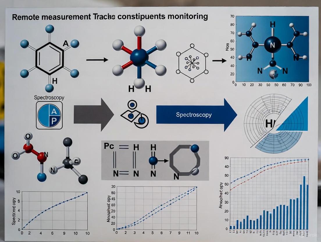
The accurate remote measurement of trace atmospheric constituents is a cornerstone of modern environmental research, directly impacting our understanding of climate change, air quality, and public health. This document provides detailed application notes and protocols for monitoring five key target analytes: ozone (O₃), nitrogen dioxide (NO₂), formaldehyde (HCHO), methane (CH₄), and aerosols. The techniques discussed herein, including hyperspectral imaging, multi-spectral satellite analysis, and ground-based in-situ quality control, are framed within the broader thesis that advances in remote sensing technology and data analytics are revolutionizing our ability to quantify and monitor atmospheric composition with unprecedented spatial and temporal resolution. The following sections summarize the core measurement principles, present quantitative data on emissions and performance, and outline standardized protocols for researchers and scientists.
Table 1: Key Target Analytes and Primary Remote Sensing Techniques
| Target Analyte | Primary Measurement Techniques | Key Spectral Regions | Major Impact/Concern |
|---|---|---|---|
| Nitrogen Dioxide (NO₂) | Fast-Hyperspectral Imaging, DOAS, TROPOMI [21] | UV-Visible (405, 470 nm) [21] | Air pollution, acid rain, respiratory issues |
| Sulfur Dioxide (SO₂) | Fast-Hyperspectral Imaging, DOAS, TROPOMI [21] | UV (310, 330 nm) [21] | Air pollution, acid rain |
| Methane (CH₄) | Multi-spectral Satellites (Sentinel-2), TROPOMI, Analytical Inversion [22] [23] | Short-Wave Infrared (SWIR) [22] | Potent greenhouse gas, climate forcing |
| Formaldehyde (HCHO) | Fluorescence, UV Spectrophotometry, DNPH Derivatization [24] | UV Fluorescence [24] | Carcinogen, indoor air quality, secondary pollutant |
| Aerosols | Multi-angle Polarimetry, Lidar, MODIS, MISR [25] | Multi-wavelength Visible to SWIR [25] | Climate forcing, air quality, human health |
Quantitative Data on Emissions and Detection
Recent studies leveraging satellite data have provided critical quantitative insights into the emissions of key atmospheric pollutants, particularly methane and nitrogen oxides. The data presented in the tables below offer a snapshot of current emission levels and the performance of state-of-the-art detection technologies.
Table 2: Urban Methane Emissions in North America from TROPOMI Data (2021) [23]
| City | Average Total Emission (Gg a⁻¹) | Scale Factor (Posterior/Prior) | Implication |
|---|---|---|---|
| Houston | 650.16 | 1.3 - 6.2 | Significant prior underestimation |
| Mexico City | 280.81 | 0.8 - 2.5 | Likely prior underestimation |
| Toronto | 230.52 | 0.9 - 3.0 | Likely prior underestimation |
| Los Angeles | 207.03 | 0.7 - 2.0 | Mixed agreement with prior |
| New York | 144.38 | 0.22 - 0.9 | Prior overestimation in some areas |
| Montreal | 111.54 | 0.5 - 1.5 | Reasonable prior agreement |
Table 3: Performance Comparison of Methane Detection Methods in Satellite Data
| Detection Method | Spectral Resolution | Spatial Resolution | Approx. Detection Limit | Key Advantage |
|---|---|---|---|---|
| Vision Transformer (Sentinel-2) [22] | Multi-spectral (~13 bands) | 20 m | 200-300 kg CH₄ h⁻¹ | High spatial/temporal resolution, global coverage |
| Hyperspectral Satellites (e.g., PRISMA) [22] | High (Hundreds of bands) | ~30 m | Low (precise quantification) | High spectral resolution for precise quantification |
| Sentinel-5P (TROPOMI) [23] | High | 5.5x7 km² | Regional scale | Daily global coverage, excellent for regional inversions |
| State-of-the-Art (MBMP) [22] | Multi-spectral | 20 m | 2-3 tons/h (deserts) | Baseline for performance comparison |
Detailed Experimental Protocols
Protocol: Fast-Hyperspectral Imaging for NO₂ and SO₂ Emission Quantification from Marine Vessels
This protocol describes the procedure for quantifying nitrogen dioxide (NO₂) and sulfur dioxide (SO₂) emissions from ship plumes using a custom fast-hyperspectral imaging remote sensing system [21].
1. Principle: The technique measures the differential slant column densities (DSCDs) of NO₂ and SO₂ by analyzing solar backscatter spectra in the UV and visible ranges. The absorption features of these gases are identified using the Differential Optical Absorption Spectroscopy (DOAS) method. A key innovation is the use of O₄ variation to categorize plumes as aerosol-present or aerosol-absent, which dictates the appropriate air mass factor (AMF) calculation scheme for converting DSCDs to vertical column densities (VCDs) [21].
2. Equipment and Reagents:
- Hyperspectral Imaging System: Comprising a hyperspectral camera, a visible camera, and a multiwavelength filter system on a UV camera, all co-axially designed.
- Spectrometer: A unit housed within a high-precision temperature control system (20 °C ± 0.5 °C) to reduce spectral noise.
- 2D Scanning System: An elevation and azimuth motor system to control the telescope's movement.
- Industrial Control Machine (IPC): Runs upper computer software for instrument control, data acquisition, and spectral analysis [21].
3. Procedure:
- Step 1: System Setup and Calibration. Deploy the instrument with a clear view of the target area (e.g., a shipping lane). Before measurements, conduct two zenith measurements to serve as reference spectra for the entire observation period. Verify the field of view (FOV) of the hyperspectral camera.
- Step 2: "S"-Shape Scanning. Initiate an automated "S"-shaped scanning trajectory using the 2D scanning system to cover the preset imaging area. The integration time for a single spectrum is typically 3 seconds. A complete scan of a vessel plume should take less than 4 minutes.
- Step 3: Multi-wavelength Filter Imaging. Simultaneously, use the multi-channel UV camera system to capture images through specific filter pairs: center wavelengths at 310/330 nm for SO₂ and 405/470 nm for NO₂. This aids in precise identification of the plume outline and internal trace gas distribution.
- Step 4: Data Processing - DSCD Retrieval. Process the collected solar scattering spectra using a DOAS-based algorithm to retrieve the DSCDs of NO₂ and SO₂.
- Step 5: Data Processing - Aerosol Categorization and AMF Calculation. Analyze the variation of O₄ DSCDs at a fixed elevation angle across different azimuth angles passing through the plume.
- If the standard deviation of O₄ DSCDs is <20%, categorize the plume as aerosol-absent. Retrieve aerosol vertical profiles from different azimuths and input them as constraints into a radiative transfer model (RTM) to calculate AMFs.
- If the standard deviation is ≥20%, categorize the plume as aerosol-present. The stereoscopic distribution of aerosols within the plume must be simulated and reconstructed using a 3D-RTM to derive accurate AMFs.
- Step 6: Quantification. Calculate the VCD of the target gas by dividing the DSCD by the appropriate AMF. Emission rates can be further derived using wind speed data and the cross-sectional extent of the plume [21].
Figure 1: Workflow for hyperspectral imaging of NO₂ and SO₂ from ship plumes, highlighting the critical decision point for aerosol-influenced air mass factor calculation [21].
Protocol: Automated Methane Point Source Detection using Sentinel-2 and a Vision Transformer
This protocol outlines the use of a deep learning model, specifically a Vision Transformer, to automatically detect methane point sources in multi-spectral satellite imagery from the Sentinel-2 constellation [22].
1. Principle: The model overcomes the inherent trade-off in multi-spectral satellites (high spatial resolution but low spectral information) by learning to recognize the subtle spectral signatures of methane in Sentinel-2's band 12 (SWIR) amidst noise. It uses a sequence-to-sequence prediction on a U-net architecture with a transformer encoder, taking two consecutive images as input to identify transient methane signals [22].
2. Equipment and Data:
- Sentinel-2 L1C Data: Top-of-Atmosphere reflectance data from Sentinel-2A and 2B satellites.
- Computing Infrastructure: GPU-accelerated computing environment capable of handling deep learning model training and inference on large datasets.
- Software: Python with deep learning frameworks (e.g., PyTorch, TensorFlow).
3. Procedure:
- Step 1: Data Collection and Pre-processing. Gather a large database of pairs of Sentinel-2 tiles from two consecutive times with minimal cloud cover (<25%). The data should be cut into 2.5 × 2.5 km² scenes and all input bands resampled to a uniform 20 m resolution.
- Step 2: Generation of Synthetic Training Data.
- Generate thousands of Gaussian plumes with varying emission rates and wind velocities.
- Add auto-correlated atmospheric noise to mimic turbulence.
- Embed these synthetic methane plumes into randomly selected real Sentinel-2 scenes using the Beer-Lambert law. This creates a large, diverse training dataset where the "ground truth" location of the plume is known.
- Step 3: Model Training. Train the Vision Transformer U-net model. The input is a stack of 10 spectral bands (B1, B2, B3, B4, B5, B8, B8A, B9, B11, B12) from both time steps (t-1 and t). The model's task is to classify the set of pixels corresponding to the embedded synthetic methane plume at time t.
- Step 4: Model Validation and Testing. Evaluate the model's performance on a held-out test set using metrics like F1-score and compare its performance against state-of-the-art methods like the normalized Multi-band multi-pass (MBMP) method. The model can reliably detect plumes with a signal-to-noise ratio (SNR) as low as 5%, an order of magnitude improvement over the previous method [22].
- Step 5: Application to Real-World Data. Deploy the trained model to analyze new, unseen Sentinel-2 data for automatic detection of methane point sources, enabling global monitoring every 2-5 days.
Protocol: Quality Control of In-Situ Atmospheric Composition Measurements
This protocol describes the use of the GAW-QC interactive dashboard for the quality control (QC) of near-realtime and historical in-situ measurements of trace gases like CH₄, CO, and CO₂ [6].
1. Principle: The dashboard combines three distinct anomaly detection algorithms to flag unreliable data points in hourly time series data from monitoring stations. It is intended as guidance for expert decision-making by station operators [6].
2. Equipment and Data:
- In-Situ Data: Hourly resolution data of target gases (e.g., CH₄, CO, CO₂) from monitoring stations.
- GAW-QC Dashboard: A web-based application implemented in Python using the Dash framework.
- Supporting Data: CAMS global atmospheric composition forecasts for independent comparison.
3. Procedure:
- Step 1: Data Input. Supply the dashboard with the station's hourly time series data for the target gas.
- Step 2: Anomaly Detection Execution. The dashboard runs three algorithms in parallel:
- Subsequence LOF: An unsupervised algorithm that identifies anomalous sequences of measurements on a scale of a few hours, effective for isolated outliers and changes in data variability.
- CAMS-ML Forecasts: A machine learning model uses CAMS numerical forecasts to predict expected concentrations at the station location. Significant deviations between measurements and predictions can indicate systematic biases or instrument drift.
- SARIMA Model: A Seasonal Autoregressive Integrated Moving Average model predicts monthly mean values based on the station's own historical data, highlighting outliers at a longer time scale.
- Step 3: Results Visualization. Review the dashboard's interactive interface, which displays the measurement time series overlaid with anomaly flags from the three methods.
- Step 4: Expert Review and Flagging. The station operator, using their local knowledge and the dashboard's guidance, makes the final decision on whether to flag data points as unreliable.
The Scientist's Toolkit: Essential Research Reagents & Materials
Table 4: Key Research Reagent Solutions and Materials for Atmospheric Monitoring
| Item / Solution | Function / Application | Example Context |
|---|---|---|
| DNPH (2,4-dinitrophenylhydrazine) | Derivatization agent for formaldehyde; reacts to form UV-emitting hydrazone for HPLC analysis [24]. | Passive and active sampling in indoor air quality surveys [24]. |
| High-Precision Temp Control System | Maintains spectrometer temperature (e.g., 20°C ±0.5°C) to minimize spectral noise and drift [21]. | Fast-hyperspectral imaging for NO₂/SO₂ [21]. |
| Multi-Wavelength Filters | Isolate specific absorption bands for target gases (e.g., 310/330 nm for SO₂) to improve plume visibility and specificity [21]. | UV camera system in hyperspectral imaging [21]. |
| Synthetic Training Data (Gaussian Plumes) | Used to train deep learning models to recognize gas plumes in satellite data where real labeled data is scarce [22]. | Vision Transformer for methane detection in Sentinel-2 imagery [22]. |
| CAMS Global Forecasts | Provides independent, gridded data of atmospheric composition for comparison with in-situ measurements to identify anomalies [6]. | Quality control of in-situ CH₄, CO, and CO₂ measurements [6]. |
Figure 2: Logical relationships between key remote sensing technologies and their primary applications in atmospheric constituent monitoring [21] [22] [6].
The targeted monitoring of these key analytes is critical for addressing pressing global challenges. Methane emissions, with a radiative forcing impact accounting for approximately one-third of warming to date, are a major short-term climate forcer [22]. Quantifying urban emissions, as shown in Table 2, is essential for verifying bottom-up inventories and guiding mitigation actions [23]. Nitrogen Dioxide and Sulfur Dioxide from sources like marine vessels significantly impact coastal air quality and contribute to acid rain [21]. Formaldehyde, a carcinogen, poses direct health risks, particularly in indoor environments, and can also be formed as a secondary pollutant [24]. Finally, aerosols exert a complex influence on the Earth's radiative balance, affect cloud formation and precipitation patterns, and have significant consequences for public health [25].
The protocols and technologies detailed herein—from the high spatiotemporal resolution of fast-hyperspectral imaging to the global, automated detection capabilities of AI-powered satellite analysis—represent the forefront of remote measurement techniques. The integration of these tools, supported by robust quality control frameworks, provides researchers and policymakers with the data necessary to understand, manage, and mitigate the impacts of these critical atmospheric constituents.
Atmospheric Chemistry and Transport Processes Affecting Measurement
Understanding atmospheric chemistry and transport processes is fundamental to the accurate remote measurement of trace atmospheric constituents. These processes control the distribution, transformation, and ultimate fate of gases and aerosols, directly influencing the signals detected by remote sensing instruments. This document provides application notes and detailed protocols for researchers and scientists engaged in monitoring research, with a specific focus on the context of measuring species relevant to environmental and climate studies. The accurate interpretation of remote sensing data, whether from satellite, aircraft, or ground-based platforms, requires a robust understanding of the atmospheric processes that modify concentration profiles between the source and the sensor.
Experimental Protocols for Model Validation Using Airborne Measurements
The following protocol outlines a methodology for evaluating the performance of atmospheric weather and chemical transport models against high-resolution in-situ measurements, a critical step in validating remote sensing data products.
Equipment and Measurement Platform
- Research Aircraft: Utilize instrumented aircraft such as an ATR42 or Cessna, equipped with in-situ gas analyzers (e.g., Picarro CRDS analyzers for CH4/CO2) calibrated to the WMO scale [26].
- Weather Balloons: Deploy CNES Light Inflatable Balloons (BLD) and Zero Pressure Difference (ZPD) balloons capable of reaching altitudes of 30 km or more [26].
- Instrumentation:
- Meteomodem M20 Radiosondes: For measuring temperature, humidity, pressure, and wind components during ascent and descent [26].
- AirCore Sampler: A coated stainless steel tube for collecting atmospheric air samples across a vertical profile from ~0–30 km for subsequent analysis of trace gas concentrations [26].
Field Campaign Execution
- Spatio-Temporal Design: Conduct measurements over multiple days (e.g., a 6-14 day campaign) to capture diurnal and synoptic variability. The MAGIC2021 campaign near Kiruna, Sweden (67° N) serves as a model [26].
- Profile Measurements: Execute coordinated flights and balloon launches to capture high-resolution vertical profiles of meteorological variables (T, P, RH, wind) and trace gas mixing ratios (e.g., CH4) from the surface to the lower stratosphere [26].
- Data Harmonization: Perform wing-by-wing inter-comparison flights and calibrate all analyzers using common gas standards to ensure data consistency across different platforms and instruments [26].
Model Comparison and Analysis
- Model Selection: Compare observations against a suite of models, which may include:
- Global Reanalysis: ECMWF ERA5 for meteorological variables [26].
- Regional Models: Weather Research and Forecasting (WRF) model and WRF-Chem for higher-resolution local dynamics and chemistry [26].
- Inversion-Optimized Models: Models like CAMS inversion products or PYVAR-LMDz-SACS ensemble inversions that adjust emissions to match observational constraints [26].
- Bias Assessment: Analyze model biases across different atmospheric layers, particularly in the planetary boundary layer (where emission uncertainties and turbulent transport dominate) and the stratosphere (where chemical loss and vertical resolution are critical) [26].
- Performance Metrics: Evaluate models based on their ability to replicate the observed vertical gradients and absolute mixing ratios, identifying potential overestimations in wetland emissions or inaccuracies in stratospheric transport [26].
The Scientist's Toolkit: Key Reagents and Research Solutions
The table below details essential materials, instruments, and computational tools used in atmospheric remote sensing and model validation studies.
Table 1: Key Research Reagent Solutions and Essential Materials for Atmospheric Monitoring
| Item Name | Function/Application |
|---|---|
| Passive Solar Remote Sensing Spectrometers (e.g., TROPOMI, GOME, SCIAMACHY, GEMS) | Nadir-viewing instruments on satellite platforms that use sunlight to measure total atmospheric columns of trace gases (e.g., O3, NO2, HCHO) via Differential Optical Absorption Spectroscopy (DOAS) [27]. |
| AirCore Atmospheric Sampler | Provides vertical profiles of trace gases (e.g., CH4, CO2) from the surface to the stratosphere, serving as a high-accuracy validation dataset for satellite retrievals and models [26]. |
| Fourier Transform Spectrometers (FTS) (e.g., ACE-FTS, MIPAS) | Limb-sounding or solar occultation instruments that provide high-resolution infrared spectra for identifying and quantifying a wide range of trace constituents in the upper troposphere and stratosphere [28] [29]. |
| Inversion-Optimized Flux Models (e.g., PYVAR-LMDz-SACS) | Atmospheric inversion systems that adjust a priori emission estimates (e.g., for wetlands) to better match atmospheric concentration observations, reducing flux uncertainties [26]. |
| Chemical Transport Models (CTMs) (e.g., WRF-Chem) | Regional or global models that simulate the emission, chemical transformation, and transport of atmospheric species; used for interpreting measurements and forecasting atmospheric composition [26]. |
| Calibration Gases (WMO Scale) | High-precision reference gases used to calibrate in-situ analyzers (e.g., Picarro), ensuring data is directly comparable to global monitoring networks like those operated by ICOS [26]. |
Data Presentation and Results
The evaluation of models against observational data yields critical quantitative insights. The following tables summarize typical findings regarding model performance and the capabilities of different measurement techniques.
Table 2: Summary of Model Performance in Simulating CH4 Profiles at High Latitudes (based on MAGIC2021 campaign data)
| Model / Product | Key Strengths | Identified Biases / Limitations |
|---|---|---|
| ERA5 Reanalysis (ECMWF) | Better overall agreement with observed meteorological variables compared to regional meso-scale models [26]. | --- |
| WRF Model | Provides valuable high-resolution insights into local atmospheric dynamics [26]. | Shows discrepancies in meteorological variables compared to ERA5 [26]. |
| Inversion-Optimized Models (e.g., CAMS, PYVAR-LMDz-SACS) | Best overall performance in simulating CH4 mixing ratios, particularly when constrained by surface measurements [26]. | --- |
| WRF-Chem Regional Simulations | --- | Positive bias in CH4 mixing ratios within the boundary layer, suggesting an overestimation of emissions from wetland models [26]. |
| All Chemistry-Transport Models | Models with higher vertical resolution show improved representation of vertical CH4 profiles in the upper atmospheric layers [26]. | Exhibit a consistent positive bias in the stratosphere [26]. |
Table 3: Techniques for Remote Sensing of Atmospheric Trace Constituents
| Technique | Platform Example | Measured Species | Technical Principle |
|---|---|---|---|
| Differential Optical Absorption Spectroscopy (DOAS) | TROPOMI (S5P), GEMS, AIRMAP (Aircraft) [27] | O3, NO2, BrO, OClO, IO, HCHO, CHO.CHO, H2O (in UV/Vis) [27] | Measures unique absorption fingerprints of gas molecules in ultraviolet and visible solar backscatter spectra. |
| Nadir Thermal Emission Spectroscopy | IASI [30] | Global radiometry for temperature and humidity profiles [30] | Measures the infrared thermal emission from the Earth-atmosphere system. |
| Fourier Transform Spectrometry (FTS) | ACE-FTS, MIPAS-B (Balloon) [28] [29] | Wide range of species including C2H4, HFC-23, HFC-125, SO2, aerosols [29] | Uses an interferometer to capture high-resolution mid-infrared spectra for precise species identification and quantification. |
| Gas Chromatography-Mass Spectrometry (GC-MS) | Laboratory analysis of AirCore and flask samples [31] | Pesticides, pharmaceuticals, complex organic mixtures [31] | Separates complex mixtures (GC) and provides definitive identification and quantification via mass spectral fragmentation (MS). |
Workflow Visualization
The following diagram illustrates the integrated workflow for validating remote sensing data and atmospheric models using a multi-platform campaign approach.
Workflow for Validating Remote Sensing Data and Models
Advanced Monitoring Platforms and Analytical Techniques in Practice
Satellite-based remote sensing has revolutionized the capacity to monitor trace atmospheric constituents on a global scale. The two primary orbital configurations used for atmospheric observation—geostationary and polar-orbiting—offer complementary capabilities that form the backbone of modern environmental monitoring systems. Geostationary satellites maintain a fixed position approximately 36,000 km above the equator, providing constant observation over a specific hemisphere [32]. This continuous vantage point enables high-temporal resolution monitoring, making them ideal for tracking rapidly evolving atmospheric phenomena. In contrast, polar-orbiting satellites operate at lower altitudes (typically 800-850 km) in a sun-synchronous orbit, passing over the polar regions multiple times daily [33]. Their closer proximity to Earth and global coverage pattern provide higher spatial resolution data, albeit with less frequent revisits over any given location.
The synergy between these platforms is critical for advancing understanding of atmospheric chemistry, transport mechanisms, and the impacts of trace gases and aerosols on climate, weather, and public health. This document details the specific applications, experimental protocols, and data utilization methods for both geostationary and polar-orbiting satellite systems within the context of remote measurement techniques for trace atmospheric constituents.
Platform Comparison and Operational Characteristics
The distinct orbital mechanics of geostationary and polar-orbiting satellites directly define their observational strengths and limitations. The following table summarizes their key characteristics and operational parameters.
Table 1: Comparative Analysis of Geostationary and Polar-Orbiting Satellite Platforms
| Characteristic | Geostationary Satellites | Polar-Orbiting Satellites |
|---|---|---|
| Orbital Altitude | ~36,000 km [32] | ~823-850 km [33] |
| Orbital Period | 24 hours (synchronized with Earth's rotation) | ~100 minutes [32] |
| Spatial Resolution | Lower due to high altitude [34] | Higher due to lower altitude [34] |
| Temporal Resolution | Very high (minutes to hours) [34] | Lower (once to twice daily per location) |
| Typical Coverage | Fixed disk (e.g., full hemisphere) [32] | Global, pole-to-pole [33] [32] |
| Polar Region View | Poor, with significant parallax [34] [32] | Excellent, with multiple daily passes [32] |
| Primary Application Strengths | Nowcasting, diurnal cycle studies, severe weather tracking [34] [35] | Numerical weather prediction, global climate monitoring, air quality mapping [33] [36] |
This complementary relationship is operationalized in systems like Europe's dual-orbit strategy, which employs the geostationary Meteosat series alongside the polar-orbiting Metop satellites to provide a complete picture of atmospheric dynamics [32].
Application Notes: Monitoring of Trace Atmospheric Constituents
Capabilities of Geostationary Platforms
The high temporal resolution of geostationary satellites is uniquely suited for monitoring atmospheric constituents with significant diurnal variability. A prime example is the monitoring of ozone (O₃), a potent greenhouse gas and air pollutant whose formation is driven by photochemical reactions that fluctuate throughout the day. Traditional polar-orbiting satellites provide only a single daily snapshot, often missing the peak concentration periods. The next-generation Geostationary Environment Monitoring Spectrometer (GEMS), with its ultraviolet capabilities and hourly measurements, has demonstrated a profound improvement in accuracy. It achieves a high coefficient of determination (R² = 0.94) for retrieving hourly O₃ concentrations, leading to a more precise calculation of the Daily Maximum 8-hour Average (MDA8), a key metric for health impact assessments [35]. This technological advancement revealed that previous estimates from polar-orbiters likely overestimated O₃-related health risks by approximately 30%, particularly in semi-urban and rural areas [35]. This capability is critical for regulatory compliance and designing effective control strategies.
Capabilities of Polar-Orbiting Platforms
Polar-orbiting satellites provide essential global, high-resolution data for a comprehensive suite of atmospheric variables. The EUMETSAT Polar System – Second Generation (EPS-SG), featuring the Metop-SG satellites, exemplifies this capability. The system employs a pair of satellites (SGA and SGB) with complementary instrument suites [33]. Metop-SGA carries atmospheric sounding and imaging instruments for optical, infrared, and microwave observations, providing critical data on temperature, moisture, and aerosols [33]. A cornerstone of its payload is the Copernicus Sentinel-5 spectrometer, which is dedicated to observing trace gases like ozone, nitrogen dioxide, sulphur dioxide, carbon monoxide, and methane, as well as aerosols [33] [32]. Metop-SGB hosts additional technologies, including microwave and scatterometer instruments, that deliver observations of precipitation, ice clouds, and other parameters [33]. This global coverage is indispensable for numerical weather prediction, climate monitoring, and tracking long-range transport of pollution [33] [36].
Integrated Applications for Public Health and Climate
Satellite remote sensing bridges a critical gap in ground-based monitoring networks, which are often unevenly distributed and lack sufficient spatial coverage [37]. By providing continuous spatial observations, satellites enable global air quality surveillance and exposure assessment. Data from polar-orbiting instruments like IASI and GOME-2 on legacy Metop satellites, and the upcoming Sentinel-5 on Metop-SG, form critical inputs for monitoring air quality and climate-forcing agents such as methane [36] [38]. Methane, with a global warming potential over 80 times that of CO₂ over 20 years, is a prime target for satellite monitoring. New satellite constellations, including commercial nanosatellites, are being developed to detect methane emissions with high precision, identifying sources as small as 100 kilograms per hour [38]. This data is vital for verifying national emission inventories and guiding mitigation efforts under initiatives like the Global Methane Pledge [38].
Experimental Protocols and Workflows
Protocol 1: Retrieval of Hourly Ground-Level Ozone using Geostationary Satellite Data
This protocol details the methodology for leveraging the high temporal resolution of geostationary satellites, such as GEMS, to accurately capture the diurnal variation of ground-level ozone, a significant improvement over polar-orbiting methods [35].
- Objective: To retrieve accurate hourly ground-level ozone concentrations and calculate the Daily Maximum 8-hour Average (MDA8-O₃) for health exposure assessments.
- Principle: Utilizes the geostationary satellite's hourly measurements of ozone precursors (e.g., nitrogen dioxide) and ultraviolet radiation to represent the photochemistry driving ozone formation throughout the day.
- Materials and Instruments:
- Geostationary Satellite Data: Hourly Level-2 data from GEMS or an equivalent platform, including column density of NO₂ and UV irradiance measurements.
- Ancillary Meteorological Data: Reanalysis or model data for relative humidity, temperature, and boundary layer height.
- Ground-Truthing Data: Hourly in-situ ozone measurements from monitoring stations for model training and validation.
- Computational Environment: Machine learning software (e.g., Python with Scikit-learn, TensorFlow, or R) and high-performance computing resources.
- Procedure:
- Data Collection and Collocation: For a defined study period and region, collocate hourly GEMS observations of NO₂ and UV data with corresponding ground-based ozone measurements and meteorological parameters. Ensure spatial and temporal matching.
- Model Training: Train a time-specific machine learning model (e.g., a separate model for each hour of the day) to establish the non-linear relationship between the satellite-observed parameters (precursors, UV) and the ground-level ozone concentration.
- Spatial Prediction: Apply the trained models to the full, gridded GEMS dataset to generate maps of estimated hourly ground-level ozone concentrations across the entire domain covered by the satellite.
- MDA8-O₃ Calculation: For each grid cell, process the time series of predicted hourly ozone concentrations to derive the MDA8-O₃ value for each day.
- Validation: Validate the final MDA8-O₃ estimates against held-out ground station data, reporting performance metrics such as R² and Root Mean Squared Error (RMSE).
The following workflow diagram illustrates this multi-stage process:
Protocol 2: Global Trace Gas Mapping with Polar-Orbiting Satellites
This protocol describes the end-to-end process for generating global maps of trace gases and aerosols using instruments aboard polar-orbiting satellites like the Sentinel-5 spectrometer on Metop-SG.
- Objective: To produce global, spatially-continuous maps of atmospheric trace constituents (e.g., NO₂, SO₂, O₃, CH₄, aerosols) for climate and air quality applications.
- Principle: Measures the absorption and scattering of solar radiation at specific wavelengths as it passes through the atmosphere to retrieve the total vertical column density of target gases.
- Materials and Instruments:
- Satellite Data: Level-1 data from a polar-orbiting spectrometer (e.g., Sentinel-5, TROPOMI).
- Radiative Transfer Model: Software such as SCIATRAN or VLIDORT to simulate light propagation through the atmosphere.
- Auxiliary Data: Digital Elevation Models (DEMs) and a priori information on atmospheric profiles.
- Validation Data: Ground-based measurements from networks like Pandora or AERONET, and aircraft campaign data.
- Procedure:
- Level-1 Data Acquisition: Download the top-of-atmosphere radiance measurements from the satellite data provider for the target area and time period.
- Pre-processing: Apply corrections for instrument-specific effects, including radiometric calibration and geo-referencing.
- Forward Modeling: Use the radiative transfer model to simulate the radiance that the satellite would measure for a given state of the atmosphere and surface.
- Inversion: Retrieve the target gas column density by iteratively adjusting the atmospheric state in the forward model until the simulated radiance matches the actual satellite measurement. This often involves a dedicated retrieval algorithm (e.g., the Differential Optical Absorption Spectroscopy - DOAS - technique).
- Post-processing: Filter the results based on quality flags (e.g., cloud cover, snow/ice, solar zenith angle) and apply any necessary bias corrections.
- Validation: Compare the satellite-derived data products with independent ground-based or airborne measurements to quantify accuracy and precision.
The logical flow of this retrieval process is shown below:
The Scientist's Toolkit: Essential Research Reagents and Materials
In the context of satellite remote sensing for atmospheric constituents, "research reagents" refer to the essential datasets, algorithms, and software tools required to convert raw satellite measurements into scientifically valuable data products.
Table 2: Essential Research Reagents for Satellite Atmospheric Monitoring
| Reagent / Material | Type | Function / Application |
|---|---|---|
| Level-1 Top-of-Atmosphere Radiance | Primary Satellite Data | The fundamental measurement from the satellite instrument; the starting point for all retrievals. |
| Radiative Transfer Model (RTM) | Algorithm / Software | Simulates the passage of radiation through the atmosphere; core component of the retrieval algorithm to relate atmospheric state to measured radiance. |
| A Priori Atmospheric Profiles | Ancillary Data | Provides initial estimates of atmospheric conditions (e.g., temperature, pressure, gas profiles) to constrain the retrieval inversion, which is an ill-posed problem. |
| Machine Learning Models (e.g., Random Forest, Neural Networks) | Algorithm | Used to establish complex, non-linear relationships between satellite measurements and ground-level concentrations, particularly for geostationary data analysis. |
| Ground-Based Validation Data | Validation Data | In-situ measurements from monitoring stations; serve as "ground truth" to validate and quantify the uncertainty of satellite-derived products. |
| Digital Elevation Model (DEM) | Ancillary Data | Provides information on surface elevation and terrain, which is critical for accurate radiative transfer modeling and geo-location. |
| Geostationary Satellite Data (e.g., GEMS) | Primary Satellite Data | Provides high-temporal-resolution data on trace gases and precursors, enabling study of diurnal cycles and photochemistry. |
| Polar-Orbiting Satellite Data (e.g., Sentinel-5) | Primary Satellite Data | Provides high-spatial-resolution global data on a wide range of trace gases and aerosols for mapping and long-term trend analysis. |
The synergistic use of geostationary and polar-orbiting satellite platforms provides an unparalleled capability for monitoring Earth's atmospheric composition. While geostationary satellites excel at capturing the dynamics of diurnal processes critical for understanding photochemical pollution and nowcasting, polar-orbiting satellites offer the high-resolution global mapping essential for numerical weather prediction, climate monitoring, and verifying emission inventories. The ongoing development of new satellite systems, such as the Metop-SG series and advanced geostationary sensors like GEMS, along with sophisticated retrieval algorithms and machine learning techniques, continues to enhance the accuracy, resolution, and utility of atmospheric data. This integrated observational capability is fundamental for addressing pressing global challenges related to air quality, public health, and climate change.
Remote sensing technologies are indispensable for monitoring trace atmospheric constituents, providing critical data on their distribution, concentration, and impact on environmental processes. These instruments, deployed on both ground-based platforms and aircraft, enable scientists to observe atmospheric chemistry and dynamics at various scales without direct contact. Lidar systems use laser pulses to profile aerosols, clouds, and gases, while spectrometers identify and quantify molecular species through their unique spectral fingerprints. Radiometers measure the intensity of electromagnetic radiation, providing data on atmospheric properties and surface characteristics. This article details the application of these technologies within a research framework focused on trace gas and aerosol monitoring, providing structured data comparisons, experimental protocols, and essential resource guides for researchers and scientists.
Core Technologies and Instrumentation
The selection of appropriate remote sensing technology is guided by the target analyte, required spatial and temporal resolution, and the platform constraints. The table below summarizes the primary instruments used in atmospheric monitoring research.
Table 1: Key Remote Sensing Instruments for Atmospheric Constituents Monitoring
| Instrument Type | Primary Function | Typical Measured Constituents | Common Platforms | Key Characteristics |
|---|---|---|---|---|
| Lidar | Profiles atmospheric properties using laser pulses. | Aerosols, clouds, water vapor, methane, ozone [39] [40]. | Aircraft, Ground Stations | Active sensing; provides high vertical resolution; can penetrate vegetation [41]. |
| Spectrometer | Identifies and quantifies gases by analyzing absorption spectra. | Carbon dioxide (XCO₂), Solar-Induced Fluorescence (SIF), ozone-depleting substances [40] [42]. | Satellites (e.g., OCO-2, OCO-3), Aircraft, Ground Stations | Passive and active variants; high spectral resolution for discerning specific gases. |
| Microwave Radiometer | Measures microwave emissions to derive atmospheric and surface properties. | Water vapor, cloud liquid water, precipitation, sea-ice concentration [40]. | Satellites (e.g., with ATMS), Aircraft | Provides data in all weather conditions; sensitive to hydrometeors. |
Integrated sensor systems represent a significant advancement, combining the strengths of multiple instruments. For instance, modern airborne campaigns often deploy systems that tightly integrate lidar units with high-resolution digital cameras (RGB, NIR). This synergy allows for the simultaneous collection of 3D topographic data and high-resolution imagery, enhancing the interpretability of the laser data and enabling comprehensive environmental analysis [41]. Systems like the Leica CityMapper-2 and Vexcel Imaging's UltraCam Dragon 4.1 exemplify this approach, combining lidar with nadir and oblique cameras for optimal data collection in complex environments like urban areas [41].
Application in Contemporary Research
Recent field campaigns and research initiatives highlight the critical application of these technologies in addressing pressing environmental science questions.
Table 2: Select Recent Research Campaigns and Sensor Applications
| Campaign / Initiative | Primary Instruments | Target Constituents & Objectives | Key Findings & Outcomes |
|---|---|---|---|
| ARCSIX (Arctic Radiation-Cloud-Aerosol-Surface Interaction EXperiment) [40] | Airborne HALO Lidar. | Profiles of water vapor, methane, and aerosol/cloud optical properties. | Aims to quantify contributions to the Arctic summer surface radiation budget and sea ice melt. |
| PACE-PAX (Plankton, Aerosol, Cloud, ocean Ecosystem Postlaunch Airborne eXperiment) [40] | ER-2 Aircraft In-Situ Sensors (Meteorology/Navigation). | Validation and refinement of PACE satellite data products over coastal California. | Ensures accuracy and reliability of satellite-based ocean color, aerosol, and cloud data. |
| ALOFT (Airborne Lightning Observatory for FEGS and TGFs) [40] | Airborne Advanced Microwave Precipitation Radiometer (AMPR), Cloud Radar System (CRS). | Gamma-ray flashes in thunderstorms; cloud, precipitation, and water vapor properties. | Provides multi-frequency microwave imagery for deriving cloud and precipitation properties. |
| Student Airborne Research Program (SARP) - West [39] | Whole Air Sampling (canisters) followed by laboratory analysis (GC-MS). | Volatile Organic Compounds (VOCs) from dairies and wildfires; ozone production potential. | Identified methanol and ethanol as major VOC contributors to ozone formation in dairy regions [39]. |
| Copernicus Atmosphere Monitoring Service (CAMS) [42] | Satellite and Ground-Based Sensors (e.g., OMPS). | Antarctic ozone hole development and concentrations of ozone-depleting substances. | Tracked highly variable 2025 ozone hole, providing daily forecasts and analyses of ozone layer status [42]. |
Experimental Protocols and Methodologies
Protocol: Airborne Lidar Data Acquisition for Atmospheric Profiling
This protocol outlines the procedure for operating an integrated airborne lidar system, such as those used in NASA's ARCSIX campaign, to profile trace gases and aerosols [40] [41].
Workflow Diagram: Airborne Lidar Data Acquisition and Processing
1. Pre-Flight Planning:
- Objective Definition: Clearly define the target constituents (e.g., methane, aerosols) and the geographical area of interest.
- Flight Line Design: Plan parallel flight lines with sufficient side overlap (e.g., ≥20-50%) to ensure complete coverage and mitigate data gaps [41]. Consider atmospheric conditions and sun angle.
- Sensor Configuration: Set the laser pulse repetition rate (PRR), scan angle (FOV), and ensure tight integration and calibration of the GNSS, IMU, and laser scanner subsystems [41].
2. In-Flight Operation:
- System Power-On: Execute pre-defined calibration sequences for all sensors.
- Data Acquisition: During the flight, the system continuously operates:
- Laser Scanning: The scanner unit (e.g., using a rotating polygon mirror or Risley prism) deflects laser pulses across the flight path [41].
- Ranging: The ranging unit measures the time-of-flight of the laser pulses to calculate distances.
- Navigation: The GNSS receiver and IMU record the aircraft's precise position (latitude, longitude, altitude) and attitude (pitch, roll, yaw) at a high frequency [41].
- Data Logging: All data streams (laser returns, position, attitude) are synchronously logged with precise time stamps.
3. Post-Flight Data Processing:
- Data Transfer: Securely transfer raw data from the aircraft systems to a processing facility.
- Point Cloud Generation: Process the raw laser ranges with the navigation data to compute the 3D coordinates (X, Y, Z) for each laser return, creating a dense point cloud [41].
- Geolocation and Annotation: Assign geographic coordinates to each point. Annotate points with additional information, such as signal intensity or reflectance.
- Analysis: The processed data can be used to generate vertical profiles of aerosol backscatter or specific gas concentrations (e.g., methane columns from integrated path differential absorption lidar) [40].
Protocol: Whole Air Sampling for Volatile Organic Compound (VOC) Analysis
This protocol details the methodology for collecting and analyzing whole air samples to quantify VOCs, as practiced in the SARP West campaign [39].
Workflow Diagram: Whole Air Sampling and VOC Analysis
1. Sample Collection:
- Canister Preparation: Use electropolished stainless-steel canisters. Prior to deployment, clean and evacuate the canisters to a high vacuum to prevent contamination.
- Field Deployment: Deploy canisters at strategically chosen upwind and downwind sites to assess source impact and background concentrations [39].
- Sample Collection: Open the canister valve for a predetermined time or use a flow controller to fill the canister to ambient pressure. Document sample location, time, date, and meteorological conditions.
2. Laboratory Analysis:
- Gas Chromatography-Mass Spectrometry (GC-MS): Introduce an aliquot of the air sample into the GC-MS system.
- Separation: The GC column separates the complex mixture of VOCs based on their chemical properties and interaction with the column.
- Detection: The mass spectrometer ionizes the separated compounds and identifies them based on their unique mass-to-charge ratio (m/z) fragmentation patterns [39].
- Quantification: Concentrations of speciated VOCs (e.g., methanol, ethanol, alkanes, aromatics) are determined by comparing their signal response to calibrated standards [39].
3. Data Interpretation and Modeling:
- Source Apportionment: Compare concentrations between source (e.g., dairy farms) and downwind sites to determine enhancement levels [39].
- Ozone Production Potential (OPP) Calculation: Estimate the reactivity and contribution to ozone formation by multiplying the concentration of each VOC by its respective hydroxyl radical (OH) reaction rate constant [39].
- Dispersion Modeling: Use trajectory models like HYSPLIT to understand air mass transport and identify impacted communities [39].
The Scientist's Toolkit: Essential Research Reagents and Materials
Table 3: Key Research Reagent Solutions and Materials for Atmospheric Remote Sensing
| Item Name | Function / Application | Example Use-Case |
|---|---|---|
| Electropolished Stainless-Steel Canisters | Collection and storage of whole air samples for subsequent laboratory analysis of VOCs and other trace gases. | SARP West study on VOC emissions from dairies and wildfires [39]. |
| Calibrated Gas Standards | Quantification of target analytes during instrumental analysis; essential for generating calibration curves. | Used in GC-MS analysis of whole air samples to determine precise concentrations of methanol, ethanol, etc. [39]. |
| High-Purity Zero Air | A gas mixture free of the analytes of interest; used for instrument background correction and dilution of standards. | Flushing and blanking of analytical systems like GC-MS to ensure no contamination between samples. |
| Spectral Calibration Lamps | Sources of light with known, stable emission lines; used to validate and calibrate the wavelength accuracy of spectrometers. | Ensuring the spectral fidelity of instruments like the OCO-2 and OCO-3 for accurate XCO₂ retrievals [40]. |
| Neural Network Parameter Sets | Pre-trained algorithms that map physical oceanographic data to water mass age and anthropogenic carbon content. | Enabling rapid estimation of ocean Canth with the TRACEv1 software from simple input parameters [43]. |
Differential Optical Absorption Spectroscopy (DOAS) is a powerful analytical technique for the remote measurement of trace atmospheric constituents. This method leverages the unique absorption fingerprints of gaseous molecules in the ultraviolet (UV), visible (VIS), and near-infrared regions of the electromagnetic spectrum to identify and quantify their concentrations in the atmosphere [44]. Since its earliest reported use for monitoring NO₂ concentrations in 1973 [45], DOAS has evolved into a well-established method with applications spanning from industrial emission monitoring to global satellite-based atmospheric observation [13]. The technique's non-contact nature, ability to monitor multiple gases simultaneously, and capacity for path-integrated measurements make it particularly valuable for atmospheric research and environmental monitoring programs worldwide.
Core Principles of DOAS
The fundamental principle underlying DOAS is the Beer-Lambert absorption law, which describes the relationship between the amount of light absorbed and the concentration of absorbing molecules along the light path [44]. When light passes through a medium containing absorbing species, its intensity decreases proportionally to the concentration of these species and the path length.
The mathematical foundation of DOAS utilizes the differential absorption concept. The technique separates the measured absorption cross-section into two components: a slowly varying part (primarily due to Rayleigh and Mie scattering) and a rapidly varying part (due to specific molecular absorption features) [45]. By applying mathematical tools such as Fourier Transform filters to eliminate the slowly varying components, DOAS isolates the characteristic differential absorption structures unique to each molecule [45]. This differential approach significantly enhances the specificity and sensitivity of the measurements, allowing for precise quantification of trace gases even in complex atmospheric matrices.
Each gaseous molecule possesses a unique absorption fingerprint - characteristic wavelengths at which it absorbs light [44]. The DOAS method identifies gases by comparing measured differential absorption spectra with reference spectra of known gases, enabling both qualitative identification and quantitative analysis of multiple atmospheric constituents simultaneously.
Instrumentation and Research Toolkit
Essential DOAS System Components
A typical DOAS system consists of several key components that work together to acquire spectral data for atmospheric analysis [45] [44].
Table 1: Essential Components of a DOAS Instrumentation System
| System Component | Type/Examples | Key Function | Performance Considerations |
|---|---|---|---|
| Light Source | Xenon lamp [44], Deuterium (D₂) lamp [45], Sunlight [45] | Provides broadband light covering UV, visible, and/or IR regions | Spectral stability, intensity, and lifetime |
| Spectrometer | AvaSpec-ULS2048XL-EVO, AvaSpec-ULS2048x64-EVO [45] | Disperses light into constituent wavelengths for detection | Resolution, stray light rejection, signal-to-noise ratio |
| Detector | Back-thinned CCD, CMOS [45] | Converts spectral light into electrical signals | Sensitivity (especially in UV), dynamic range, dark noise |
| Optical Path | Retro-reflectors, telescope systems [45] | Defines measurement path through the atmosphere | Path length stability, alignment maintenance |
| Signal Processing | Fourier Transform filters [45] | Extracts differential absorption features from measured spectra | Algorithm efficiency, reference spectrum quality |
Key Research Reagent Solutions
While DOAS is primarily an optical technique without chemical reagents, its implementation relies on critical reference materials and computational resources.
Table 2: Essential Research Materials for DOAS Applications
| Resource Type | Specific Examples | Function in DOAS Research |
|---|---|---|
| Reference Spectra | Laboratory-measured cross-section spectra (NO₂, SO₂, HCHO, etc.) [46] | Enable quantitative analysis by providing standard absorption fingerprints for spectral fitting |
| Calibration Gases | Certified concentration standards in gas cells | Validate instrument performance and retrieval algorithms |
| Radiative Transfer Models | SCIATRAN, LIDORT | Simulate light path through the atmosphere for accurate column density determination |
| Spectral Analysis Software | DOASIS, QDOAS | Implement core retrieval algorithms and statistical analysis of differential absorption |
DOAS Application Methodologies
Active DOAS Systems for Emission Monitoring
Active DOAS systems employ artificial light sources for controlled measurement of gas concentrations, particularly useful for industrial emission monitoring [45].
Figure 1: Active DOAS System Configuration for Stack Emission Monitoring
Experimental Protocol - Continuous Emission Monitoring System (CEMS):
System Setup: Install a deuterium (D₂) lamp or xenon lamp light source on one side of the measurement area (e.g., smoke stack plume) [45]. Position a concave mirror on the opposite side to reflect light back to the collection system, or use a separate telescope system for single-ended operation.
Light Path Configuration: Align the system to establish a stable light path through the region of interest. For stack emissions, typical path lengths range from 2-20 meters depending on stack diameter and expected concentrations [45].
Reference Spectrum Acquisition: Collect a reference spectrum with the light path positioned to avoid the pollutant plume (when possible), or use a mathematically derived reference from spectral regions with minimal absorption by target gases.
Sample Measurement: Direct the light beam through the measurement path containing the analyte. For quantitative analysis, precisely determine the path length, as concentration calculations depend on this parameter.
Spectral Acquisition: Use a fiber-optic cable to direct the transmitted light to a spectrometer with appropriate spectral range and resolution [45]. For UV/VIS measurements of common pollutants (SO₂, NO₂), select a spectrometer covering 200-460 nm with resolution better than 0.5 nm.
Differential Processing: Apply the DOAS algorithm to the measured spectrum:
- Divide the sample spectrum by the reference spectrum
- Convert to absorbance units
- Apply high-pass filtering to separate broad spectral features from differential absorption structures
- Fit reference absorption cross-sections to the differential spectrum using least-squares algorithms
Concentration Retrieval: Calculate path-averaged concentrations using the differential optical density and known absorption cross-sections of the target molecules, applying the Beer-Lambert law in its differential form.
Passive DOAS Systems for Atmospheric Monitoring
Passive DOAS utilizes natural light sources (primarily sunlight) for atmospheric measurements, enabling both ground-based and satellite monitoring of trace gases [13].
Figure 2: Passive DOAS Configuration for Atmospheric Monitoring
Experimental Protocol - Multi-Axis (MAX-DOAS) Measurements:
Instrument Configuration: Deploy a spectrometer system with appropriate spectral range and resolution for target gases. For NO₂, SO₂, and HCHO measurements, the AvaSpec-ULS2048x64TEC-EVO spectrometer configured from 300 to 450 nm has been successfully employed [45]. Either 25μm slit (~0.25 nm resolution) or 50μm slit (~0.38 nm resolution) can be used depending on sensitivity requirements.
Pointing System Setup: Implement a telescope system capable of measuring scattered sunlight at multiple elevation angles (typically from 1° to 90°). Precise pointing accuracy is critical for consistent measurements.
Reference Spectrum Selection: Use solar spectra measured at high elevation angles (90°) as reference, where the atmospheric path is shortest, or utilize solar reference spectra from literature convolved to the instrument's spectral resolution.
Spectral Sequence Acquisition: Collect spectra sequentially at different elevation angles with identical integration times. Typical measurement sequences include 5-10 elevation angles with multiple measurements per angle to improve signal-to-noise ratio.
Differential Slant Column Retrieval: For each elevation angle, retrieve the differential slant column density (dSCD) - the integrated concentration along the light path - by applying DOAS fitting procedures to the measured spectra relative to the reference spectrum.
Profile Inversion: Apply radiative transfer modeling and inversion algorithms to convert the set of dSCDs at different elevation angles into vertical concentration profiles and vertical column densities of trace gases.
Validation: Compare retrieved vertical columns with complementary measurements such as satellite overpass data, in-situ instruments, or chemical transport models to validate measurement accuracy [13].
Advanced Applications in Atmospheric Research
Satellite-Based Atmospheric Composition Monitoring
The DOAS technique has been successfully implemented on satellite platforms for global monitoring of atmospheric trace constituents. Recent instruments include TROPOMI on the Copernicus Sentinel-5 Precursor and GEMS on the GEO-KOMPSAT-2B satellite [13]. These advanced systems retrieve total column amounts of key trace gases including ozone (O₃), nitrogen dioxide (NO₂), bromine monoxide (BrO), chlorine dioxide (OClO), formaldehyde (HCHO), glyoxal (CHO.CHO), and water vapor (H₂O) from UV and visible spectral ranges [13].
Satellite DOAS applications have revolutionized our ability to monitor global pollution transport, identify emission hotspots, and track long-term trends in atmospheric composition. For example, TROPOMI data has been used to validate urban emissions of NO₂ and measure methane (CH₄) and carbon dioxide (CO₂) columns, contributing essential data for climate change research [13].
Mobile Mapping of Trace Gas Distributions
Mobile DOAS systems installed on aircraft and ground vehicles provide high spatial resolution mapping of trace gas distributions. The AIRMAP and MAMAP instrument families have been developed to measure in the ultraviolet/visible and the near-infrared/shortwave-infrared regions, enabling determination of high spatial resolution trace column amounts [13]. These mobile applications are particularly valuable for quantifying emissions from area sources such as cities, agricultural regions, and industrial complexes that are difficult to characterize with stationary monitors.
Current Research Trends and Validation
Recent research presented at the International DOAS Workshop 2025 highlighted several emerging trends, including network development and harmonization across DOAS observations, validation and data-assimilation applications with DOAS observations, and advancements in DOAS spectral retrievals [47]. The integration of DOAS measurements with other observational techniques and models continues to enhance the value of these observations for understanding atmospheric processes and validating satellite data products.
Ongoing method development focuses on improving detection limits, expanding the range of measurable species, enhancing instrumental portability and autonomy, and developing more sophisticated retrieval algorithms that can better account for complex atmospheric scattering and absorption processes. These advancements ensure that DOAS remains at the forefront of atmospheric remote sensing techniques for trace gas monitoring.
Laser Spectrometers for High-Precision Trace Gas Detection
High-precision trace gas detection is fundamental to advancements in atmospheric science, climate research, and environmental monitoring. Laser absorption spectroscopy has emerged as a premier technique for quantifying atmospheric constituents, offering exceptional sensitivity, selectivity, and non-intrusive measurement capabilities [48] [49]. These techniques leverage the fundamental principle that gaseous molecules absorb light at specific, unique wavelengths, creating a spectroscopic fingerprint that allows for both identification and quantification [49]. The core relationship governing quantitative analysis is the Beer-Lambert law, which describes the attenuation of light as it passes through a gas sample: I(ν) = I₀(ν) × exp(-σ(ν) × L × C), where I(ν) is the transmitted intensity, I₀(ν) is the incident intensity, σ(ν) is the absorption cross-section, L is the optical path length, and C is the gas concentration [49].
Within the mid-infrared (MIR) spectral region (2.5–25 μm), molecules exhibit their strongest fundamental rovibrational absorption bands, providing a nearly universal and highly sensitive means for their detection [49]. This application note details the core methodologies, instrumental configurations, and experimental protocols for employing laser spectrometers in high-precision trace gas sensing, contextualized within remote measurement techniques for atmospheric constituent monitoring.
Technical Specifications of Laser Spectrometry Techniques
Various laser spectroscopic techniques have been developed to optimize sensitivity, selectivity, and practicality for trace gas detection. The choice of technique often involves a trade-off between these parameters, depending on the specific application requirements, such as necessary detection limits, sample volume availability, and whether field-based or laboratory-based measurements are needed.
Table 1: Comparison of Laser Spectrometry Techniques for Trace Gas Detection
| Technique | Principle of Operation | Typical Absorption Sensitivity | Key Advantages | Common Applications |
|---|---|---|---|---|
| Direct Absorption Spectroscopy (DAS) | Measures light attenuation directly according to Beer-Lambert law. | ~10⁻³ | Simple optical configuration; potential for absolute measurement. | Industrial process control; fundamental line strength measurements. |
| Wavelength Modulation Spectroscopy (WMS) | Modulates laser wavelength at high frequency; detects signal at a harmonic (e.g., 2f) using a lock-in amplifier. | ~10⁻⁵ | Reduces 1/f noise; robust against laser power fluctuations. | Continuous emission monitoring; atmospheric sensing in noisy environments. |
| Cavity Ring-Down Spectroscopy (CRDS) | Measures the decay rate of light trapped in a high-finesse optical cavity containing the sample. | ~10⁻⁷ – 10⁻⁹ | Very long effective path lengths; highly sensitive. | High-precision greenhouse gas monitoring; isotope ratio measurements. |
| Photoacoustic Spectroscopy (PAS) | Detects sound waves generated when modulated light is absorbed by gas molecules, causing thermal expansion. | ppb-range | Sensitivity depends on microphone and cell design; directly measures absorption. | Multi-component gas mixture analysis; volatile organic compound (VOC) monitoring. |
Experimental Protocols
Protocol 1: High-Precision Multi-Species Analysis of Discrete Air Samples
This protocol is designed for the simultaneous measurement of CO₂, CH₄, and N₂O concentrations, as well as the stable carbon isotopic composition of CO₂ (δ¹³C) in small-volume air samples, such as those extracted from ice cores [50].
Scope and Application
This method is essential for paleoclimate research where sample availability is severely limited, requiring high-precision analysis on volumes as small as 1 mL STP (Standard Temperature and Pressure) without separating gases from the air matrix [50].
Required Materials and Equipment
- Dual-Laser Spectrometer: Incorporating two distributed feedback quantum cascade lasers (DFB-QCLs), one tuned to ~4.3 μm for CO₂ and another to ~7.7 μm for CH₄ and N₂O [50].
- Custom Multipass Absorption Cell (MPC): Designed to operate at low pressure (~5 mbar) to narrow absorption lines and enhance specificity [50].
- Quantitative Sublimation Extraction System: For extracting air from ice core samples without fractionation or contamination (referenced in [50]).
- High-Performance Data Acquisition and Laser Driving Electronics: Custom-made to ensure low noise and precise laser control [50].
- Calibration Gas Suite: Multiple reference gas standards traceable to international standards, with concentrations spanning the expected range of samples [50].
Detailed Procedure
Sample Introduction:
- Introduce the 1 mL STP discrete air sample into the evacuated multipass cell, achieving a stable operating pressure of approximately 5 mbar.
- Ensure the sample flow is laminar to minimize noise and pressure fluctuations.
Spectral Acquisition:
- Simultaneously activate the two DFB-QCLs. Tune the first laser across the CO₂ absorption lines near 4.3 μm and the second across the combined CH₄ and N₂O lines near 7.7 μm.
- Acquire absorption spectra with a minimum integration time of 100 seconds to achieve optimal signal-to-noise ratio.
Data Processing and Calibration:
- Fit the acquired absorption spectra to a physical model based on the Beer-Lambert law, accounting for gas temperature, pressure, and spectral line parameters.
- Calculate mole fractions by comparing the integrated absorption areas of the sample to those from the reference gas measurements run in an identical cycle.
- Apply a robust calibration curve constructed from the multiple reference gases to correct for any non-linear instrument response.
Quality Control and Performance
- Precision Targets: For high-quality ice core analysis, target precisions (1σ) are: 0.5 ppm for CO₂, 2 ppb for CH₄, 2 ppb for N₂O, and 0.04 ‰ for δ¹³C(CO₂) [50].
- Achieved Performance: With this protocol, repeatabilities of 1 mL STP discrete samples can reach 0.03 ppm for CO₂, 2.2 ppb for CH₄, 1 ppb for N₂O, and 0.04 ‰ for δ¹³C(CO₂) [50].
Protocol 2: Remote Sensing of Atmospheric Trace Gases Using LIDAR
This protocol outlines the use of Differential Absorption LIDAR (DIAL) for the active remote sensing of atmospheric column concentrations of climate-relevant trace gases like CO₂ and CH₄ [51].
Principle of Operation
DIAL operates by transmitting pulsed laser light at two closely spaced wavelengths: one precisely tuned to a strong absorption line of the target gas ("on-line") and the other to a region of weak absorption ("off-line"). The difference in the backscattered signal intensity from the atmosphere at these two wavelengths is analyzed to retrieve the concentration of the gas as a function of distance [51].
Key Instrumentation and Setup
- Laser Transmitter: Requires high-pulse-energy, frequency-stabilized laser sources. For CH₄ detection around 1.6 μm, compact resonantly pumped Er:YAG lasers are suitable. For CO₂, Raman frequency conversion of Nd:YAG lasers can provide the required wavelengths [51].
- Telescope and Receiver System: A large-aperture telescope to collect the backscattered light and a sensitive detector (e.g., photomultiplier tube or avalanche photodiode).
- Data Acquisition System: High-speed digitizer to capture the time-resolved return signals.
Procedure
- Wavelength Selection: Select optimal absorption lines for the target gas to minimize interference from other atmospheric constituents. For CH₄, a strong line at approximately 1.645552 µm is used, while for CO₂, lines in the 1.57-1.62 µm range are optimal [51].
- Laser Firing and Signal Collection: Transmit alternating "on-line" and "off-line" pulses into the atmosphere. Collect the backscattered light with the telescope receiver.
- Signal Analysis: Compute the logarithmic ratio between the "off-line" and "on-line" return signals. This DIAL signal is proportional to the number density of the target gas integrated along the optical path.
Workflow Diagram: Trace Gas Analysis from Sample to Data
The following diagram illustrates the logical workflow for high-precision trace gas analysis, integrating both in-situ and remote sensing approaches.
The Researcher's Toolkit: Essential Reagent Solutions and Materials
Successful implementation of laser spectrometry requires careful selection and management of key components, from laser sources to calibration standards.
Table 2: Essential Research Reagents and Materials for Laser Spectrometry
| Item | Function/Description | Critical Specifications |
|---|---|---|
| Quantum Cascade Lasers (QCLs) / Interband Cascade Lasers (ICLs) | Mid-infrared laser sources providing access to strong fundamental molecular absorption bands. | Continuous-wave or pulsed operation; single-mode, mode-hop-free tuning; specific wavelength matched to target gas absorption line (e.g., ~4.3 µm for CO₂, ~7.7 µm for CH₄/N₂O) [50] [49]. |
| Multipass Absorption Cell (MPC) | Provides a long optical path length within a compact physical volume to enhance absorption signal. | Custom design for specific sample volume/pressure (e.g., operation at ~5 mbar for ice core air); high mirror reflectivity; stable alignment [50]. |
| Reference Gas Standards | High-purity gas mixtures with known, certified concentrations of target analytes for instrument calibration. | Traceable to international standards (e.g., WMO scales); multiple concentrations to define a calibration curve; stability over time [50]. |
| HgCdTe (MCT) Detector | Photoconductive semiconductor detector for converting mid-infrared light into an electrical signal. | Cooled operation (e.g., liquid nitrogen or Stirling cooler) to reduce thermal noise; spectral response covering the laser wavelength (2-25 µm); high detectivity and bandwidth [49]. |
| Non-Resonant Photoacoustic Cell | Used in PAS; the chamber where light absorption generates a pressure wave (sound) detected by a microphone. | Design optimized for high acoustic response and low flow noise; allows continuous measurement at high flow rates; internal coatings compatible with "sticky" molecules like ammonia [52]. |
Laser spectrometers represent a powerful and versatile technology for high-precision trace gas detection, capable of meeting the rigorous demands of modern atmospheric and environmental research. The protocols outlined herein—ranging from the analysis of ultra-small-volume discrete samples to the remote profiling of atmospheric columns—demonstrate the breadth of application. The continued advancement of laser sources, such as QCLs and ICLs, coupled with sophisticated spectroscopic techniques like WMS and CRDS, ensures that laser spectrometry will remain at the forefront of trace gas sensing. This enables researchers to address critical challenges in climate science, pollution monitoring, and industrial process control with unprecedented accuracy and insight.
Hyperspectral Remote Sensing and Multi-Sensor Data Fusion Approaches
The accurate monitoring of atmospheric trace constituents is critical for understanding and addressing pressing environmental challenges, including climate change and air quality degradation. Advanced remote measurement techniques form the backbone of modern atmospheric research, enabling large-scale and continuous observation. Hyperspectral remote sensing provides detailed spectroscopic information across numerous contiguous spectral bands, allowing for the identification and quantification of specific atmospheric gases [53]. When combined with multi-sensor data fusion approaches—which integrate complementary information from disparate observational sources—these techniques offer unprecedented capabilities for comprehensive atmospheric profiling [54]. This document details specialized protocols and applications that frame these technologies within the context of an advanced thesis on remote measurement techniques for trace atmospheric constituents.
Hyperspectral Remote Sensing for Atmospheric Monitoring
Fundamental Principles and Instrumentation
Hyperspectral remote sensing operates on the principle that trace gases in the atmosphere absorb and emit electromagnetic radiation at specific wavelengths, creating unique spectral fingerprints. By measuring these signatures across hundreds of contiguous, narrow spectral bands, researchers can identify and quantify specific atmospheric constituents with high precision [53].
Advanced satellite-based hyperspectral instruments have revolutionized our capacity for global atmospheric monitoring. As highlighted in recent research, "A new age for passive remote sensing of atmospheric trace constituents began with the launch of the nadir viewing spectrometers, GOME on ESA ERS-2 (1995-2011)) and SCIAMACHY on ESA Envisat (2002-2012)" [13]. Subsequent instruments have continued this trend with improved spatial resolution and signal-to-noise ratios, including:
- TROPOMI on the Copernicus Sentinel-5 Precursor (2017-present)
- GEMS on the Korean GEO-KOMPSAT-2B satellite (2020)
- AIRMAP and MAMAP aircraft instruments for high-resolution column measurements
These instruments employ various observational geometries, including nadir viewing (looking directly downward) and limb emission sounding (viewing the atmosphere tangentially), each offering distinct advantages for profiling different atmospheric layers [55].
Key Data Products and Retrieval Techniques
The primary analytical method for processing hyperspectral data in atmospheric science is Differential Optical Absorption Spectroscopy (DOAS). This technique utilizes the unique absorption characteristics of trace gases to retrieve their total atmospheric column amounts from spectral measurements in the ultraviolet and visible ranges [13].
Table 1: Key Atmospheric Trace Gases Measured via Hyperspectral Remote Sensing
| Target Gas | Chemical Formula | Spectral Range | Environmental Significance |
|---|---|---|---|
| Nitrogen Dioxide | NO₂ | UV-Visible | Air quality indicator, ozone precursor |
| Ozone | O₃ | UV | UV radiation shield, pollutant |
| Formaldehyde | HCHO | UV-Visible | Volatile organic compound tracer |
| Glyoxal | CHO.CHO | UV-Visible | Biogenic emission indicator |
| Bromine Monoxide | BrO | Visible | Polar ozone depletion |
| Methane | CH₄ | NIR-SWIR | Potent greenhouse gas |
| Carbon Dioxide | CO₂ | NIR-SWIR | Primary greenhouse gas |
| Water Vapor | H₂O | Multiple Bands | Greenhouse gas, atmospheric dynamics |
For measurements in the near and shortwave infrared, dry column averages of methane (XCH₄) and carbon dioxide (XCO₂) are retrieved, along with carbon monoxide (CO) columns [13]. These data products are essential for validating climate models and tracking emissions of key greenhouse gases.
Multi-Sensor Data Fusion Approaches
Conceptual Framework and Classification
Multi-sensor data fusion systematically integrates information from multiple heterogeneous sources to produce a more accurate, complete, and reliable representation of the atmospheric environment than could be achieved by any single sensor alone. According to fundamental principles, "Sensor fusion is a process of combining sensor data or data derived from disparate sources so that the resulting information has less uncertainty than would be possible if these sources were used individually" [56].
The fusion process can be implemented at different levels of abstraction:
- Data-Level Fusion: Combining raw sensor data from multiple homogeneous sources to achieve more accurate and synthetic readings [56].
- Feature-Level Fusion: Integrating distinctive features extracted from individual sensor modalities before classification [54].
- Decision-Level Fusion: Combining the outputs or decisions from multiple classification algorithms applied to different sensor data streams [56] [57].
Table 2: Multi-Sensor Data Fusion Levels in Remote Sensing
| Fusion Level | Data Input | Primary Methods | Advantages | Limitations |
|---|---|---|---|---|
| Data-Level | Raw sensor data | Pixel-based fusion, Weighted averaging | Maximum information retention | High computational load, Sensitive to miscalibration |
| Feature-Level | Extracted features | Feature concatenation, Dimensionality reduction | Compact representation, Handles heterogeneous sensors | Potential feature redundancy, Requires careful selection |
| Decision-Level | Classifier outputs | Voting schemes, Bayesian fusion, Meta-classifiers | Robust to sensor failure, Communication efficiency | Loss of raw data information, Complex integration |
Recent comprehensive analyses of research publications indicate that "feature-level fusion of multi-sensor RS data was the most commonly employed technique, surpassing pixel- and decision-level approaches" in remote sensing applications [54].
Fusion Architectures and Algorithmic Approaches
Multi-sensor fusion systems can be implemented using different architectural paradigms:
- Centralized Fusion: Raw data from all sensors are forwarded to a central location where correlation and fusion occur [56].
- Decentralized Fusion: Individual sensor nodes perform local processing and bear responsibility for fusing data [56].
- Hybrid Approaches: Combine elements of both centralized and decentralized architectures to balance computational load and communication bandwidth.
The sensor configuration strategy also significantly impacts fusion performance:
- Redundant Configuration: Sensors deliver independent measurements of the same properties, enabling error correction through comparison [56].
- Complementary Configuration: Different sensors supply distinct information about the same features, enriching the characterization [56].
- Cooperative Configuration: Sensors work together to provide information that would be impossible to obtain from individual sensors [56].
Algorithm selection depends on the fusion level and application requirements. Common algorithmic approaches include:
- Kalman Filtering: Optimal estimation for dynamic systems [56]
- Weighted Averaging: Simplicity with probabilistic foundations [56]
- Multiple Classifier Systems: Especially effective for decision-level fusion [57]
- Deep Learning Networks: Capable of end-to-end fusion across multiple data modalities [54]
Integrated Experimental Protocols
Protocol 1: Hyperspectral Data Analysis for Trace Gas Retrieval
Objective: Retrieve total column amounts of nitrogen dioxide (NO₂) from hyperspectral satellite observations using the DOAS method.
Materials and Equipment:
- Level 1 radiance data from TROPOMI or similar hyperspectral instrument
- Spectral calibration data for the instrument
- Reference absorption cross-sections for target gases
- Radiative transfer model (e.g., SCIATRAN)
- Computational resources with adequate processing capacity
Procedure:
- Data Preprocessing:
- Apply radiometric calibration to convert raw digital numbers to radiance values
- Perform geometric correction to accurately geolocate each measurement
- Correct for instrumental artifacts and dead/bad pixels
- Subtract dark current and background noise
Spectral Analysis:
- Fit laboratory reference spectra of trace gases to observed atmospheric spectra
- Include appropriate closure polynomials to account for broadband spectral features
- Apply wavelength calibration using known solar Fraunhofer lines
- Calculate the differential slant column density through iterative spectral fitting
Air Mass Factor Calculation:
- Use radiative transfer modeling to convert slant column densities to vertical column densities
- Account for solar zenith angle, viewing geometry, and surface albedo
- Include appropriate atmospheric scattering parameters
- Apply terrain elevation corrections where necessary
Validation:
- Compare satellite retrievals with ground-based MAX-DOAS measurements
- Perform spatial and temporal co-location of validation datasets
- Calculate statistical metrics (bias, precision, uncertainty)
Troubleshooting Tips:
- Poor spectral fitting may indicate need for additional reference spectra or improved wavelength calibration
- Systematic biases may require adjustment of radiative transfer model parameters
- Unphysical values may result from cloud contamination—apply appropriate cloud filtering
Protocol 2: Multi-Sensor Fusion for Comprehensive Air Quality Monitoring
Objective: Integrate data from multiple satellite sensors to produce a unified atmospheric composition product with enhanced accuracy and completeness.
Materials and Equipment:
- Hyperspectral data from TROPOMI (Sentinel-5P)
- Multispectral data from MODIS (Terra/Aqua)
- Meteorological data (e.g., wind fields, temperature profiles)
- Ancillary data (e.g., land use classification, emission inventories)
- Computational infrastructure for data fusion
Procedure:
- Data Preparation and Co-registration:
- Reproject all datasets to a common grid and coordinate system
- Temporally align observations accounting for different overpass times
- Perform spatial resampling to achieve consistent resolution
- Apply quality flags to filter unreliable data
Feature Extraction:
- From hyperspectral data: Retrieve NO₂, HCHO, O₃ vertical column densities
- From multispectral data: Extract aerosol optical depth, cloud properties
- From meteorological data: Derive boundary layer height, wind speed
- Calculate spatial and temporal features for each parameter
Multi-View Ensemble Fusion:
- Implement a stacking ensemble with diverse base classifiers (decision tree, k-NN, logistic regression) [57]
- Train separate models for each sensor modality
- Combine predictions using a meta-classifier (logistic regression or k-NN)
- Apply Synthetic Minority Over-sampling Technique (SMOTE) to address class imbalance [57]
Product Generation and Validation:
- Generate fused air quality maps at specified temporal resolutions
- Calculate uncertainty estimates for each fused data point
- Validate against independent ground-based monitoring stations
- Perform cross-validation to assess generalization performance
Troubleshooting Tips:
- Large discrepancies between sensors may indicate calibration issues
- Artifacts at grid boundaries may require improved spatial interpolation
- Performance bias for certain conditions may necessitate additional feature engineering
Visualization and Workflow Diagrams
Hyperspectral Data Processing Workflow
Hyperspectral Data Processing for Trace Gas Retrieval
Multi-Sensor Fusion Architecture
Multi-Sensor Data Fusion Architecture
The Scientist's Toolkit: Essential Research Reagents and Materials
Table 3: Essential Research Reagents and Computational Tools for Atmospheric Remote Sensing
| Category | Item | Specification/Example | Primary Function |
|---|---|---|---|
| Satellite Data Sources | TROPOMI | Sentinel-5 Precursor, ~5.5×3.5 km resolution | Primary hyperspectral observations for trace gases |
| GEMS | Geostationary, hourly coverage | High temporal resolution monitoring | |
| MODIS | Terra/Aqua, 250m-1km resolution | Aerosol and cloud property characterization | |
| Reference Spectral Data | HITRAN Database | High-resolution transmission molecular absorption | Reference spectra for spectral fitting |
| SCIATRAN | Radiative transfer model | Air mass factor calculation, forward modeling | |
| Ground Validation Resources | MAX-DOAS | Multi-axis differential optical absorption spectroscopy | Ground-truth validation of satellite products |
| Pandonia | Pandora spectrometer network | Standardized trace gas column measurements | |
| Data Fusion Algorithms | Kalman Filter | Sequential Bayesian estimation | Dynamic data assimilation and fusion |
| Stacking Ensemble | Multiple classifier system with meta-learner | Decision-level fusion with enhanced accuracy [57] | |
| SMOTE | Synthetic Minority Over-sampling Technique | Addressing class imbalance in training data [57] | |
| Computational Infrastructure | High-Performance Computing | Cluster or cloud-based processing | Handling large-volume hyperspectral data |
| GIS Platforms | ArcGIS, QGIS | Spatial analysis and visualization |
Hyperspectral remote sensing and multi-sensor data fusion represent powerful complementary approaches in the advanced monitoring of atmospheric trace constituents. The protocols and methodologies detailed herein provide a framework for implementing these technologies within a comprehensive research thesis on remote measurement techniques. As the field evolves, emerging technologies—including geostationary hyperspectral instruments with continuous monitoring capabilities, advanced machine learning fusion algorithms, and miniaturized satellite constellations—will further enhance our ability to characterize atmospheric composition and dynamics across multiple spatiotemporal scales. The integration of these advanced remote measurement techniques continues to be indispensable for addressing critical scientific questions related to climate change, air quality, and atmospheric chemistry.
Machine Learning and AI Applications in Atmospheric Data Processing
The monitoring of trace atmospheric constituents is critical for understanding climate change, air quality, and ozone layer dynamics [28]. Traditional methods for processing this data, particularly from remote sensing platforms, face significant challenges due to the enormous volume and complexity of the information collected [58]. The launch of advanced spectrometers like TROPOMI and GEMS has enabled the retrieval of total column amounts of key trace gases such as ozone (O₃), nitrogen dioxide (NO₂), formaldehyde (HCHO), methane (CH₄), and carbon dioxide (CO₂) [13]. However, the efficient processing and analysis of these vast datasets require sophisticated computational approaches. Artificial Intelligence (AI) and Machine Learning (ML) have emerged as transformative technologies that can automate critical tasks, enhance predictive modeling, and extract valuable insights from atmospheric data, thereby advancing the field of atmospheric trace constituent monitoring [58] [59].
Core AI Applications and Performance
The integration of AI and ML into atmospheric sciences has led to the development of several key applications that significantly improve how researchers process data and model complex atmospheric phenomena.
Table 1: Key Machine Learning Models and Their Applications in Atmospheric Science
| ML Model Category | Specific Models | Primary Applications in Atmospheric Science | Key Advantages |
|---|---|---|---|
| Deep Learning | Convolutional Neural Networks (CNNs) | Analyzing satellite imagery, identifying features like clouds and precipitation [60]. | Excellent for image classification and spatial pattern recognition. |
| Recurrent Neural Networks (RNNs), Long Short-Term Memory (LSTM) | Analyzing time-series data from weather stations, predicting weather patterns and climate trends [60]. | Captures temporal dependencies and long-term sequences in data. | |
| Ensemble Methods | Random Forest, Bagging, Boosting | Air pollution prediction, Planetary Boundary Layer Height (PBLH) estimation, weather forecasting [60] [59]. | Improves prediction accuracy and robustness by combining multiple models. |
| Neural Compression | Vector-Quantized Variational Autoencoder (VQ-VAE), Hyperprior Model | Compressing massive atmospheric datasets for efficient storage and transmission [61]. | Achieves high compression ratios (>1000:1) while preserving critical features like extreme events. |
Quantitative Performance of AI Models
AI models have demonstrated superior performance in various atmospheric data processing tasks, often outperforming traditional methods.
Table 2: Documented Performance of AI/ML Models in Atmospheric Applications
| Application Area | Specific Task | Model Used | Reported Performance | Source Context |
|---|---|---|---|---|
| Air Pollution Prediction | Spatiotemporal prediction of six pollutants in Sichuan, China | CNN-LSTM-Transformer Multimodal Framework | MAE for PM₂.₅ reduced by 14.9–22.1%; R² stable at 87–89% over 4-day forecasts [59]. | Research in Atmosphere |
| Cloud Particle Detection | Detecting cloud particles in 2D-S optical array probe images | Adaptive Anchor SSD Model | mAP of 0.934, Recall of 0.905 on test set [59]. | Research in Atmosphere |
| Data Compression | Compressing global atmospheric states | Neural Hyperprior Compression Model | Compression ratios >1000:1 while preserving spectral properties and extreme events [61]. | Research on Neural Compression |
Experimental Protocols and Workflows
Protocol: AI-Driven Prediction of Urban Air Pollution
This protocol outlines the procedure for developing a spatiotemporal multimodal framework for predicting urban air pollutants, such as PM₂.₅, NO₂, and O₃ [59].
Data Acquisition and Integration:
- Ground-based sensor data: Collect real-time pollutant concentration data from monitoring networks (e.g., GAW, ACTRIS) [58].
- Satellite data: Acquire remote sensing data from platforms like Sentinel-5P (TROPOMI) for total column amounts of trace gases [13].
- Meteorological data: Gather data on wind speed/direction, temperature, humidity, and boundary layer height from weather models or stations.
- Spatial features: Compute the Local Moran's Index (LMI) to quantify local pollutant clustering and spatial heterogeneity [59].
Data Preprocessing:
- Data cleaning: Handle missing values and remove outliers.
- Synchronization: Temporally and spatially align all data sources to a common grid and timeline.
- Feature concatenation: Merge the LMI spatial features with the pollutant concentration time-series data.
Model Training with Bayesian Optimization:
- Architecture: Implement a multi-branch model.
- A CNN branch to process the spatial features (LMI maps).
- A dual-channel LSTM branch to process the temporal sequences. The main channel uses bidirectional LSTM for temporal dependencies, while an auxiliary channel uses unidirectional LSTM for evolutionary trends [59].
- A Transformer module with multi-head attention to perform global modeling of the integrated features.
- Hyperparameter Tuning: Use Bayesian Optimization to automatically and efficiently tune key hyperparameters (e.g., learning rate, number of layers, hidden units) to stabilize training and improve convergence [59].
- Architecture: Implement a multi-branch model.
Model Evaluation and Deployment:
- Evaluate the model on a held-out test set using metrics like Mean Absolute Error (MAE), Root Mean Square Error (RMSE), and the Coefficient of Determination (R²).
- Deploy the trained model for operational forecasting, allowing for multi-day predictions of pollutant levels.
Protocol: Neural Compression of Atmospheric States
This protocol describes a method for drastically compressing atmospheric data using neural networks to reduce storage requirements from petabytes to terabytes while preserving scientifically critical information [61].
Data Reprojection:
- Convert the native spherical atmospheric data (typically on a latitude-longitude grid) into the HEALPix projection. This area-preserving projection is more suitable for processing by standard neural networks [61].
Neural Network Encoding:
- Feed the reprojected data into a neural compression model. Two effective families of models are:
- Hyperprior Model: A type of autoencoder that learns a compact representation (latent space) and a prior over it, which is then entropy-coded for extreme compression [61].
- Vector-Quantized Models (e.g., VQ-VAE): These models discretize the latent representation, which can also lead to highly efficient compression [61].
- The encoder network reduces the input data into a compressed bitstream.
- Feed the reprojected data into a neural compression model. Two effective families of models are:
Decoding and Reconstruction:
- The decoder network reconstructs the atmospheric state from the compressed bitstream.
- The model is trained to minimize the difference between the original and reconstructed data, with a specific focus on preserving extreme values (e.g., hurricanes, heatwaves) and spectral properties [61].
Reprojection and Validation:
- Reproject the decoded data from the HEALPix grid back to the standard latitude-longitude grid for use in standard analysis tools.
- Rigorously validate the reconstructed data by checking:
- Average error (e.g., Mean Absolute Error).
- Spectral power distribution across spatial scales.
- Accurate reconstruction of extreme weather events.
The Scientist's Toolkit: Essential Research Reagents and Materials
Successful implementation of AI applications in atmospheric data processing relies on a combination of data sources, computational tools, and software libraries.
Table 3: Essential Research Toolkit for AI in Atmospheric Sciences
| Category | Item / Tool | Function and Application |
|---|---|---|
| Data Sources | Satellite Spectrometers (TROPOMI, GEMS, GOME) | Provides total column amounts of key trace gases (O₃, NO₂, HCHO, CH₄) for model training and validation [13]. |
| Ground-based Networks (ICOS, ACTRIS, GAW) | Delivers high-quality, continuous, in-situ data for calibrating models and low-cost sensors [58]. | |
| IoT Sensor Networks | Offers real-time, high-resolution local data for air quality monitoring and model input, complementing traditional platforms [58]. | |
| Computational Platforms | High-Performance Computing (HPC) | Provides the necessary processing power for training complex AI models and running large-scale atmospheric simulations [58]. |
| Cloud-based Analytics Platforms | Enables scalable processing and analysis of large-scale, multidimensional atmospheric datasets [58]. | |
| Software & Libraries | Python (Libraries: Matplotlib, Seaborn, Plotly) | The primary programming environment for data analysis, machine learning, and creating static, animated, and interactive visualizations [60]. |
| Machine Learning Frameworks (e.g., TensorFlow, PyTorch) | Provides the foundation for building, training, and deploying deep learning models like CNNs, RNNs, and Autoencoders. | |
| Tableau | Commercial software for creating interactive, data-driven visualizations to communicate complex findings to stakeholders [60]. |
Overcoming Measurement Challenges and Technical Limitations
Addressing Optical Fringe Effects and Atmospheric Turbulence Interference
Remote optical sensing of trace atmospheric constituents is a critical capability for environmental monitoring, climate change research, and industrial compliance. However, the accuracy of these measurements is fundamentally challenged by atmospheric turbulence and associated optical fringe effects that distort optical signals. Atmospheric turbulence arises from random fluctuations in temperature and pressure, causing spatial and temporal variations in the refractive index of air. These variations lead to beam wander, scintillation, and wavefront distortion, which directly impact interference fringe stability and system performance. Within the context of remote measurement techniques for trace atmospheric constituents, these effects introduce significant noise and systematic errors that must be characterized and mitigated to ensure measurement validity. This document provides detailed application notes and experimental protocols for addressing these challenges, enabling researchers to obtain reliable data in field measurement scenarios.
Quantitative Data on Turbulence and Fringe Effects
Table 1: Key Parameters and Their Quantitative Effects on Optical Measurements
| Parameter | Effect on Fringes/Beam | Typical Range/Value | Measurement Technique |
|---|---|---|---|
| Atmospheric Structure Constant, Cn2(z) | Quantifies refractive index fluctuation strength; determines fringe visibility degradation and phase error [62]. | Varies over 10-30 dB along a path [63]. | Crossed-beam wavefront slope correlation [62]; Longitudinally structured beams [63]. |
| Fried Parameter, r0 | Characterizes transverse coherence length; dictates the effective resolution of an optical system [64]. | Calculated from Cn2 integration (Eq. 3) [63]. | Derived from wavefront sensor data or Cn2 profiles. |
| Fringe Visibility | Measures contrast and quality of interference fringes; reduced by turbulence [65]. | Sufficient for LDA even under unfavorable conditions over 500m [65]. | Direct measurement from fringe pattern intensity. |
| Fringe Coherence Time | Time over which fringe phase remains stable; critical for interferometric tracking [64]. | Decreases dramatically with Strehl Ratio ≲30% [64]. | Calculated from temporal phase statistics. |
Table 2: Turbulence Mitigation Techniques and Performance
| Technique | Principle of Operation | Applicable Scale | Limitations/Challenges |
|---|---|---|---|
| Adaptive Optics (AO) | Corrects wavefront distortions using deformable mirrors [64]. | Astronomical interferometry, satellite-to-ground links [66] [64]. | Complex, expensive; performance drops (Strehl ≲30%) lead to rapid fringe coherence loss [64]. |
| Integrated Adaptive Optics | Uses a spatial demultiplexer and photonic integrated circuit (PIC) for coherent beam combination [66]. | Free-space optical communication (e.g., satellite-to-ground) [66]. | Challenging to fabricate low-loss, complex PICs with fast phase shifters [66]. |
| Crossed-Beam Correlation | Infers Cn2(z) and wind velocity from correlation properties of wave-front slopes from two crossed paths [62]. | Remote path-profiling of turbulence and wind [62]. | Requires multiple measurements for sufficient signal-to-noise ratio [62]. |
| Longitudinally Structured Beams | Utilizes Bessel-Gaussian mode superpositions to probe turbulence strength distribution along the path via modal coupling [63]. | Long-path (e.g., 10 km) turbulence profiling [63]. | Requires sequential transmission of multiple probe beams [63]. |
Experimental Protocols
Protocol for Remote Turbulence Profiling Using Crossed Optical Paths
This protocol details a method for remotely sensing the distribution of turbulence strength, Cn2(z), and transverse wind velocity, V(z), along a propagation path using wave-front slope measurements from two crossed optical paths [62].
1. Principle: The technique exploits the correlation properties of the wave-front slope measured from two point sources arranged to give crossed optical paths. The differences in the time of arrival and correlation strength of turbulence-induced wavefront distortions between the two paths allow for the reconstruction of profiles for Cn2(z) and V(z) [62].
2. Apparatus and Setup:
- Light Sources: Two stable, coherent laser sources (e.g., at 532 nm or 1064 nm) acting as reference point sources.
- Transmitter Optics: Two separate transmitting telescopes, aligned to project the beams so their paths cross at a region of interest in the atmosphere.
- Wavefront Sensors: Two wavefront sensors (e.g., Shack-Hartmann sensors), each dedicated to receiving light from one of the two transmitted beams.
- Data Acquisition System: A high-speed data acquisition system capable of synchronously recording time-series data of wave-front slopes from both sensors.
- Processing Unit: A computer with software for cross-correlation analysis and inversion algorithms.
3. Experimental Procedure:
- System Alignment: Precisely align the two transmitted beams to achieve the desired crossed-path geometry. Precisely measure and record the separation distance between the two transmitting apertures and the angle between the two beams.
- Calibration: Perform a baseline calibration of each wavefront sensor using a known, undistorted wavefront to characterize and remove any systematic instrumental errors.
- Data Collection: Simultaneously acquire time-series data of the wave-front slopes (e.g., x and y tilts) from both wavefront sensors at a sampling rate significantly higher than the expected turbulence decorrelation frequency (typically >500 Hz).
- Signal Correlation: Compute the spatial and temporal cross-correlation functions of the wave-front slope measurements from the two sensors.
- Inversion: Employ an appropriate inversion algorithm on the cross-correlation data to solve for the path-resolved Cn2(z) and V(z) profiles. The specific geometry of the crossed paths and the characteristics of the wave-front slope sensors determine the achievable spatial resolution [62].
4. Data Analysis:
- The peak value of the cross-correlation function is related to the turbulence strength in the common volume of the two paths.
- The time shift of the correlation peak provides information on the transverse wind velocity transporting the turbulent eddies across the paths.
- Multiple measurements must be averaged to obtain useful estimates of the desired quantities due to signal-to-noise constraints [62].
Protocol for Fringe Stability Analysis in Adaptive Optics Compensated Interferometers
This protocol assesses the impact of partial adaptive optics (AO) correction on the coherence time of interference fringes, a critical parameter for astronomical interferometry and precision metrology [64].
1. Principle: Numerical simulations are used to model the effects of atmospheric turbulence and subsequent AO correction on the phase stability of fringes in an interferometer. The focus is on the realistic scenario of partial correction, where only a finite number of Zernike polynomial modes are compensated [64].
2. Simulation Setup:
- Turbulence Model: Implement a phase screen model simulating Kolmogorov-type atmospheric turbulence. The strength is defined by Cn2 and the Fried parameter, r0.
- Aperture Model: Define the diameter (D) of the circular telescope aperture(s).
- AO Model: Simulate an AO system that provides perfect or noisy compensation of a limited set of Zernike modes (e.g., Tip, Tilt, Defocus, Astigmatism, etc.).
- Performance Metric: Calculate the resulting Strehl Ratio and the fringe phase error over time.
3. Computational Procedure:
- Parameter Definition: Set the simulation parameters: aperture diameter D, Fried parameter r0, number of corrected Zernike modes, and level of noise in the AO correction loop.
- Phase Screen Generation: Generate a time-series of random phase screens representing the evolving atmospheric turbulence.
- AO Correction: For each time step, apply the AO correction by removing the specified Zernike components from the phase screen.
- Fringe Calculation: Compute the complex field in the aperture and propagate to the image plane to simulate the formation of interference fringes (for an interferometer, combine beams from two apertures).
- Coherence Time Estimation: From the simulated fringe phase time-series, calculate the fringe coherence time, typically defined as the time over which the phase autocorrelation function falls to 1/e.
4. Analysis and Optimization:
- Analyze how the fringe coherence time scales with the aperture diameter D and the level of AO correction (Strehl Ratio).
- Identify that the coherence time decreases dramatically when the Strehl Ratio is ≲30% [64].
- For a system with perfect compensation of a limited number of Zernike modes, calculate the optimum aperture size that maximizes the signal for fringe phase tracking [64].
Workflow and System Diagrams
The Scientist's Toolkit: Research Reagent Solutions
Table 3: Essential Materials and Equipment for Turbulence and Fringe Effect Research
| Item | Specification / Example | Primary Function in Research |
|---|---|---|
| Two-Filter Radon Detector | ANSTO dual-flow-loop two-filter detector [67]. | Provides high-precision, 30-minute resolution radon concentration data used as an independent tracer for validating atmospheric transport models (ATMs) that are essential for interpreting GHG measurements [67]. |
| Wavefront Sensor | Shack-Hartmann sensor or similar. | Measures phase distortions (wavefront slopes) induced by atmospheric turbulence in crossed-beam experiments or for controlling Adaptive Optics systems [62] [64]. |
| Spatial Light Modulator (SLM) | Liquid Crystal on Silicon (LCoS) or Deformable Mirror. | Generates longitudinally structured beams (e.g., Bessel-Gaussian superpositions) for path-resolved turbulence probing [63]. |
| Photonic Integrated Circuit (PIC) | Silicon or Lithium Niobate-based circuit with phase shifters [66]. | Forms the core of integrated adaptive optics systems, performing coherent combination of spatially demultiplexed optical signals to mitigate turbulence effects in a compact form factor [66]. |
| High-Speed Detector Array | CCD or CMOS camera, or single-pixel detectors. | Records interference fringe patterns and their temporal dynamics for analyzing fringe visibility, spacing, and coherence time [65] [64]. |
| Differential Absorption LIDAR (DIAL) | Pulsed laser system with tunable wavelengths [68]. | Enables remote, stand-off detection and range-resolved concentration mapping of specific trace gases by comparing absorption at on- and off-resonance wavelengths [68]. |
| Ion Mobility Spectrometer (IMS) | Field-deployable atmospheric pressure IMS. | Detects and identifies vapor-phase chemical compounds based on the mobility of ionized molecules in a drift tube, useful for ground-truthing optical sensors [68]. |
Spectral Interference Management in Complex Environmental Matrices
The accurate remote measurement of trace atmospheric constituents is fundamentally challenged by spectral interference in complex environmental matrices. Radio Frequency Interference (RFI) can severely degrade the sensitivity of passive sensing systems, such as those used in the Earth Exploration-Satellite Service (EESS) and Radio Astronomy Service (RAS), which rely on detecting naturally occurring, weak emissions [69]. Effective management of this interference is not merely a technical enhancement but a prerequisite for obtaining scientifically valid data. This document outlines application notes and protocols for mitigating spectral interference, framed within the broader context of a thesis on advanced remote measurement techniques.
Background and Key Concepts
Spectral interference arises from a variety of sources, including other legitimate spectrum users, improperly functioning equipment, and disallowed transmissions [69]. The explosive growth in consumer and commercial wireless devices further intensifies the RF environment [69]. For passive sensing systems, the critical challenge lies in the fact that their work can be severely affected by interference power levels far below the internal noise floor of their detection instruments [69].
Interference Types in Symbiotic Systems: Research into multi-backscatter symbiotic radio systems identifies two primary categories of interference that are analogous to challenges in atmospheric monitoring:
- Direct-Link Interference (DLI): Interference from the primary transmitter directly to the receiver.
- Inter-Backscatter Device Interference (IBDI): Interference caused by multiple backscatter devices operating within the same network [70].
Data Presentation: Interference Mitigation Techniques & Performance
The following tables summarize the quantitative aspects of key interference mitigation techniques, providing a basis for comparison and selection.
Table 1: Comparison of Fundamental Interference Mitigation Approaches
| Mitigation Approach | Core Principle | Key Advantage | Key Limitation | Typical Application Context |
|---|---|---|---|---|
| Unilateral (Classic) [69] | Mitigation performed by the passive user without coordination with the interference source. | Simplicity of implementation; no coordination required. | Physical limits on capacity; often inadequate against strong interference. | General RAS and EESS operations. |
| Cooperative [69] | Active and passive users collaborate to enable spectrum sharing. | Potential for meeting expanding spectral needs; more effective mitigation. | Requires regulatory and technical coordination between parties. | Scenarios with predictable, negotiable active transmissions. |
| Fully-Orthogonal Scheme [70] | Ensures orthogonality between direct-link and backscatter signals. | Ensures interference-free communication. | Reduced spectral efficiency. | Multi-backscatter OFDM-based Symbiotic Radio. |
| Semi-Orthogonal Scheme [70] | Eliminates IBDI but permits partial DLI. | Balance between reliability and spectral efficiency. | Requires SIC at receiver to handle residual DLI. | Multi-backscatter OFDM-based Symbiotic Radio. |
| Machine Learning (ML) [71] | Uses deep learning models to detect and separate anomalies from received signals. | Effective even when no prior assumptions about the interference signal can be made. | Computational complexity; requires training data. | Software-Defined Radios (SDRs) for space telecom. |
Table 2: Performance Summary of Featured Techniques
| Technique | Reported Performance Metric | Result / Condition | Key Enabling Technology |
|---|---|---|---|
| Fully-Orthogonal with MFSK [70] | Average Bit Error Rate (BER) | Noted error-rate reduction of up to (10^{-3}) at 20 dB. | Strategic allocation of null subcarriers in OFDM. |
| Semi-Orthogonal Scheme [70] | Sum-rate and BER | Balances and enhances spectral efficiency while maintaining reliability. | Successive Interference Cancellation (SIC). |
| Machine Learning for SDR [71] | Detection and Separation Efficacy | Outperforms classical signal processing in under-determined settings (fewer receivers than sources). | Deep Learning models (e.g., for source separation). |
Experimental Protocols
Protocol: Successive Interference Cancellation (SIC) for Semi-Orthogonal Systems
This protocol details the application of SIC to mitigate direct-link interference in a semi-orthogonal multiple access scheme, as applied in symbiotic radio research [70].
1. Scope and Application: This method is used to enhance the reliability of backscatter communication in the presence of controlled, partial DLI. It is suitable for systems where the primary signal can be decoded with high reliability prior to the backscatter signal.
2. Experimental Workflow:
3. Materials and Reagents:
- Software-Defined Radio (SDR) Platform: A flexible radio system capable of implementing custom signal processing algorithms in real-time [71].
- Computing Hardware: A high-performance computing unit for running signal decoding and reconstruction algorithms with low latency.
- Signal Generation Equipment: Equipment to generate the primary carrier signal and emulate backscatter device responses.
4. Step-by-Step Procedure: 1. Signal Reception: Capture the composite signal, which is a mixture of the powerful primary signal and the weak target backscatter signal. 2. Primary Signal Decoding: Decode the primary communication signal from the composite received signal. This step relies on the primary signal being the strongest component. 3. Signal Reconstruction: Precisely reconstruct a clean copy of the primary signal. 4. Cancellation: Subtract the reconstructed primary signal from the original composite signal. 5. Target Signal Processing: Decode the target backscatter signal from the residual signal after cancellation, where it is now significantly enhanced relative to the remaining noise and interference.
5. Quality Control & Validation:
- Validate the protocol by comparing the Bit Error Rate (BER) of the backscatter signal with and without the SIC process applied.
- The performance gain is typically measured as an order-of-magnitude reduction in BER for a given signal-to-noise ratio [70].
Protocol: Machine Learning-Based Interference Detection and Mitigation for SDRs
This protocol describes a data-driven approach for detecting and mitigating anomalous interference in software-defined radio systems, particularly in under-determined scenarios [71].
1. Scope and Application: This protocol is designed for scenarios where the interference is anomalous, unstructured, or where classical signal processing methods fail due to a lack of prior assumptions about the interfering signal. It is highly relevant for spacecraft and ground station testing.
2. Experimental Workflow:
3. Materials and Reagents:
- Software-Defined Radio (SDR): A software-defined radio platform that provides access to the raw in-phase and quadrature (I/Q) data of the received signal [71].
- ML/DL Framework: A programming environment with machine learning and deep learning libraries (e.g., TensorFlow, PyTorch).
- Labeled Dataset: A dataset of received signals, containing examples of both "clean" signals and signals with various types of interference for model training and validation.
4. Step-by-Step Procedure: 1. Data Acquisition & Preprocessing: Collect a large volume of raw signal data from the SDR. Preprocess this data by normalizing the power and segmenting it into frames suitable for model input. 2. Model Training: Train a deep learning model (e.g., for audio-like source separation) on the preprocessed data. The model learns to identify the characteristics of the desired signal versus anomalous interference, even in under-determined settings with a single receiver [71]. 3. Model Deployment & Inference: Integrate the trained model into the SDR's processing chain for real-time or near-real-time operation. 4. Interference Mitigation: The deployed model processes the incoming signal, identifies components classified as interference, and outputs a "cleaned" signal.
5. Quality Control & Validation:
- Performance is validated by comparing the detection probability and false-alarm rate of the ML model against classical methods like energy detection.
- Mitigation effectiveness is quantified by measuring the signal-to-interference-plus-noise ratio (SINR) improvement in the output signal.
The Scientist's Toolkit: Research Reagent Solutions
Table 3: Essential Materials and Tools for Interference Management Research
| Item | Function / Application | Specific Notes |
|---|---|---|
| Software-Defined Radio (SDR) [71] | A programmable radio platform used for prototyping and deploying custom interference detection and mitigation algorithms in real-time. | Enables real-time monitoring and potential mitigation by adjusting frequency bands. |
| Null Subcarriers [70] | Specific subcarriers in an OFDM signal that are intentionally left unmodulated to create a "quiet" zone in the frequency domain, helping to mitigate interference. | Part of the strategic OFDM signal design for Fully- and Semi-Orthogonal schemes. |
| Non-Coherent Detection [70] | A signal detection method that does not require a phase-coherent reference signal, simplifying receiver design and mitigating certain channel estimation challenges. | Implemented at the receiver to tackle channel estimation challenges in backscatter communication. |
| Independent Component Analysis (ICA) [71] | A classical blind source separation algorithm used to separate a multivariate signal into its additive, statistically independent subcomponents. | Effective for interference mitigation in scenarios with more receivers than signal sources. |
| Contrast Checker Tool [72] | A software tool (e.g., WebAIM's Contrast Checker) to verify that color combinations used in diagrams and visualizations meet accessibility standards. | Ensures sufficient luminance contrast ratio for readability by people with visual impairments. |
Optimizing Spatial and Temporal Resolution for Specific Applications
The optimization of spatial and temporal resolution is a fundamental challenge in remote sensing of atmospheric constituents. These parameters directly influence the accuracy, reliability, and applicability of the data collected for environmental monitoring, climate research, and operational forecasting. Spatial resolution refers to the smallest distance between two objects that can be distinguished as separate entities, while temporal resolution indicates how frequently data are collected from the same location [73]. In atmospheric monitoring, these factors determine our ability to track rapidly evolving phenomena, identify emission sources, and quantify trace gases and particulates that influence climate and air quality.
The inherent trade-off between spatial and temporal resolution presents a significant constraint in remote sensing system design. Higher spatial resolution typically comes at the expense of temporal resolution, as capturing finer detail requires narrower swaths or closer proximity, reducing coverage frequency [73]. Conversely, systems optimized for frequent observation often sacrifice spatial detail. Understanding and optimizing this balance is particularly crucial for monitoring short-lived atmospheric species, tracking pollution plumes, and observing rapidly changing environmental conditions in the Arctic and other sensitive regions [74]. This document provides application notes and experimental protocols for optimizing these parameters for specific atmospheric monitoring applications.
Quantitative Analysis of Resolution Trade-offs
Comparative Performance of Satellite Sensor Configurations
Table 1: Spatial and temporal resolution characteristics of selected satellite sensors for atmospheric and surface monitoring.
| Sensor/Platform | Spatial Resolution | Temporal Resolution | Primary Application | Key Trade-off Considerations |
|---|---|---|---|---|
| GEO SAR (G-CLASS concept) | 100 m - 1 km | ≤12 hours (up to 2 observations/day optimal) | Soil moisture mapping for hydrology | Higher spatial resolution (100m) with 2 daily observations optimized hydrological forecasting [75] |
| MODIS | 463 m (can be 5x larger off-nadir) | Daily | Snow cover, atmospheric monitoring | Broad coverage but pixel size can exceed 2km, limiting feature detection [76] |
| Landsat 8 & 9 | 30 m | 16 days | Land use, snow cover, environmental monitoring | Fine spatial detail but infrequent revisits during which snow cover can change completely [76] |
| Harmonized Landsat & Sentinel-2 (HLS) | 30 m | 3-4 days | Snow cover, vegetation analysis | Improved temporal resolution through sensor fusion but still gaps for rapid change detection [76] |
| TROPOMI/Sentinel-5P | N/A (nadir viewing spectrometer) | Daily | Trace gases (O3, NO2, HCHO, etc.) | High temporal resolution for global atmospheric composition monitoring [13] |
| GEMS (Geostationary) | N/A (nadir viewing spectrometer) | Continuous monitoring of specific area | Trace gases, atmospheric composition | Unprecedented temporal resolution for monitoring diurnal variations [13] |
Impact of Resolution on Measurement Accuracy
Table 2: Quantitative impacts of spatial and temporal resolution on measurement accuracy across applications.
| Application Domain | Optimal Resolution Combination | Performance Improvement | Measurement Uncertainty/Limitations |
|---|---|---|---|
| Snow Water Equivalent (SWE) Reconstruction | 30 m spatial, daily temporal | Reconstructed SWE forced with 30 m resolution snow cover had lower bias than 463 m MODIS baseline [76] | Mean Absolute Error (MAE) sometimes greater with finer resolution, potentially due to scaling artifacts or limitations of downscaled forcings [76] |
| Soil Moisture Monitoring | 100 m spatial, 12-hour temporal | Assimilation of 2 daily GEO SAR observations at 100m improved streamflow and SM forecasts by 45% over polar orbit SAR [75] | Current systems cannot fully capture SM dynamics in both spatial and temporal domains simultaneously [75] |
| Trace Gas Column Retrieval | N/A (atmospheric column measurements) | High temporal resolution enables tracking of diurnal variations and emission plumes | Spatial resolution less critical than temporal for regional-scale pollution monitoring [13] |
| Low-Cost GNSS for Atmospheric Monitoring | Network density over absolute resolution | ZTD estimates approach accuracy of traditional GNSS systems, enhancing spatial resolution for atmospheric monitoring [77] | Dependent on network density rather than individual sensor resolution; limited by signal quality and data latency [77] |
Experimental Protocols for Resolution Optimization
Protocol for Evaluating Resolution Trade-offs in Snow Water Equivalent (SWE) Reconstruction
Application Context: This protocol outlines the methodology for evaluating how spatial and temporal resolution impact snow water equivalent reconstruction in mountain environments, based on research by Bair et al. (2023) [76].
Materials and Research Reagents:
Table 3: Research reagents and computational tools for SWE resolution analysis.
| Item | Specification | Function/Purpose |
|---|---|---|
| MOD09GA Surface Reflectance | 463 m spatial resolution, daily | Provides baseline snow cover and albedo data through spectral unmixing [76] |
| Harmonized Landsat Sentinel (HLS) | 30 m spatial resolution, 3-4 day temporal | Delivers fused surface reflectance for improved spatial and temporal resolution [76] |
| SPIReS (Snow Property Inversion from Remote Sensing) | Software algorithm | Maps snow cover and properties from optical satellite data [76] |
| Airborne Snow Observatory (ASO) Lidar | High-resolution airborne measurements | Provides validation data for SWE estimates [76] |
| Energy Balance Model | Custom implementation | Reconstructs SWE from snow cover and albedo inputs [76] |
Experimental Workflow:
Figure 1: Experimental workflow for evaluating resolution trade-offs in SWE reconstruction.
Procedural Details:
Data Collection Phase: Acquire MODIS (463m daily) and HLS (30m every 3-4 days) surface reflectance products for the same geographical domain and time period (e.g., 1 January 2018 to 31 December 2020) [76].
Snow Property Retrieval: Apply the SPIReS algorithm to both MODIS and HLS datasets to generate maps of:
- Fractional snow-covered area (fSCA)
- Snow albedo
- Snow grain size These products should be generated at their native resolutions [76].
SWE Reconstruction: Force the energy balance snow model with the snow cover and albedo maps from both resolutions to reconstruct SWE throughout the snow season.
Validation: Compare reconstructed SWE with validation data from the Airborne Snow Observatory (or equivalent high-resolution dataset) using:
- Bias (measure of basin-wide accuracy)
- Mean Absolute Error (MAE, measure of per-pixel accuracy) Calculate percentage differences between resolutions [76].
Trade-off Analysis: Evaluate whether the improvements in bias with finer spatial resolution justify any potential increases in MAE, considering the specific application requirements.
Protocol for Source Identification of Short-Lived Atmospheric Species
Application Context: This protocol details an improved method for tracing the origins of short-lived atmospheric species using backward modeling, rigorously evaluated against known emission sources [74].
Materials and Research Reagents:
Table 4: Research reagents and computational tools for atmospheric source identification.
| Item | Specification | Function/Purpose |
|---|---|---|
| FLEXPART | Lagrangian particle dispersion model | Computes backward trajectories and potential emission sensitivity fields [74] |
| WRF-Chem | Weather Research and Forecasting model with Chemistry | Provides simulated atmospheric chemistry data with known emission sources for method validation [74] |
| Potential Source Contribution Function (PSCF) | Statistical analysis method | Identifies probable source regions based on trajectory endpoints and measured concentrations [74] |
| Atmospheric Measurement Data | In-situ or remote sensing observations of target species (e.g., methane sulfonic acid, black carbon) | Provides real-world validation of the method [74] |
Experimental Workflow:
Figure 2: Workflow for developing and validating an improved protocol for tracing atmospheric species origins.
Procedural Details:
Model Setup: Configure WRF-Chem with known emission sources for specific tracers to create a simulated environment where source regions are precisely known [74].
Traditional Method Application: Apply conventional PSCF analysis using FLEXPART backward trajectories:
- Compute backward trajectories from measurement locations
- Calculate PSCF values for geographical grid cells
- Identify potential source regions based on elevated PSCF values [74]
Method Evaluation: Compare PSCF-identified source regions with known emission sources in the WRF-Chem simulation to quantify method accuracy.
Protocol Improvement: Implement three modifications to improve PSCF method performance:
- Adjust trajectory density thresholds to minimize false positives
- Optimize trajectory duration parameters
- Implement statistical significance testing for identified source regions [74]
Validation with Real Data: Apply the improved protocol to actual aerosol measurement data from Arctic campaigns, testing its ability to correctly identify known sources of methane sulfonic acid and black carbon [74].
Advanced Integration Techniques for Resolution Enhancement
Multi-Scale Data Fusion Framework
The integration of data from multiple sources and scales presents a powerful approach to overcoming inherent resolution trade-offs. A structured framework for multi-scale data fusion enables researchers to leverage the complementary strengths of diverse sensing platforms [73]. This approach is particularly valuable for monitoring rapidly changing atmospheric phenomena and surface characteristics that vary across spatial and temporal scales.
Conceptual Framework for Multi-Scale Monitoring:
Figure 3: Multi-scale data fusion framework integrating platforms across resolution characteristics.
Sensor and Platform Selection Guidelines
Selecting appropriate sensors and platforms requires careful consideration of the specific application requirements and the inherent trade-offs between sensor characteristics [73]. The following guidelines inform optimal selection:
Spectral vs. Spatial Resolution Trade-off: Increasing spatial resolution typically requires reduced spectral resolution or narrower swaths, limiting temporal resolution. For atmospheric trace gas monitoring, high spectral resolution is often prioritized to identify chemical signatures [13].
Temporal Requirements Assessment: Determine the necessary observation frequency based on process timescales. For rapidly changing snowpacks or pollution plumes, daily or sub-daily observations are essential, while weekly observations may suffice for persistent trace gases [76] [74].
Platform Complementarity: Deploy synergistic multi-platform approaches. Low-cost GNSS networks provide continuous temporal monitoring at specific locations [77], while satellite systems offer spatial coverage, and aircraft campaigns deliver very high-resolution snapshots [13].
Optimizing spatial and temporal resolution requires application-specific strategies that balance measurement objectives with practical constraints. The protocols and analyses presented demonstrate that while universal solutions remain elusive, systematic evaluation of resolution trade-offs enables informed design of monitoring approaches. For snow hydrology, 30-100 meter spatial resolution with daily to sub-daily temporal resolution provides optimal performance [76] [75]. For atmospheric trace constituent monitoring, temporal resolution often takes precedence to capture diurnal variations and plume transport [74] [13].
Emerging technologies including satellite constellations, geosynchronous SAR, advanced data fusion techniques, and low-cost sensor networks are progressively mitigating traditional trade-offs. The integration of these technologies within a structured multi-scale framework represents the most promising path toward comprehensive atmospheric monitoring systems that meet the diverse requirements of scientific research, environmental protection, and climate change assessment.
Data Gap Filling and Handling Limited Ground-Based Validation Sites
Monitoring atmospheric composition, particularly trace constituents, is fundamental to understanding atmospheric chemistry, climate change, and air quality impacts on health. Researchers rely on data from both satellite remote sensing and ground-based in-situ measurements. However, these datasets are often plagued by spatial and temporal gaps, and the availability of robust ground-based validation sites is limited, posing significant challenges for data quality assurance and the creation of continuous, reliable data products [78]. This document outlines application notes and protocols for filling data gaps and effectively managing sparse validation networks within the context of remote measurement techniques for trace atmospheric constituents.
Data Gap Filling Techniques and Protocols
Data gaps in atmospheric monitoring arise from various sources, including satellite orbital patterns, cloud cover, and instrumental downtime. The following section details established techniques for mitigating these gaps.
Multi-Model Ensemble Forecasting and Analysis
Principle: Combining forecasts and analyses from multiple, independent chemistry-transport models (CTMs) to create a more robust and consistent product. The ensemble median or mean is less susceptible to outliers and model-specific errors, effectively filling spatial and temporal domains where individual models might perform poorly [79].
Experimental Protocol: The CAMS Regional Ensemble System
The Copernicus Atmosphere Monitoring Service (CAMS) operates a regional production system that exemplifies this approach. The protocol is executed daily as follows:
- Distributed Production: Eleven independent modeling teams across Europe run their respective CTMs (e.g., CHIMERE, EMEP, LOTOS-EUROS) using a set of common forcing data. These include consistent meteorological fields, surface anthropogenic emission fluxes, and chemical boundary conditions [79].
- Standardized Output: Each model produces 24-hour analyses for the previous day and 97-hour forecasts for 19 chemical species and 6 pollen types. The outputs are generated on a standardized grid of 0.1° x 0.1° resolution (approx. 10 km x 10 km) [79].
- Ensemble Generation: The individual model outputs are collected and combined into a single ENSEMBLE median product. This median product is calculated for each grid point and time step.
- Quality Control and Dissemination: The ensemble product, along with individual model outputs, undergoes quality control. Over 82 billion data points are made publicly available each day via the Copernicus Atmosphere Data Store (ADS) [79].
Table 1: Summary of the CAMS Regional Ensemble Production System
| Aspect | Specification |
|---|---|
| Number of Models | 11 different Chemistry-Transport Models [79] |
| Spatial Resolution | 0.1° x 0.1° (approx. 10 km x 10 km) [79] |
| Spatial Domain | 700 x 420 grid points (Latitude x Longitude) [79] |
| Temporal Coverage | Daily 24-hour analysis + 97-hour forecast [79] |
| Key Output | Ensemble median of 19 chemical species & 6 pollen types [79] |
| Primary Strength | Mitigates individual model failure and increases forecast skill [79] |
Data Fusion and Hybrid Product Generation
Principle: Integrating satellite observations with ground-based measurements, cloud-resolving models (CRMs), and land surface data assimilation systems (LDAS) to create superior, gap-filled products. This approach moves beyond satellite-only products, which are often insufficient for forecasting and hydrological applications [80].
Experimental Protocol: Integrated Precipitation and Hydrology Experiment (IPHEx)
NASA's Global Precipitation Measurement (GPM) mission ground validation activities provide a protocol for this technique, which can be adapted for trace gas and aerosol monitoring.
- Field Campaign Design: Plan an intensive observation period (IOP) in a region of scientific interest with complex terrain or specific atmospheric phenomena. Deploy a dense but temporary network of ground-based instruments (e.g., disdrometers, rain gauges, scanning radars, lidars, and in-situ gas samplers) [80].
- Coincident Data Collection: During the IOP, ensure simultaneous data collection from the ground-based network, satellite overpasses (e.g., GPM core observatory), and supporting atmospheric models.
- Algorithm Development and Validation: Use the high-resolution, multi-platform dataset to:
- Physically validate satellite-based retrieval algorithms for trace gases or aerosols [80].
- Quantify the accuracy and uncertainty of the satellite data.
- Develop and test methods for merging numerical modeling and satellite observations to create hybrid, gap-filled products for use in operational systems [80].
Strategic Satellite Coordination
Principle: Utilizing constellations of satellites to improve temporal resolution and reduce gaps caused by individual satellite orbits.
Experimental Protocol: The A-Train Constellation and Geostationary Satellites
- The A-Train (Afternoon Constellation): A concept developed by NASA involving multiple satellites (e.g., Aqua, CloudSat, CALIPSO, Aura) flying in close formation along the same orbital path. They pass over the same geographical area within minutes of each other. This provides observations of the same atmospheric column at different times, filling temporal gaps and allowing for a more complete diurnal picture [78].
- Geostationary Satellites: Satellites like those in the Meteosat Third Generation (MTG) series maintain a fixed position over a specific region of the Earth. They provide continuous monitoring of atmospheric composition, enabling the tracking of pollutant transport in near-real-time without the temporal gaps inherent in low-earth-orbit, sun-synchronous satellites [78].
The workflow for integrating these techniques is summarized in the diagram below.
Figure 1: A workflow for integrating multiple data gap-filling strategies.
Protocols for Handling Limited Ground-Based Validation Sites
A sparse ground-based network limits the ability to validate satellite retrievals and model outputs. The following protocols provide strategies for maximizing the utility of available validation resources.
Protocol for Validation Against International Standardized Networks
Principle: Leveraging long-term, high-quality data from established global networks like the Network for the Detection of Atmospheric Composition Change (NDACC) and the Total Carbon Column Observing Network (TCCON) [81] [82].
Experimental Protocol: Validating Satellite XCO₂ Retrievals
This protocol is used for validating column-averaged dry-air mole fractions of carbon dioxide (XCO₂) from satellites like TanSat, GOSAT, and OCO-2.
- Target Mode Observations: Schedule the satellite to perform specific "target mode" observations over the geographic location of a ground-based FTS station (e.g., a TCCON or NDACC site) during a clear-sky overpass [81].
- Coincident Data Filtering: Collect satellite retrievals and ground-based FTS measurements taken within a narrow time window (e.g., ±1-2 hours) and a small spatial collocation domain (e.g., within a ±1° latitude/longitude box or the satellite's footprint centered on the ground station) [81].
- Bias Assessment and Correction:
- Calculate the difference (bias) between the satellite-retrieved XCO₂ and the ground-based reference measurement for each coincident pair.
- Compute the mean bias and the standard deviation of the mean difference across all pairs.
- If a systematic bias is identified, apply a bias correction to the satellite data. For example, in the validation of TanSat, this process yielded a mean bias of 2.62 ppm, which was subsequently corrected [81].
- Cross-Comparison with Other Satellites: Compare the bias-corrected satellite data with simultaneous observations from other satellite missions (e.g., GOSAT, OCO-2) over the same validation site to ensure consistency across space-based platforms [81].
Table 2: Key Global Networks for Atmospheric Composition Validation
| Network Name | Primary Focus | Role in Validation |
|---|---|---|
| NDACC | Long-term measurements of atmospheric trace gases, particles, and spectral UV radiation [82]. | Provides critical datasets to fill gaps in satellite observations and validate atmospheric measurements from other platforms [82]. |
| TCCON | Precise and accurate column-averaged abundances of CO₂, CH₄, and other gases [81]. | Serves as a primary ground-truth reference for validating satellite retrievals of greenhouse gases [81]. |
| IAGOS | Atmospheric composition measurements from commercial aircraft [2]. | Provides profile data of ozone, CO, NOy, and aerosols, offering vertical context for satellite data validation. |
Protocol for Field Campaigns and Mobile Validation
Principle: Deploying targeted, short-term field campaigns to supplement permanent validation sites and collect data in underrepresented regions or for specific atmospheric events.
Experimental Protocol: NASA GPM Ground Validation Field Campaigns
- Science Implementation Plan: Draft a detailed plan (e.g., a Ground Validation Science Implementation Plan - GVSIP) summarizing the rationale, objectives, and approach for the campaign. This includes information on target phenomena, required instruments, and data management [80].
- Intensive Observation Period (IOP): Conduct the field campaign over a period of several weeks to months. Deploy a suite of portable instruments, which may include:
- Dual-frequency Radar (e.g., D3R): For scanning precipitation and aerosol structures [80].
- Disdrometers: For measuring raindrop size distribution.
- Lidars: For vertical profiling of aerosols and clouds.
- Mobile Sun Photometers/FTS: For column measurements of trace gases.
- Data Integration and Analysis: Use the collected high-resolution dataset for direct physical validation of satellite retrieval algorithms and to improve the physical formulations within those algorithms, particularly for complex terrains or specific atmospheric conditions [80].
Protocol for Satellite Intercomparison
Principle: When ground-truth data is unavailable, comparing retrievals from different satellite instruments and platforms can help identify systematic biases and assess product consistency.
Experimental Protocol: Impact of Spectroscopy on Carbon Monoxide Retrievals
- Selection of Satellite Products: Choose multiple satellite products that measure the same trace gas (e.g., Carbon Monoxide from TROPOMI and SCIAMACHY) but may use different retrieval algorithms or underlying spectroscopic databases (e.g., HITRAN, GEISA, SEOM-IAS) [81].
- Spectral Residual Analysis: Quantify differences in the spectral fitting residuals when different spectroscopic data are applied to the same satellite observations. A reduction in residuals indicates improved retrieval quality [81].
- Global Intercomparison: Compare the final retrieved gas abundances (e.g., total vertical columns of CO) generated using the different spectroscopic databases on a global scale.
- Validation with Limited Ground Data: Where possible, compare both sets of satellite products with the sparse available ground-based measurements (e.g., from NDACC) to determine which product shows better agreement and lower bias [81].
The logical relationship between the validation challenge and the appropriate protocol is outlined below.
Figure 2: A decision pathway for selecting validation strategies based on resource limitations.
The Scientist's Toolkit: Essential Research Reagents and Materials
This section details key instruments, data products, and models that constitute the essential "research reagents" for conducting studies in atmospheric gap-filling and validation.
Table 3: Key Research Reagents for Atmospheric Monitoring Research
| Item / Solution | Type | Function / Application |
|---|---|---|
| CAMS Regional Ensemble Data | Data Product | Provides a robust, multi-model analysis and forecast of European air quality, used as a prior in data assimilation or as a benchmark for evaluation [79]. |
| Sentinel-5P/TROPOMI Data | Satellite Data | Delivers high spatial resolution global daily measurements of trace gases (NO₂, O₃, CO, CH₄) for trend analysis and event monitoring [78]. |
| NDACC & TCCON FTS Data | Ground-Based Data | Provides highly accurate, long-term column measurements of trace gases, serving as the gold standard for validating satellite retrievals [81] [82]. |
| Chemistry-Transport Models (CTMs) | Model | Simulate the emission, chemical transformation, and transport of atmospheric pollutants (e.g., CHIMERE, EMEP). Used for forecasting, reanalysis, and hypothesis testing [79]. |
| Dual-frequency Radar (D3R) | Instrument | A ground-based radar used in field campaigns to validate satellite precipitation radar and study microphysics; adaptable for aerosol and cloud studies [80]. |
| HITRAN/GEISA Database | Spectroscopic Database | A critical repository of high-resolution spectroscopic parameters. Essential for accurate forward modeling and retrieval of trace gas concentrations from remote sensing data [81]. |
| IAGOS Aircraft Data | In-Situ Data | Provides high-resolution in-situ profile measurements of ozone, CO, and aerosols, offering crucial vertical validation for satellite and model data [2]. |
Advanced Calibration Techniques and Drift Correction Methodologies
The accurate monitoring of trace atmospheric constituents is a cornerstone of modern climate science, air quality studies, and environmental research. Achieving the required measurement precision, often at parts-per-billion or even parts-per-trillion levels, presents significant challenges due to the inherent instability of sophisticated instrumentation over time. Sensor drift, the gradual change in a sensor's output not attributable to the target analyte, constitutes a primary obstacle to obtaining reliable long-term data. This phenomenon, driven by complex interactions between instrumentation and environmental factors, can obscure genuine atmospheric signals and compromise the validity of scientific conclusions. Consequently, the development and implementation of robust calibration and drift correction methodologies have become critical for advancing remote measurement techniques in atmospheric science.
The fundamental challenge in drift management lies in its multifaceted nature, originating from diverse sources including thermal fluctuations, mechanical aging of components, changes in environmental parameters, and transport-induced perturbations in mobile platforms [83]. Without appropriate correction, even state-of-the-art instruments can produce systematically biased data, leading to inaccurate assessments of greenhouse gas fluxes, pollutant transport, and chemical cycling in the atmosphere. This document outlines advanced frameworks and protocols designed to characterize, correct, and mitigate instrumental drift, thereby ensuring the data quality necessary for cutting-edge research on trace atmospheric constituents.
Core Drift Correction Frameworks
A Hybrid Geophysical Drift Correction Framework
Research in terrestrial mobile gravity surveys, which share common challenges with atmospheric monitoring through the need for extreme measurement precision, has yielded a sophisticated hybrid framework for managing nonlinear dynamic drift. This methodology addresses limitations of traditional models that assume spatiotemporally invariant drift rates, which often prove inadequate in complex field environments [83].
The framework integrates local drift preprocessing with global adjustment optimization, creating a powerful synergy for error suppression. The local component involves initial-point modeling, line fitting, and variance-sum optimization to address immediate, site-specific drift manifestations. This is coupled with a global Bayesian adjustment that incorporates temporally smooth drift rate priors, effectively harmonizing local-scale accuracy with network-wide consistency [83].
Implementation of this approach with Scintrex CG-5 gravimeters demonstrated substantial improvements in data quality, including a 34% reduction in segment self-difference standard deviations compared to classical adjustment methods, and a 29% reduction compared to standalone Bayesian approaches [83]. Furthermore, the method achieved a 12% improvement in absolute datum cross-validation precision, confirming its utility for maintaining measurement integrity across distributed monitoring networks.
Table 1: Performance Metrics of Hybrid Drift Correction Framework in Gravity Monitoring
| Performance Metric | Classical Adjustment | Bayesian Adjustment | Hybrid Framework |
|---|---|---|---|
| Segment Self-Difference SD | Baseline | 7% reduction | 34% reduction |
| Segment Residual SD | Baseline | 12% reduction | 24% reduction |
| Absolute Datum Validation | Baseline | 5% improvement | 12% improvement |
Probabilistic Drift Modeling for IoT Sensor Networks
The proliferation of Internet of Things (IoT) sensor networks for environmental monitoring has necessitated the development of efficient, scalable drift correction methodologies. A probabilistic approach utilizing Gaussian Process Regression has demonstrated remarkable efficacy in addressing age-related sensor drift under conditions of limited calibration opportunity [84].
This method fundamentally models the sensor response function probabilistically, providing not only corrected measurement values but also quantifying the associated uncertainty—a critical feature for assessing data quality in research applications. The model incorporates temporal covariance structures that capture the underlying patterns of sensor degradation, enabling predictive correction even between calibration points [84].
When applied to dissolved oxygen sensors, this approach achieved dramatic error reduction, with mean squared error reductions of up to 90% and an average improvement exceeding 20% across the tested dataset [84]. Building upon this foundation, researchers further developed a novel uncertainty-driven calibration scheduling protocol that optimizes recalibration timing based on predicted uncertainty growth, yielding an additional 15.7% reduction in mean squared error.
Sub-Nanometer Active Stabilization for Precision Optics
In spectroscopic techniques for atmospheric measurement, maintaining optical alignment is paramount for data quality. Recent advances in super-resolution microscopy have yielded active stabilization systems capable of sub-nanometer precision over extended periods, with direct applicability to high-precision spectroscopic instruments [85].
This system employs separate strategies for lateral (XY) and axial (Z) drift correction. For lateral stabilization, it tracks light scattered from 200 nm gold nanoparticles serving as fiducial markers, with position determined via 2D Gaussian fitting. For axial stabilization (focus lock), it monitors the reflection of a focused beam under total internal reflection, calculating position via center-of-mass analysis [85].
The system features open-source control software with a hardware-agnostic architecture, facilitating integration into custom spectroscopic setups. Implementation in fluorescence nanoscopy demonstrates stabilization below 1 nanometer for hours, enabling resolution of structures with ~10 nm distances—performance highly relevant to advanced long-path absorption spectroscopy and lidar systems for atmospheric constituent monitoring [85].
Experimental Protocols
Protocol: Hybrid Field Instrument Drift Correction
This protocol outlines the procedure for implementing the hybrid drift correction framework suitable for mobile atmospheric monitoring platforms.
- Objective: To characterize and correct nonlinear dynamic drift in field instruments using a combination of local preprocessing and global optimization.
Materials and Equipment:
- Primary monitoring instrument
- Absolute reference standard
- Environmental parameter loggers
- Data processing software with statistical and optimization capabilities
Procedure:
- Pre-deployment Characterization: Conduct static baseline measurements over ≥25 hours at a stable location to establish instrument-specific drift characteristics under controlled conditions [83].
- Field Data Collection: Implement symmetric out-and-back survey protocols for mobile measurements. Ensure segment closure within ≤72 hours, with preference for intraday closure (≤24 hours) to minimize temporal drift accumulation [83].
- Environmental Parameter Recording: Simultaneously log thermal fluctuations, barometric pressure variations, and terrain-induced attitude perturbations throughout the measurement campaign [83].
- Local Drift Preprocessing: a. Apply initial-point modeling to establish baseline drift behavior. b. Perform line-specific drift rate computation for each survey segment. c. Conduct variance-sum optimization to identify optimal local correction parameters.
- Global Adjustment Optimization: a. Incorporate temporal smoothness priors using Bayesian methods. b. Integrate absolute datum constraints from reference measurements. c. Execute simultaneous adjustment of all network observations to harmonize local corrections.
- Validation and Cross-Check: a. Calculate segment self-difference standard deviations to assess internal consistency. b. Perform absolute datum cross-validation against reference standards. c. Quantify improvements in residual standard deviations across the monitoring network.
Troubleshooting:
- High residual variances after correction: Revisit variance-sum optimization parameters and verify environmental correction factors.
- Systematic biases in absolute validation: Check absolute reference standard calibration and review Bayesian prior assignments.
Protocol: Gaussian Process Regression for Sensor Drift Correction
This protocol details the implementation of probabilistic drift correction for continuous environmental sensors.
- Objective: To correct age-related sensor drift using Gaussian Process Regression and optimize calibration schedules based on uncertainty prediction.
Materials and Equipment:
- Continuous monitoring sensor package
- Reference analyzer for calibration
- Computational environment with Gaussian Process regression capabilities
Procedure:
- Initial Calibration Dataset Collection: a. Collocate the sensor with a reference analyzer under representative environmental conditions. b. Record simultaneous measurements across the expected dynamic range of the target analyte. c. Document environmental covariates including temperature, pressure, and humidity.
- Model Training: a. Define the Gaussian Process prior with a covariance function appropriate for temporal drift patterns. b. Train the model on the initial calibration dataset to establish the sensor response function. c. Validate model performance on a withheld portion of the calibration data.
- Deployment and Continuous Correction: a. Deploy the sensor to the monitoring site. b. Apply the trained Gaussian Process model to raw sensor readings, generating corrected values and associated uncertainties. c. Log the posterior distribution of the sensor response function over time.
- Uncertainty-Driven Recalibration: a. Monitor the growth of prediction uncertainty from the Gaussian Process model. b. Establish a predetermined uncertainty threshold triggering recalibration. c. Perform field recalibration when the threshold is exceeded, using a portable reference standard.
- Model Updating: a. Incorporate recalibration data into the training dataset. b. Retrain the Gaussian Process model to reflect the updated sensor response characteristics.
Troubleshooting:
- Rapid uncertainty growth: Consider more frequent initial calibrations to better characterize drift dynamics.
- Poor model performance after deployment: Verify that deployment conditions fall within the environmental covariate range of the initial calibration.
Visualization of Methodologies
Workflow for Hybrid Drift Correction
Active Stabilization Control Loop
The Scientist's Toolkit
Table 2: Essential Research Reagent Solutions for Advanced Drift Correction
| Item | Function | Application Example |
|---|---|---|
| Scintrex CG-5 Gravimeter | High-precision relative gravity measurements | Quantifying nonlinear dynamic drift in field campaigns [83] |
| FG-5 Absolute Gravimeter | Establishing absolute gravity reference | Providing datum constraints for drift correction validation [83] |
| Gold Nanoparticles (200 nm) | Fiducial markers for position tracking | Enabling sub-nm lateral stabilization in optical systems [85] |
| Electro-Tunable Lens (ETL) | Remote focusing without objective movement | Implementing focus drift correction in spectroscopic systems [86] |
| NIR Laser Source (750-830 nm) | Illumination for stabilization subsystem | Tracking sample drift without interfering with primary measurement [85] |
| Piezo XYZ Stage | Nanometer-scale position control | Actively compensating for detected drift in three dimensions [85] |
| Gaussian Process Regression Software | Probabilistic sensor response modeling | Correcting age-related drift in continuous sensor networks [84] |
Processing Strategies for Cloud Contamination and Aerosol Interference
The accurate remote measurement of trace atmospheric constituents, such as carbon dioxide (CO₂) and other gases, is critically dependent on the precise identification and mitigation of interference from clouds and aerosols. Scattering and absorption by these particles introduce significant errors in the retrieval of gas concentrations if not properly accounted for [87]. Consequently, robust data processing strategies for cloud screening and aerosol characterization form the foundational step in ensuring the quality of data products for climate research and atmospheric monitoring. This note details established and novel protocols for handling such interference, framing them within the context of a research workflow for trace gas monitoring.
Cloud Screening and Aerosol Discrimination Algorithms
Cloud screening is a primary filtering step to remove data contaminated by clouds, while aerosol discrimination further classifies the type of aerosol to correct for its scattering effects. The table below summarizes the core algorithms and their operational principles.
Table 1: Key Algorithms for Cloud and Aerosol Processing
| Algorithm Name | Platform/Instrument | Core Operational Principle | Key Parameters Utilized |
|---|---|---|---|
| A-Band Preprocessor (ABP) & IMAP-DOAS Preprocessor (IDP) [88] | Orbiting Carbon Observatory-2 (OCO-2) | Uses threshold-based screening on radiance measurements in the O₂ A-band and CO₂ bands to identify and filter out cloud-contaminated scenes. | Radiance at 0.76 μm (O₂ A-band), 1.61 μm, and 2.06 μm (CO₂ bands). |
| Cloud-Aerosol Discrimination (CAD) [89] | CALIPSO/CALIOP | Employs multi-dimensional probability density functions (PDFs) to statistically classify layers as cloud or aerosol based on their optical and spatial properties. | Layer-mean attenuated backscatter at 532 nm and 1064 nm, layer-mean volume depolarization ratio, mid-layer altitude, latitude. |
| Clustering Routine (k-Nearest-Neighbour) [90] | Ground-based Sun Photometry (e.g., GAW-PFR) | Identifies outliers in a multi-dimensional parameter space, assuming clear-sky conditions create dense clusters while clouds introduce scattered data points. | Aerosol Optical Depth (AOD), its first temporal derivative, and Ångström exponent parameters (spectral slope and curvature). |
| Multiplet Routine [90] | Ground-based Sun Photometry (e.g., AERONET, GAW-PFR) | Sets a threshold on the temporal variation of AOD within a short, consecutive sequence of measurements (a multiplet). | Temporal variation of Aerosol Optical Depth (AOD). |
Experimental Protocol: Optimization of Threshold-Based Cloud Screening for Satellite Data
This protocol is adapted from the optimization of the OCO-2 cloud screening algorithms [88].
- Objective: To tighten the default cloud screening thresholds for the ABP and IDP algorithms based on local conditions to increase the quality of XCO₂ retrievals.
- Materials and Instruments:
- Satellite data (e.g., OCO-2 Level 2 data).
- Independent reference cloud mask data (e.g., MODIS Cloud Mask).
- Validation data for the trace gas (e.g., Total Carbon Column Observing Network - TCCON - data for XCO₂).
- Procedure:
- Data Collocation: Collect a dataset of co-located satellite observations (OCO-2) and independent cloud mask data (MODIS) over the region and period of interest (e.g., one year).
- Baseline Assessment: Run the satellite data through the operational cloud screening algorithms (ABP and IDP) using their default thresholds. Record the overall data pass rate.
- Clear-Sky Reference: Obtain the monthly clear-sky fraction from the MODIS cloud mask for the target region.
- Threshold Adjustment: Systematically adjust the threshold parameters in the ABP and IDP algorithms until the satellite data pass rate closely matches the MODIS-derived clear-sky fraction. This ensures the screening is neither too lax nor overly aggressive for the local climatology.
- Performance Validation:
- Calculate the positive predictive value (PPV) of the new thresholds against the MODIS cloud mask.
- Process the satellite retrievals (XCO₂) with the new thresholds.
- Compare the resulting XCO₂ data with co-located ground-based TCCON measurements. Calculate the mean difference and standard deviation to quantify improvement.
- Expected Outcome: A set of regionally and seasonally optimized thresholds that reduce the bias and scatter in the final trace gas product compared to validation data [88].
Experimental Protocol: Application of a Machine Learning Cloud Screening Algorithm
This protocol outlines the implementation of a k-nearest-neighbour (k-NN) cloud screening method for ground-based sun photometry [90].
- Objective: To effectively identify and flag thin cloud contamination in AOD time series from sun photometers.
- Materials and Instruments:
- Precision Filter Radiometer (PFR) or similar sun photometer.
- Calibrated voltage measurements and derived AOD at multiple wavelengths.
- Computed Ångström parameters (spectral slope α and curvature γ).
- Procedure:
- Data Preprocessing: Calculate the AOD at various wavelengths (e.g., 368, 412, 501, 864 nm). Derive the Ångström parameters via linear and quadratic fits to the spectral AOD data [90].
- Feature Space Construction: For each measurement point, construct a feature vector in a four-dimensional space containing:
- Aerosol Optical Depth at a reference wavelength (e.g., 501 nm).
- The first time derivative of the AOD (normalized per 5 minutes).
- The Ångström exponent (α), divided by 10 for weighting.
- The Ångström curvature (γ), divided by 10 for weighting.
- Distance Calculation: For a target data point (P₀), identify its k nearest neighbours (e.g., k=20) in the feature space. Calculate the mean Euclidean distance (dₖ) from P₀ to these neighbours.
- Classification: Classify P₀ as "cloudy" if dₖ exceeds a predefined threshold. The threshold is determined empirically by analyzing the dₖ distribution on days confirmed to be clear via manual inspection and auxiliary data (e.g., sky cameras) [90].
- Expected Outcome: A time series of AOD measurements with thin cloud contamination flagged and removed, resulting in a more accurate clear-sky aerosol dataset.
Research Reagent Solutions: Essential Tools for Atmospheric Sensing
The following table details key instruments and algorithms, the essential "reagents" in the experimental setup for remote atmospheric sensing.
Table 2: Key Research Reagents for Remote Sensing of Trace Gases
| Name | Function | Typical Application |
|---|---|---|
| Precision Filter Radiometer (PFR) [90] | Measures direct sun radiance at specific wavelengths to calculate Aerosol Optical Depth (AOD). | Ground-based aerosol monitoring within networks like GAW-PFR. |
| Cloud, Aerosol and Precipitation Spectrometer (CAPS) [91] | Integrates multiple sensors (CAS, CIP, LWCD) to provide a continuous size distribution of particles from aerosols to precipitation. | Airborne in-situ studies of cloud microphysics and aerosol properties. |
| CALIOP Lidar [89] | Provides high-resolution vertical profiles of atmospheric backscatter, enabling the detection and separation of cloud and aerosol layers. | Space-borne vertical profiling of clouds and aerosols for climate studies. |
| CLARS-FTS [87] | A ground-based Fourier Transform Spectrometer that measures near-infrared spectra of reflected sunlight over a urban basin, mimicking a geostationary satellite. | Mapping trace gases and quantifying aerosol scattering effects at the city scale. |
| k-Nearest-Neighbour Algorithm [90] | A machine learning-based classifier used to identify cloud-contaminated data points as outliers in a multi-dimensional parameter space. | Improving cloud screening for ground-based sun photometry data. |
| Cloud-Aerosol Discrimination PDFs [89] | Multi-dimensional probability density functions used to statistically classify detected layers as cloud or aerosol based on their optical properties. | Automated processing of CALIOP lidar data for global climate records. |
Workflow Visualization: Integrated Processing for Trace Gas Retrieval
The following diagram illustrates the logical sequence and decision points in a generalized processing chain for retrieving trace gas concentrations from remote sensing data, integrating the strategies discussed above.
Ensuring Data Quality: Validation Frameworks and Method Comparison
Method validation is the formal, systematic process of proving that an analytical method is reliable and suitable for its intended purpose, ensuring the quality, consistency, and usefulness of the data generated [92]. In the context of monitoring trace atmospheric constituents, validation provides the critical foundation for trusting remote measurement data, which often involves detecting minute quantities of gases or particles against a complex background [30]. Regulatory agencies worldwide, such as the International Council for Harmonisation (ICH), provide guidelines outlining the necessary validation parameters to ensure analytical methods meet stringent requirements for product safety and efficacy, a principle directly transferable to environmental research integrity [92] [93].
The core philosophy of validation is that quality must be built into the analytical technique from the start [92]. For researchers investigating atmospheric composition using remote sensing techniques, this means that before any instrument is deployed or dataset is published, the method itself must be proven to deliver accurate, precise, and specific measurements. This process is not merely a regulatory hurdle; it is a crucial activity that saves time and resources in the long run by eliminating frustrating repetitions of work and ensuring time is managed effectively on reliable data collection [92]. This application note details the fundamental principles of accuracy, precision, and specificity, providing structured protocols for their determination within a framework relevant to atmospheric monitoring research.
Theoretical Foundations
Definitions and Core Parameters
The performance of an analytical method is characterized by several key parameters. The following definitions are essential for understanding method validation [94]:
- Accuracy: The closeness of agreement between the value obtained by the method and an accepted reference or true value. It indicates how correct your measurements are.
- Precision: The closeness of agreement among a series of measurements obtained from multiple samplings of the same homogeneous specimen. It describes the random error and reproducibility of your method, without necessarily implying accuracy.
- Specificity: The ability of the method to measure the analyte of interest unequivocally in the presence of other components that may be expected to be present in the sample matrix. For atmospheric monitoring, this could mean distinguishing a target gas from other interfering atmospheric gases.
It is vital to understand that precision can be further broken down into different tiers, such as repeatability (intra-assay precision under the same operating conditions over a short time interval) and intermediate precision [92].
Interrelationships in Diagnostic Testing
While accuracy, precision, and specificity are foundational, evaluating diagnostic tests like those used in medical or environmental screening requires a broader set of parameters, often presented in a 2x2 table comparing test results to true disease status [94]. These parameters are deeply interconnected:
- Sensitivity: The proportion of true positives correctly identified by the test (e.g., correctly detecting the presence of a specific atmospheric pollutant). Formula: Sensitivity = True Positives / (True Positives + False Negatives) [94].
- Specificity: The proportion of true negatives correctly identified by the test (e.g., correctly confirming the absence of the pollutant). Formula: Specificity = True Negatives / (True Negatives + False Positives) [94].
- Positive Predictive Value (PPV): The probability that a positive test result truly indicates the presence of the condition. PPV is equivalent to precision in a diagnostic context. Formula: PPV = True Positives / (True Positives + False Positives) [95] [94].
- Negative Predictive Value (NPV): The probability that a negative test result truly indicates the absence of the condition. Formula: NPV = True Negatives / (True Negatives + False Negatives) [94].
A novel approach to visualizing these complex interrelationships at different threshold levels is the use of multi-parameter Receiver Operating Characteristic (ROC) curves, which now include accuracy- and precision-ROC curves in addition to traditional sensitivity-specificity ROC curves [95]. These curves allow for the transparent identification of an optimal cutoff value that balances all relevant diagnostic parameters, moving beyond the limitations of using a single metric like the Youden index alone [95].
Experimental Protocols & Application Notes
Protocol for Accuracy Assessment
1. Principle: Accuracy is typically determined by measuring the recovery of a known amount of the analyte spiked into a blank or real sample matrix, or by comparison to a certified reference material [93].
2. Materials:
- Certified reference standard of the target atmospheric constituent (e.g., a calibration gas of known concentration).
- Representative sample matrix (e.g., synthetic air or air sampled from a "clean" background location).
- Analytical instrument (e.g., spectrometer, chromatograph) with calibrated sampling system.
3. Procedure:
- Prepare a minimum of three concentration levels (low, medium, high) covering the expected measurement range, each in replicate (e.g., n=3 or n=5) [92].
- For each level, spike a known quantity of the reference standard into the sample matrix. For gaseous analytes, this may involve creating standard gas mixtures in pressurized cylinders or dynamic dilution systems.
- Analyze all spiked samples using the validated method.
- Calculate the recovery (%) for each sample using the formula:
Recovery (%) = (Measured Concentration / Known Concentration) * 100. - The mean recovery across all levels and replicates provides a measure of the method's accuracy.
4. Acceptance Criteria: Acceptance criteria depend on the Context of Use, but a common benchmark in analytical chemistry is a mean recovery within 80-120% [93].
Protocol for Precision Evaluation
1. Principle: Precision is assessed by making a series of repeated measurements from a homogeneous and stable sample and calculating the statistical variance [93].
2. Materials:
- A stable, homogeneous sample with a concentration of the analyte near the mid-point of the calibration range. For atmospheric research, this could be a stable gas cylinder or a well-characterized ambient air sample stored in an inert container.
- Analytical instrument under stable operating conditions.
3. Procedure:
- Repeatability (Intra-assay Precision): Analyze the same homogeneous sample at least 6-10 times in a single analytical run under identical conditions (same analyst, same instrument, short time interval) [92].
- Intermediate Precision: Analyze the same homogeneous sample in different runs (different days, different analysts, different instruments) to capture within-laboratory variations.
- For each set of replicates, calculate the mean (
μ), standard deviation (σ), and relative standard deviation (RSD) or coefficient of variation (CV):RSD (%) = (σ / μ) * 100[93].
4. Acceptance Criteria: The RSD should be consistent with the method's requirements. For quantitative assays, an RSD of less than 15% is often acceptable, with more stringent criteria (e.g., <5%) for high-precision work [92] [93].
Protocol for Specificity/Selectivity Investigation
1. Principle: Specificity is demonstrated by showing that the analytical response is due solely to the target analyte, and not from potential interferents present in the sample matrix [92].
2. Materials:
- Pure standard of the target analyte.
- Standards of known or potential interferents likely to be found in the atmospheric samples (e.g., other gases with similar spectral features, particulate matter, water vapor).
- Blank sample (e.g., zero air).
3. Procedure:
- Analyze the blank sample to confirm the absence of a significant response at the retention time or spectral channel of the target analyte.
- Analyze the pure target analyte standard to obtain a reference signal.
- Individually analyze standards of potential interferents at concentrations expected in real samples.
- Analyze a mixture containing the target analyte and all potential interferents.
- Compare the chromatogram, spectrum, or signal output from the mixture to that of the pure analyte. The signal for the analyte should be unambiguous and unaffected by the presence of interferents.
4. Acceptance Criteria: There should be no significant interference observed from other components. The recovery of the analyte in the mixture should meet the accuracy criteria, and the signal for the analyte should be baseline-resolved or clearly distinguishable from signals of interferents [92].
Data Presentation and Analysis
Table 1: Example Summary Table for Method Validation Parameters. This table provides a template for reporting key validation data for a hypothetical atmospheric CO₂ sensor.
| Validation Parameter | Experimental Result | Acceptance Criteria | Status |
|---|---|---|---|
| Accuracy (Mean Recovery) | 98.5% | 95-105% | Pass |
| Precision (Repeatability, %RSD) | 1.2% | ≤ 2.0% | Pass |
| Specificity (in presence of CH₄) | No interference | No significant interference | Pass |
| Linearity Range (ppm) | 350 - 600 ppm | 350 - 600 ppm | Pass |
| Coefficient of Determination (R²) | 0.9992 | ≥ 0.995 | Pass |
| Limit of Detection (LOD) | 0.5 ppm | ≤ 2.0 ppm | Pass |
Advanced Analysis: Multi-Parameter ROC Curves
For methods establishing a diagnostic cutoff (e.g., distinguishing "background" from "polluted" air masses), traditional Sensitivity-Specificity (SS-ROC) curves can be supplemented with newer Accuracy-ROC and Precision-ROC curves [95]. This provides a more holistic view of method performance across all decision thresholds.
The workflow below illustrates the process of creating and using these multi-parameter ROC curves to select an optimal cutoff value, which balances sensitivity, specificity, precision, and accuracy, rather than relying on a single metric [95].
Diagram 1: Multi-parameter ROC curve workflow.
The Scientist's Toolkit
Essential Research Reagent Solutions
Table 2: Key materials and reagents for validating methods in trace atmospheric constituent monitoring.
| Item | Function / Purpose |
|---|---|
| Certified Standard Gases | Provide a traceable reference with known concentrations of the target analyte for accuracy (recovery) studies and instrument calibration. |
| Zero Air / Synthetic Air | Serves as a blank matrix for specificity testing, preparation of standard mixtures, and establishing a baseline signal. |
| Interferent Gas Mixtures | Used to challenge the method's specificity by verifying that the analyte signal is unaffected by other gases present in the sample. |
| Stable Isotope-Labeled Analogs | Can be used as internal standards in mass spectrometric methods to correct for matrix effects and improve precision and accuracy. |
| Permeation Tubes / Diffusion Sources | Provide a constant, low-level source of a gaseous analyte for generating precise standard atmospheres for precision and LOD/LOQ studies. |
Visualization of Method Validation Workflow
The following diagram outlines the logical sequence and major components of a comprehensive analytical method validation process, highlighting the iterative nature of development and the critical role of a predefined validation protocol.
Diagram 2: Analytical method validation process.
Reference Materials and Proficiency Testing for Quality Assurance
The remote measurement of trace atmospheric constituents is fundamental to understanding and addressing pressing global environmental challenges, including climate change and stratospheric ozone depletion [28]. The quality of these measurements is paramount; without robust quality assurance (QA) protocols, data from different instruments and platforms cannot be reliably compared, merged, or used to inform policy. Quality assurance in this context is a systematic process to ensure that data products meet defined standards of accuracy and precision. Two cornerstones of this process are reference materials and proficiency testing.
Reference materials provide a known benchmark against which measurement systems can be calibrated and verified. Proficiency testing, through interlaboratory comparisons, provides an objective means to assess and demonstrate the reliability of data. This application note details the protocols for implementing these essential QA tools within a research program focused on remote sensing of the atmosphere.
Theoretical Foundation: Uncertainty in Atmospheric Comparisons
Quantitative validation of atmospheric state observations, such as vertical profiles of trace gases, relies on comparing a dataset under study (x~s~) with a reference dataset (x~r~). The observed difference (Δx = x~s~ - x~r~) is not merely the difference in their errors but is composed of several contributing factors [96]:
- Random and Systematic Measurement Errors (Δϵ): Inherent uncertainties from both the study and reference instruments.
- Spatiotemporal Co-location Mismatch Error: Arises from sampling different air masses. This includes:
- Sampling Difference Error (ϵ~Δsa~): Due to different nominal measurement locations and times.
- Smoothing Difference Error (ϵ~Δsm~): Due to different sensitivities to the 4-D structure of the atmosphere.
- Retrieval Difference Errors: When products come from inverse algorithms (e.g., Optimal Estimation), differences in prior information (ϵ~ΔPS~), prior constraint (ϵ~ΔPC~), and measurement weighting (ϵ~ΔMW~) introduce discrepancies.
A proper validation requires that the total observed difference is consistent with the combined uncertainty from all these sources, often assessed via a χ² test [96]:
Where SΔ is the combined covariance matrix of all error contributions, and L is the number of elements in Δx. The use of reference materials and proficiency testing primarily targets the reduction and quantification of the measurement errors (Δϵ) within this uncertainty budget.
Reference Materials: Characterized Standards for Data Quality
Definition and Utility
Reference materials (RMs) are substances or objects with one or more sufficiently homogeneous and well-established property values. They are used for the calibration of apparatus, the assessment of a measurement method, or for assigning values to other materials [97]. In the context of atmospheric remote sensing, RMs can take various forms, from certified gas standards used to calibrate ground-based Fourier Transform Spectrometers to characterized spectral data used for validating retrieval algorithms.
The regular use of RMs in a laboratory provides several key benefits [97]:
- Continuous Quality Monitoring: Enables ongoing verification of measurement precision and accuracy via control charts.
- Estimation of Measurement Uncertainty: Provides a practical means to determine the uncertainty of a method.
- Staff Training and Competence Assessment: Offers a tool for training new personnel and assessing analyst performance.
- Cost Saving: Facilitates early detection of analytical drift or problems, allowing for corrective measures before extensive data are compromised.
Protocol: Establishing an RM-Based QA Program
Objective: To implement a continuous, RM-based quality control system for a remote sensing measurement technique.
Materials:
- Characterized reference material(s) relevant to the measurand (e.g., trace gas concentration, spectral line parameters).
- Control charts (e.g., Shewhart charts).
- The measurement system under assessment.
Procedure:
- Selection of RM: Choose an RM that is metrologically traceable and matches the measurand of interest. For atmospheric spectroscopy, this could be a certified gas cell or a validated synthetic spectrum.
- Preliminary Testing: Perform a preliminary investigation to verify the RM meets the required specifications for its intended use [97].
- Baseline Establishment: Conduct a minimum of 10-20 independent measurements of the RM under repeatability conditions. Calculate the mean value and standard deviation of these results to establish a baseline mean (μ) and expected process standard deviation (σ).
- Control Chart Setup: Construct a control chart with the measurement sequence on the x-axis and the measured value on the y-axis. Plot the following lines:
- Center Line (CL): The established baseline mean (μ).
- Upper Warning Limit (UWL) and Lower Warning Limit (LWL): μ ± 2σ.
- Upper Control Limit (UCL) and Lower Control Limit (LCL): μ ± 3σ.
- Routine Monitoring: Integrate the measurement of the RM into the regular analytical schedule (e.g., once per day or once per measurement campaign). Plot the result on the control chart.
- Interpretation and Action: Apply standard control chart rules to identify statistically significant shifts or trends. For example:
- A single point outside the control limits (UCL/LCL).
- Seven consecutive points on one side of the center line.
- A clear trend of six points increasing or decreasing. If any of these rules are triggered, pause routine measurements, investigate the source of the variation (e.g., instrument drift, environmental changes, operator error), and take corrective action.
Proficiency Testing: Interlaboratory Comparison for Competence
Definition and Framework
Proficiency Testing (PT) is the use of interlaboratory comparisons to determine the performance of individual laboratories for specific tests or measurements and to monitor a laboratory's performance continually. In atmospheric research, PT schemes are crucial for validating that different research groups can produce comparable, reliable data when measuring the same atmospheric observable.
The characterization of reference values and their uncertainty is often performed within the framework of proficiency tests, creating a direct link between the RM and real-world measurement performance [97].
Protocol: Designing and Participating in a PT Scheme
Objective: To assess the accuracy of a laboratory's measurement procedure through comparison with a reference value and the results of other laboratories.
Materials:
- Homogeneous and stable sample(s) distributed by the PT provider.
- The laboratory's standard measurement procedure.
- Reporting forms as specified by the PT provider.
Procedure:
- Scheme Selection and Enrollment: Identify and enroll in a relevant PT scheme (e.g., focused on satellite validation exercises or ground-based lidar intercomparisons).
- Sample Receipt and Handling: Upon receipt of the PT sample, verify its integrity and store it according to the provider's instructions. Record any deviations.
- Sample Analysis: Analyze the PT sample as an unknown using the laboratory's routine method. The analysis should be performed by the same personnel, using the same equipment and procedures, as used for routine work. It is critical to perform the analysis within the specified timeframe.
- Data Reporting: Report the result(s) to the PT provider by the specified deadline, including the required uncertainty estimates.
- Performance Evaluation: The PT provider will typically assign a z-score for each participant:
Where:
x_labis the result reported by the laboratory.X_refis the assigned reference value (often the robust mean of all participants).σ_ptis the standard deviation for proficiency assessment.
- Interpretation and Corrective Actions:
- |z| ≤ 2.0: Satisfactory performance (no action required).
- 2.0 < |z| < 3.0: Questionable performance (consider investigation).
- |z| ≥ 3.0: Unsatisfactory performance (requires investigation and corrective action). The laboratory should investigate the root cause of any unsatisfactory or questionable result and document all corrective actions taken.
Integrated Workflow for Quality Assurance
The following diagram illustrates the integrated workflow for maintaining data quality through reference materials and proficiency testing, highlighting the critical decision points.
The Scientist's Toolkit: Essential Research Reagent Solutions
The following table details key materials and tools essential for implementing a robust QA/QC system in atmospheric monitoring research.
Table 1: Key Research Reagent Solutions for Quality Assurance
| Item | Function & Application |
|---|---|
| Certified Reference Gas Standards | Used for direct calibration of in-situ sensors and for validating the output of remote sensing retrieval algorithms. Provides a traceable link to international standards. |
| Characterized Spectral Data | Serves as a reference for validating radiative transfer models and spectral fitting routines. Essential for ensuring the accuracy of the fundamental physical model underlying the retrieval. |
| Synthetic Atmospheric Scenes | Computer-generated datasets of atmospheric states and corresponding radiances. Used as a benchmark to test and compare different retrieval algorithms under controlled, realistic conditions. |
| Homogenized Proficiency Test Samples | Distributed samples with a consensus value, used in interlaboratory comparisons (proficiency testing) to objectively assess a laboratory's measurement bias and precision against peers [97]. |
| Validation Reference Datasets | High-quality, well-characterized observational datasets (e.g., from intensive field campaigns) used as a reference to validate new satellite or ground-based remote sensing products [96]. |
Case Study Application: Validating a Water Vapor Profile
Scenario: A research group is validating retrieved profiles of specific humidity from a new ground-based instrument against the reference AIRS (Atmospheric Infrared Sounder) dataset [98].
Application of Protocols:
- Pre-Comparison Harmonization: Before comparison, the research group must harmonize their data with the AIRS data. This involves regridding both profiles to a common vertical grid and, critically, applying the AIRS averaging kernel to the ground-based profile to account for the satellite's vertical smoothing and prior information [96]:
x_adj = x_a + A(x_ground - x_a), whereAis the AIRS averaging kernel matrix andx_ais the AIRS prior profile. - Uncertainty Budgeting: The total uncertainty for the difference (
SΔ) includes the reported uncertainties from both instruments, plus terms for spatial and temporal co-location mismatch [96]. - QA via Reference Materials: The ground-based instrument's core spectral calibration is regularly verified using a stable water vapor RM (e.g., a characterized gas cell), with results tracked on a control chart.
- Proficiency Testing: Participation in an international campaign (like the GRUAN or NDACC intercomparisons) acts as a proficiency test, providing an external assessment of the group's measurement capability.
Expected Outcome: By following these integrated protocols, the research group can state with confidence whether their new instrument's data product meets the required standards for scientific use and can robustly quantify any biases relative to the satellite benchmark.
The remote measurement of atmospheric constituents is a complex process involving intricate instrumentation and sophisticated mathematical retrievals. In this context, reference materials and proficiency testing are not optional extras but fundamental components of the scientific method. They provide the empirical evidence needed to trust the data, which in turn is essential for drawing reliable conclusions about the state of our atmosphere. The protocols outlined herein provide a framework for researchers to build and demonstrate confidence in their measurements, ensuring that the data used to understand and protect our global environment are of known and documented quality.
Interlaboratory Comparisons and Collaborative Validation Studies
Interlaboratory comparisons are fundamental tools for establishing measurement compatibility and ensuring data quality in scientific research. In the specific context of remote measurement techniques for trace atmospheric constituents, these collaborative exercises take on critical importance. The spatial and temporal distribution of atmospheric research often necessitates combining datasets from multiple laboratories and monitoring stations to form a comprehensive understanding of global atmospheric processes. Without rigorous interlaboratory comparison, measurement offsets can compromise the integrity of these combined datasets and lead to erroneous scientific conclusions.
The challenge is particularly acute in trace atmospheric constituent monitoring, where researchers must detect minute concentrations of compounds amid complex atmospheric matrices. Recent studies examining methane isotope ratios, for instance, have revealed significant interlaboratory offsets—up to 0.5‰ for δ13C-CH4 and 13‰ for δD-CH4—that substantially exceed the World Meteorological Organisation Global Atmospheric Watch (WMO-GAW) network compatibility targets of 0.02‰ and 1‰ respectively [99]. Such discrepancies highlight the essential role of structured intercomparison exercises in achieving the measurement harmony required for robust atmospheric research.
Quantitative Landscape: Performance Data Across Fields
Proficiency Testing in Drinking Water Analysis
Comprehensive proficiency testing data from drinking water analysis reveals variable performance across different analyte classes, providing valuable reference points for atmospheric monitoring researchers. The following table summarizes performance data from interlaboratory comparisons in water analysis, indicating where analytical requirements are typically met or present challenges [100].
Table 1: Analytical performance in drinking water proficiency testing
| Analyte Category | Specific Analyte | Maximum Standard Uncertainty (%) | Average CV% in PT | Requirements Fulfilled |
|---|---|---|---|---|
| Major Components | Ammonium | 8 | 7 | Yes |
| Chloride | 8 | 3 | Yes | |
| Manganese | 8 | 9 | No | |
| Trace Elements | Aluminum | 8 | 12 | No |
| Arsenic | 8 | 13 | No | |
| Bromate | 19 | 36 | No | |
| Lead | 8 | 15 | No | |
| Organic Compounds | Benzene | 19 | 26 | No |
| Bromodichloromethane | 19 | 15 | Yes | |
| Benzo(a)pyrene | 19 | 30 | No | |
| Pesticides | Atrazine | 19 | 17 | Yes |
| Dimethoate | 19 | 42 | No | |
| Simazine | 19 | 20 | No |
The data demonstrates that while laboratories typically excel at analyzing major components, they face greater challenges with trace elements and organic compounds—a finding highly relevant to researchers monitoring trace atmospheric constituents who must similarly detect compounds at low concentrations within complex matrices [100].
Atmospheric Methane Isotope Measurement Comparisons
Recent assessments of methane isotope ratio measurements reveal persistent compatibility challenges between laboratories. The following table quantifies these measurement offsets based on analysis of atmospheric samples from high-latitude stations [99].
Table 2: Interlaboratory offsets in atmospheric methane isotope measurements
| Measurement Parameter | WMO-GAW Compatibility Target | Typical Interlaboratory Offset | Assessment Time Period | Number of Laboratories Compared |
|---|---|---|---|---|
| δ13C-CH4 | 0.02‰ | Up to 0.5‰ | 2003-2017 | 8 |
| δD-CH4 | 1‰ | Up to 13‰ | 2003-2017 | 8 |
| δ13C-CH4 (after harmonization) | 0.02‰ | Improved but still exceeding targets | 1988-2023 | Multiple |
The consistency of these offsets across multi-year periods suggests systematic rather than random differences in measurement approaches, underscoring the need for continued harmonization efforts in atmospheric monitoring research [99].
Methodologies and Protocols for Collaborative Studies
Core Protocol: Interlaboratory Comparison for Trace Atmospheric Constituents
The following protocol provides a structured framework for conducting interlaboratory comparisons focused on trace atmospheric constituents, incorporating elements from established programs across analytical chemistry domains.
Phase 1: Study Design and Material Preparation
- Reference Material Selection: Distribute identical atmospheric samples (e.g., air canisters, sorbent tubes) or synthetic calibration gases to all participating laboratories. For microplastic analysis, BAM developed specialized reference materials with known particle numbers and masses to enable comparative measurements [101].
- Homogeneity Testing: Verify that all distributed materials exhibit sufficient homogeneity using randomized testing of subsamples with appropriate analytical methods.
- Stability Assessment: Confirm sample stability throughout the anticipated study duration, particularly for reactive atmospheric constituents.
Phase 2: Measurement and Data Collection
- Standardized Reporting: Require participants to report results with complete uncertainty budgets, including details of calibration traceability, sample preparation methods, and instrumental parameters.
- Blind Analysis: Where feasible, employ single-blind or double-blind study designs to minimize conscious or unconscious bias in measurements.
- Contextual Metadata: Collect comprehensive information about analytical methods, instrument types, calibration approaches, and data processing algorithms from each participant.
Phase 3: Data Analysis and Evaluation
- Robust Statistical Approach: Apply established statistical methods such as the Q-method described in ISO/TS 20612:2007 for calculating consensus values and variability estimates [100].
- Offset Quantification: Use harmonization approaches similar to those employed in methane isotope studies, including assessment of differences between time-adjacent observation data and smoothing of observed data using polynomial and harmonic functions before comparison [99].
- Compliance Assessment: Compare participant performance against pre-established criteria, such as the WMO-GAW compatibility targets for atmospheric measurements [99].
Phase 4: Feedback and Improvement
- Structured Reporting: Provide individual laboratory reports that position each participant's performance relative to the consensus value and reference targets while maintaining confidentiality.
- Root Cause Analysis: Facilitate investigation of systematic biases through technical workshops and method comparisons.
- Corrective Action Planning: Support laboratories in implementing improvements to their measurement processes based on comparison outcomes.
Collaborative Method Validation Framework
Forensic science providers have developed efficient collaborative validation models that offer valuable insights for atmospheric monitoring research [102].
Table 3: Collaborative versus traditional validation approaches
| Aspect | Traditional Validation | Collaborative Validation |
|---|---|---|
| Development Time | Time-consuming, conducted independently by each laboratory | Streamlined through shared methodology and parameters |
| Resource Requirements | Significant investment by individual laboratories | Costs distributed across participating institutions |
| Standardization | Potential method variability between laboratories | Promotes methodological standardization across facilities |
| Knowledge Base | Limited peer review of validation data | Peer-reviewed publication of validation data establishes community benchmarks |
| Implementation | Each laboratory must complete full validation | Subsequent laboratories can conduct abbreviated verification |
This collaborative approach enables direct cross-comparison of data and supports ongoing methodological improvements while significantly reducing the validation burden on individual research groups [102].
Visualization of Interlaboratory Comparison Workflows
Atmospheric Monitoring Interlaboratory Study Design
Collaborative Method Validation Pathway
Essential Research Toolkit for Atmospheric Monitoring Studies
Successful interlaboratory comparisons for trace atmospheric constituents require specialized materials and methodologies. The following table details key research reagent solutions and their applications in this specialized field.
Table 4: Research reagent solutions for atmospheric monitoring studies
| Tool/Reagent | Primary Function | Application Example | Technical Considerations |
|---|---|---|---|
| Reference Gas Standards | Calibration and method validation | Certified methane isotope reference materials for IRMS calibration | Requires traceability to international standards (VPDB, SMOW-SLAP) [99] |
| Atmospheric Sample Canisters | Collection and preservation of air samples | Passivated stainless steel canisters for VOC analysis | Must maintain sample integrity during storage and transport |
| Sorbent Tubes | Pre-concentration of trace atmospheric compounds | Thermal desorption tubes for halogenated atmospheric contaminants | Selection depends on target analyte polarity and volatility |
| ICP-MS Calibration Standards | Quantification of metallic atmospheric constituents | Multi-element standards for analysis of atmospheric particulate matter | Must account for potential spectral interferences [103] |
| Quality Control Materials | Ongoing method performance verification | Homogenized particulate matter on filter media | Should mimic real sample matrix for relevant performance assessment |
| Proficiency Test Materials | Interlaboratory comparison exercises | Synthetic atmospheric samples with assigned values for target analytes | Requires demonstrated homogeneity and stability [101] |
Advanced Applications in Emerging Research Domains
Microplastic Analysis in Atmospheric Deposition
The field of atmospheric microplastic research presents novel challenges for interlaboratory comparison, as evidenced by a recent international comparison test with 85 participants [101]. The analysis of microplastic particles in atmospheric deposition samples requires specialized approaches:
Sample Preparation Considerations
- Separation Techniques: Microplastic particles must be carefully separated from natural particles without altering their number or size characteristics [101].
- Matrix Challenges: Small solid particles with varying sizes and shapes distribute unevenly in atmospheric deposition samples, complicating representative subsampling [101].
Analytical Method Selection
- Spectroscopic Methods: Imaging and microscopic techniques combined with spectroscopy (e.g., FTIR, Raman) enable identification of polymer identity and characterization of particle size and shape [101].
- Thermoanalytical Methods: Approaches such as pyrolysis-GC-MS thermally decompose plastic particles, with the decomposition products enabling clear determination of plastic type and mass [101].
Standardization Efforts
- International Standards: Recent publication of ISO 16094-2 and ISO/FDIS 16094-3 establishes foundational methodologies for microplastic detection in environmental samples [101].
- Reference Materials: Development of microplastic reference materials with known particle numbers and masses enables comparative measurements and optimization of sample preparation procedures [101].
Forensic Science Collaborative Models
The TrACE (Trace Analysis Collaborative Exercise) program represents an innovative approach to collaborative validation that offers insights for atmospheric monitoring research [104] [105]. This forensic science initiative features:
Modular Proficiency Testing
- Basic Modules: Cover fundamental analytical processes including sample examination, extraction methods, and standardized reporting protocols [105].
- Advanced Modules: Address more challenging scenarios and novel methodologies such as probabilistic modeling and complex mixture interpretation [105].
Expert-Driven Governance
- Specialized Coordination: Each technical module is coordinated by an internationally recognized expert in the respective analytical domain [104].
- Casework Relevance: All exercises are designed to address challenges encountered in real-world analytical scenarios rather than idealized laboratory conditions [105].
Transparent Framework
- Open Methodology: Detailed protocols and assessment criteria are openly communicated to participants before exercises commence [105].
- Structured Reporting: Participants receive comprehensive feedback on their performance relative to consensus results and established quality benchmarks [104].
These sophisticated collaborative models demonstrate how structured interlaboratory comparison programs can advance methodological harmonization and data compatibility in complex analytical domains—with direct applicability to trace atmospheric constituent monitoring.
Satellite vs. Ground-Based Measurement Correlation Studies
The accurate monitoring of trace atmospheric constituents is fundamental to understanding air quality, climate change, and atmospheric chemistry. A multi-platform observing strategy, integrating both satellite-based (remote) and ground-based (in-situ) measurements, is crucial for building a comprehensive picture of atmospheric composition [106]. However, these two approaches involve fundamentally different sampling techniques, spatial scales, and sensitivities.
Satellites provide extensive spatial coverage, mapping pollutants across vast and remote areas where ground monitors are sparse, but they offer a column-integrated value with reduced sensitivity near the surface [107] [106]. In contrast, ground-based monitors deliver highly accurate, continuous, point measurements of surface-level concentrations, but their representation is limited to their immediate location [6] [107]. Correlation studies between these two data sources are therefore essential. They serve to validate satellite retrievals, quantify the inherent discrepancies between the measurement techniques, and ultimately create a more robust and reliable atmospheric monitoring system [106].
Quantitative Data Comparison in Correlation Studies
The table below summarizes key quantitative findings from selected correlation studies between satellite and ground-based measurements of atmospheric trace gases, highlighting the scope and nature of observed discrepancies.
Table 1: Summary of Selected Satellite and Ground-Based Measurement Correlation Studies
| Trace Gas | Satellite Instrument | Ground-Based Method | Location | Study Period | Key Correlation Findings | Identified Reasons for Discrepancy |
|---|---|---|---|---|---|---|
| Nitrogen Dioxide (NO₂) | OMI (Ozone Monitoring Instrument) [106] | Zenith-Scattered Sunlight DOAS [106] | Central Mexico [106] | 2006–2011 [106] | Ground-based columns 3 times higher on average than satellite-derived columns [106] | Strong horizontal inhomogeneity in lower atmosphere; satellite's reduced sensitivity near the surface; large satellite footprint [106] |
| Nitrogen Dioxide (NO₂) | GEMS (Geostationary Environment Monitoring Spectrometer) [108] | National air quality sites (CNEMC) [108] | Eastern China [108] | Recent (Post-2020) [108] | Correlation coefficients (R) between 0.69 and 0.92 with ground-based MAX-DOAS [108] | High temporal and spatial variability of NO₂; model representation errors [108] |
| Various (CH₄, CO, CO₂, O₃) | CAMS Global Forecasts (Modeled) [6] | GAW/ICOS Station In-Situ Measurements [6] | Global Network [6] | Ongoing [6] | Used as a benchmark for quality control and anomaly detection in ground-based data [6] | Instrument malfunctions; local emission sources not captured by model [6] |
Experimental Protocols for Correlation Studies
The successful execution of a correlation study requires a rigorous and systematic protocol. The following sections detail the methodologies for key experiments cited in this field.
Protocol for Validating Satellite NO₂ Tropospheric Columns
This protocol is based on established methodologies for validating satellite NO₂ data products using ground-based optical measurements [106].
- Site Selection: Establish a ground-based measurement site within the region of interest. The location should be characterized to understand potential impacts from local pollution sources.
- Ground-Based Data Collection:
- Instrumentation: Utilize a ground-based Differential Optical Absorption Spectroscopy (DOAS) instrument. A typical setup includes a spectrometer connected to a telescope that collects zenith-scattered sunlight [106].
- Measurement Schedule: Conduct measurements continuously during daylight hours to capture diurnal variations [106].
- Data Processing: Retrieve the total slant column density of NO₂ by applying the DOAS fitting algorithm across the appropriate absorption wavelength range (e.g., 425–450 nm). Convert the slant column to a vertical column density (VCD) using an appropriate air mass factor [106].
- Satellite Data Acquisition:
- Data Source: Download the corresponding satellite data product (e.g., OMI NO₂ tropospheric column L2 data) for the study period.
- Spatial Co-location: Extract satellite data points where the center of the satellite's footprint (e.g., 13 km x 24 km for OMI) is within a defined radius (e.g., ≤ 25 km) of the ground-based instrument [106].
- Temporal Co-location: Given the high temporal variability of NO₂, average ground-based measurements from a narrow time window (e.g., ±30 minutes) around the satellite overpass time [106].
- Data Analysis and Comparison:
- Perform statistical analysis (e.g., linear regression) comparing the time series of co-located ground-based and satellite-derived vertical column densities.
- Calculate key statistical metrics: correlation coefficient (R), root mean square error (RMSE), and mean bias [108] [106].
- Analyze the data for seasonal patterns and investigate the impact of cloud cover and satellite viewing geometry on the observed correlation.
Protocol for AI-Based Forecasting Using Satellite Data
This protocol outlines the methodology for integrating geostationary satellite observations into a machine learning model to forecast surface air quality, as demonstrated by the GeoNet model [108].
- Input Data Collection and Preprocessing:
- Primary Input: Acquire tropospheric NO₂ column data from a geostationary satellite like GEMS, which provides hourly measurements during daytime at high spatial resolution [108].
- Ancillary Data:
- Meteorology: Obtain parameters such as zonal/meridional wind, temperature, relative humidity, and precipitation from reanalysis (e.g., ERA5) or forecast models (e.g., CAMS) [108].
- Cloud Data: Include cloud fraction data from the satellite product itself [108].
- Model Data: Use data from chemical transport models (e.g., WRF-Chem) to fill missing values in satellite measurements [108].
- Ground Truth: Collect historical, hourly surface NO₂ concentration measurements from reference monitoring networks (e.g., over 1000 sites from CNEMC in China) [108].
- Preprocessing: Conduct outlier detection, handle missing values, resample all datasets to a common spatial grid and temporal frequency (e.g., hourly), and normalize the data [108].
- Model Training:
- Architecture Selection: Employ a neural network architecture designed for spatiotemporal data, such as a Convolutional Long Short-Term Memory (ConvLSTM) network. This kernel allows the model to capture both temporal relationships and spatial correlations in the data [108].
- Training Process: Train the model by using the preprocessed satellite data, meteorological data, and model data as input features (predictors). The surface NO₂ measurements serve as the target label (predictand). The model learns the complex, nonlinear relationships between current/past observations and future air quality [108].
- Model Evaluation and Interpretation:
- Performance Evaluation: Validate the model's forecasts against held-out ground-based measurements. Evaluate using metrics like the coefficient of determination (R²) and RMSE [108].
- Interpretability: Analyze the model to understand the relative importance of different input features (e.g., satellite observations vs. meteorological data) in making accurate forecasts [108].
Diagram 1: Correlation study and forecasting workflow, showing the integration of multi-source data.
The Scientist's Toolkit: Research Reagent Solutions
This section details the essential "research reagents"—the key datasets, instruments, and computational tools—required for conducting cutting-edge correlation studies and air quality forecasting research.
Table 2: Essential Research Tools for Satellite/Ground Correlation Studies
| Tool Name / Category | Specific Examples | Function & Application in Research |
|---|---|---|
| Satellite Instruments | GEMS, TEMPO, Sentinel-4, OMI, TROPOMI [108] [107] [106] | Provides hourly (geostationary) or daily (low-earth orbit) maps of atmospheric trace gas columns (e.g., NO₂, SO₂, HCHO, O₃) over large regions for trend analysis and emission source characterization [108] [107]. |
| Ground-Based Monitoring | DOAS Networks, MAX-DOAS, GAW/ICOS Stations, CNEMC Sites [108] [6] [106] | Delivers high-quality, continuous, point measurements of atmospheric composition used for validating satellite retrievals and numerical models. Serves as the "ground truth" in correlation studies [108] [106]. |
| Ancillary & Model Data | ERA5 Meteorology, CAMS Forecasts & Reanalysis, WRF-Chem Model [108] [6] | Provides essential meteorological drivers (wind, temperature) and prior information on atmospheric composition. Used as input for machine learning models and to fill gaps in satellite data [108] [6]. |
| Computational & Analytical Tools | ConvLSTM Neural Networks, Quality Control Dashboards (e.g., GAW-QC) [108] [6] | Advanced AI models (e.g., GeoNet) for spatiotemporal forecasting [108]. Interactive tools for near-real-time quality control of in-situ data, incorporating anomaly detection algorithms like Sub-LOF [6]. |
| Data Processing Algorithms | Differential Optical Absorption Spectroscopy (DOAS) [106] [109] | The core algorithm used to retrieve trace gas concentrations from the spectral data measured by both satellite and ground-based UV/vis spectrometers [106] [109]. |
Diagram 2: Logical flow from data acquisition to research insights, showing the role of key tools and platforms.
Uncertainty Quantification and Traceability to International Standards
Accurate monitoring of trace atmospheric constituents is fundamental to environmental research, climate science, and regulatory compliance. The validity of these remote measurements hinges on two core principles: metrological traceability to internationally recognized standards and a rigorous uncertainty quantification process. This ensures that measurement results are comparable across time and space, and that their reliability is quantitatively understood. This document outlines application notes and protocols to establish this traceability and quantify uncertainty within the context of remote sensing research.
Theoretical Framework: Traceability and Uncertainty
The Traceability Chain
Metrological traceability is an unbroken chain of calibrations, each contributing to the measurement uncertainty, that links a measurement result to a defined international standard. For atmospheric monitoring, this chain typically extends from the satellite or ground-based sensor back to the International System of Units (SI).
A primary reference, such as a Primary Standard Mixture (PSM) developed by a National Metrology Institute (NMI) like NIST, forms the top of the chain. These PSMs are certified with minimal uncertainty using primary methods like gravimetry [110]. This traceability is then transferred to Standard Reference Materials (SRMs) and commercial EPA Protocol Gases, which are used to calibrate the instruments that, in turn, validate the remote sensing data products [111] [110].
Quantifying Measurement Uncertainty
Uncertainty quantification involves identifying and characterizing all significant sources of error that affect a measurement. For a typical remote sensing measurement, the total uncertainty budget includes contributions from instrumental noise, spectral interferences, and forward model parameters.
A common approach for retrievals of atmospheric constituents like ammonia (NH₃) is based on the linearized radiative transfer and the matched filter technique. The fundamental measurement uncertainty due to instrumental noise can be expressed as [112]:
σ_noise = (K^T S_ϵ^-1 K)^(-1/2)
Where:
σ_noiseis the standard uncertainty in the retrieved quantity (e.g., NH₃ column).Kis the Jacobian matrix, representing the sensitivity of the measured radiance to changes in the target gas.S_ϵis the covariance matrix of the instrumental noise.
This "noise" uncertainty can be considered the best-case scenario. In practice, a generalized noise vector (g) is used, which also encompasses uncertainties from interfering species, surface emissivity, and atmospheric temperature profiles, providing a more realistic total uncertainty budget [112].
Application Notes: Traceability in Practice
Protocol Gases for Calibration
The EPA Traceability Protocol provides a standardized framework for certifying gaseous calibration standards, known as EPA Protocol Gases. These gases are essential for calibrating continuous emission monitoring systems (CEMS) and ambient air analyzers, ensuring their measurements are traceable to NIST reference standards [111].
Key Aspects of the Protocol:
- Development: Jointly developed by the EPA, NIST, and industry stakeholders to ensure commercial calibration gas accuracy [111].
- Verification: Gas producers must participate in the Protocol Gas Verification Program (PGVP), where blind tests of production gases are conducted to verify their certified concentrations [111].
- Benefits: Ensures consistent and reliable calibration, which supports accurate regulatory decisions, fair emissions trading, and high-quality scientific data [111].
International Data Quality Objectives
Global monitoring networks, such as the World Meteorological Organization's (WMO) Global Atmospheric Watch (GAW), establish stringent Data Quality Objectives (DQOs) for key greenhouse gases. These DQOs define the required measurement uncertainty to ensure data is fit for purpose in global trend analysis and climate modeling. National Metrology Institutes like NIST develop primary standards with uncertainties that meet or exceed these requirements [110].
Table 1: WMO Data Quality Objectives for Key Greenhouse Gases
| Greenhouse Gas | Data Quality Objective (Target Uncertainty) | Typical Ambient Level |
|---|---|---|
| Carbon Dioxide (CO₂) | ± 0.1 µmol/mol | 390 µmol/mol |
| Methane (CH₄) | ± 2 nmol/mol | 1840 nmol/mol |
| Nitrous Oxide (N₂O) | ± 0.1 nmol/mol | 325 nmol/mol |
| Carbon Monoxide (CO) | ± 2 nmol/mol | 150 nmol/mol |
Source: Adapted from NIST documentation [110].
Experimental Protocols
Protocol for Certifying Gaseous Calibration Standards
This protocol summarizes the procedures outlined in the EPA Traceability Protocol for certifying calibration gas standards [111].
1. Objective: To produce a compressed gaseous calibration standard with a certified concentration and a stated uncertainty traceable to NIST.
2. Scope: Applicable to specialty gas producers manufacturing EPA Protocol Gases for calibrating air pollution monitors.
3. Materials and Equipment:
- High-pressure gas cylinders (electropolished interior walls recommended for stability)
- Parent gas standards certified against NIST SRMs
- Gravimetric system (high-precision balances)
- Analytical instrumentation (e.g., GC, FTIR, CRDS) for assay
- Temperature and pressure monitors
4. Procedure:
- Step 1: Cylinder Preparation. Clean and evacuate cylinders to remove all residual contaminants.
- Step 2: Gravimetric Preparation. Weigh the empty cylinder. Introduce the component gases sequentially, weighing the cylinder after the addition of each component. The concentration is calculated from the mass of each component and the total mass.
- Step 3: Analytical Assay. Analyze the manufactured gas mixture using analytical techniques calibrated with NIST-traceable primary standards to verify the gravimetrically determined concentration.
- Step 4: Uncertainty Calculation. Combine all significant uncertainty contributions (e.g., weighing, parent gas certification, analytical method, stability) into a combined expanded uncertainty.
- Step 5: Certification. Issue a certificate of analysis stating the certified concentration, its expanded uncertainty, and the traceability statement.
5. Quality Control: Participation in the EPA PGVP, where independent laboratories periodically purchase and analyze blind samples from routine production [111].
Protocol for Evaluating a New Remote Sounder's NH₃ Measurement Capability
This protocol is derived from methodologies used to assess the feasibility of low-resolution infrared sounders for monitoring atmospheric ammonia [112].
1. Objective: To quantify the NH₃ measurement uncertainty and detection capability of a new or hypothetical infrared remote sounder.
2. Scope: Applicable to satellite or airborne hyperspectral imagers in the thermal infrared region (e.g., 812–1126 cm⁻¹).
3. Materials and Data:
- Simulated radiance spectra with and without NH₃.
- Real measured spectra from existing sounders (e.g., IASI L1C data) or airborne campaigns (e.g., Telops Hyper-Cam LW data).
- Forward model (e.g., radiative transfer model like VLIDORT) to calculate radiances and Jacobians (K).
- Knowledge of instrumental noise characteristics (NEdT).
4. Procedure:
- Step 1: Spectral Degradation. Degrade the spectral resolution and sampling of the high-resolution measured or simulated spectra to match the specifications of the target instrument. This may involve averaging channels or selecting specific spectral bands [112].
- Step 2: Jacobian Calculation. Use the forward model to compute the Jacobian (K) for NH₃ and for key interfering species (e.g., water vapor, surface temperature) at the target instrument's resolution.
- Step 3: Uncertainty Estimation.
- Calculate the noise uncertainty (
σ_noise) using the formula in Section 2.2. - Perform retrieval tests on spectra with known NH₃ columns to characterize biases from interferences, which contribute to the total uncertainty.
- Calculate the noise uncertainty (
- Step 4: Performance Metrics Calculation. Evaluate the instrument concept using:
- Signal-to-Noise Ratio: For identifying plumes.
- False Alarm Rate: The rate at which NH₃ is falsely identified.
- Retrieval Bias: The difference between the retrieved and true value.
- Step 5: Trade-off Analysis. Compare the performance of different instrumental configurations (e.g., spectral resolution, number of bands, spectral range) to identify the optimal design [112].
5. Data Analysis: The matched filter technique is often employed to detect and quantify NH₃ features in the presence of noise and interferences [112].
The Scientist's Toolkit: Essential Research Reagents & Materials
Table 2: Key Materials and Standards for Atmospheric Monitoring Research
| Item Name | Function & Application |
|---|---|
| Primary Standard Mixtures (PSMs) | SI-traceable gas mixtures held by NMIs (e.g., NIST), providing the highest level of accuracy for establishing traceability. Used to certify subordinate standards [110]. |
| EPA Protocol Gases | Commercially available calibration gases certified according to the EPA Traceability Protocol. Used for routine calibration of ambient and continuous emission monitors [111]. |
| NIST Standard Reference Materials (SRMs) | Certified reference materials disseminated by NIST to researchers, providing SI-traceability for their measurements and ensuring consistency across datasets [110]. |
| Hyperspectral Imagery (e.g., IASI) | Satellite-based measurements providing global data on atmospheric composition. Used as a source of real-world spectra for algorithm development and instrument feasibility studies [112]. |
| Forward Model / Radiative Transfer Code | Software that simulates the transfer of radiation through the atmosphere. Essential for calculating Jacobians (K), simulating spectra, and developing retrieval algorithms [112]. |
Workflow and Signaling Diagrams
Traceability Chain for Atmospheric Measurements
This diagram illustrates the unbroken chain of comparisons that establishes traceability from field measurements to international standards.
Uncertainty Quantification Workflow
This diagram outlines the logical process for quantifying the uncertainty budget of a remote sensing measurement.
The accurate monitoring of trace atmospheric constituents is paramount for environmental research, climate science, and public health protection. This document provides detailed application notes and experimental protocols for evaluating the three cornerstone performance metrics of any analytical method used in remote measurement techniques: Detection Limits, Sensitivity, and Robustness. The procedures outlined herein are designed to equip researchers and scientists with a standardized framework for rigorously characterizing instrumentation, thereby ensuring the reliability and comparability of data in the study of trace gases and aerosols.
The following table summarizes the core quantitative metrics and their evaluation methodologies, providing a quick reference for researchers.
Table 1: Summary of Key Performance Metrics for Atmospheric Measurement Techniques
| Metric | Definition | Key Parameters | Typical Data Presentation | Evaluation Method |
|---|---|---|---|---|
| Detection Limit | The lowest concentration of an analyte that can be reliably distinguished from the background [113]. |
|
Reported as a concentration (e.g., ppt, ppb, µg/m³). | Analysis of blank samples or the noise level of the instrument over multiple measurements. |
| Sensitivity | The ability of a method to distinguish small changes in analyte concentration; the slope of the calibration curve [113]. |
|
Calibration curve (Signal vs. Concentration) with regression equation (R² value). | Series of measurements from calibration standards of known concentration. |
| Robustness | A measure of the method's capacity to remain unaffected by small, deliberate variations in operational parameters [114]. |
|
Table of results (e.g., mean concentration, RSD) obtained under varied method conditions. | Introduction of small, controlled changes to operational parameters (e.g., flow rate, temperature). |
Experimental Protocols
Protocol for Determining Detection Limits and Sensitivity
This protocol describes the procedure for establishing the lower limits of detection and the sensitivity of an analytical instrument, such as a spectrometer or chromatograph, for a specific atmospheric constituent.
Objective: To construct a calibration model and calculate the Limit of Detection (LOD) and Limit of Quantification (LOQ).
Materials:
- The analytical instrument under evaluation.
- Certified calibration gas standards or prepared solutions spanning a relevant concentration range (e.g., 5-7 levels).
- Zero-grade air or appropriate blank matrix.
Procedure:
- System Stabilization: Allow the instrument to warm up and stabilize according to the manufacturer's specifications. Introduce the blank matrix and ensure the signal baseline is stable.
- Blank Measurement: Measure the blank matrix a minimum of 10 times. Record the signal response for each measurement.
- Calibration Curve: In a randomized order, introduce each calibration standard to the instrument. Measure the signal response for each standard a minimum of three times.
- Data Analysis:
- Calculate the mean signal and standard deviation (σ) for the blank measurements.
- Plot the mean signal for each standard against its known concentration.
- Perform a linear regression analysis to obtain the slope (S) of the calibration curve and the coefficient of determination (R²).
- Calculations:
- LOD = 3.3 × σ / S
- LOQ = 10 × σ / S
- The sensitivity is directly given by the slope (S) of the calibration curve.
Protocol for Robustness Evaluation
This protocol tests the resilience of the measurement method to minor operational fluctuations, which is critical for field deployments in atmospheric monitoring.
Objective: To evaluate the impact of small, deliberate variations in key method parameters on measurement precision and accuracy.
Materials:
- The analytical instrument under evaluation.
- A stable, mid-level concentration calibration standard or test sample.
Procedure:
- Baseline Measurement: Set the instrument to its nominal operational parameters (e.g., carrier gas flow rate, oven temperature, detector temperature). Measure the test sample a minimum of 5 times to establish a baseline mean and Relative Standard Deviation (RSD).
- Parameter Variation: Systematically vary one parameter at a time while keeping others constant. For each varied condition, measure the test sample a minimum of 5 times.
- Example Variations:
- Carrier gas flow rate: ±5% from nominal
- Operational temperature: ±2°C from nominal
- Sample flow rate: ±5% from nominal
- Example Variations:
- Data Analysis: For each set of conditions, calculate the mean measured concentration and the RSD. Compare these values to the baseline measurements. A robust method will show minimal change in mean concentration and RSD across the tested variations.
The Scientist's Toolkit: Essential Research Reagent Solutions
Table 2: Key Reagents and Materials for Atmospheric Constituents Monitoring
| Item | Function / Explanation |
|---|---|
| Certified Calibration Gases | Certified reference materials with precisely known concentrations of target analytes. Essential for establishing method sensitivity, linearity, and for periodic instrument calibration to ensure data accuracy. |
| Zero Air Generator | Produces ultra-pure air, free of hydrocarbons and other contaminants. Serves as the analytical blank and diluent for generating dynamic calibration standards. |
| Permeation Tubes | Devices that emit a constant, low-level vapor of a specific analyte (e.g., SO₂, NO₂) at a controlled temperature. Used for dynamic dilution and generation of precise, low-concentration calibration standards. |
| High-Purity Solvents | Required for extracting samples from collection media (e.g., filters, adsorbent tubes) and for preparing liquid standards for analysis via techniques like LC-MS. |
| Stable Isotope-Labeled Internal Standards | Analogues of the target analytes labeled with heavy isotopes (e.g., ¹³C, ¹⁵N). Added to samples prior to analysis to correct for matrix effects and losses during sample preparation, significantly improving quantitative accuracy. |
Workflow and Relationship Visualizations
Performance Metric Evaluation Workflow
Logical Relationship of Core Metrics
Conclusion
Remote sensing technologies for trace atmospheric constituent monitoring have evolved into sophisticated systems capable of providing critical environmental data at multiple scales. The integration of satellite, airborne, and ground-based platforms, combined with advanced spectroscopic techniques and robust validation frameworks, enables reliable detection of key atmospheric species essential for environmental health assessment. Future directions will focus on enhancing spatial and temporal resolution through next-generation sensors, developing standardized validation protocols across platforms, and leveraging artificial intelligence for improved data analysis. For biomedical and clinical research, these advancements provide crucial exposure assessment tools that can strengthen epidemiological studies investigating links between atmospheric constituents and health outcomes. The continued refinement of these monitoring approaches will support evidence-based policy decisions and contribute to understanding environmental determinants of health across diverse populations.
References
- 1. Current Status of Detection Technologies for Indoor Hazardous Air Pollutants and Particulate Matter - Aerosol and Air Quality Research [https://aaqr.org/articles/aaqr-23-08-oa-0193]
- 2. Monitoring Atmospheric Composition [https://content.atmospheremooc.org/monitoring-atmospheric-composition]
- 3. The Biggest Environmental Problems of 2025 | Eden Green [https://www.edengreen.com/blog-collection/environmental-problems]
- 4. Climate TRACE Begins Monthly Data Releases With... | Climate TRACE [https://climatetrace.org/news/climate-trace-begins-monthly-data-releases-with-new]
- 5. Remote Sensing of Clouds and the Atmosphere XXX, Conference Details [https://spie.org/ERS/conferencedetails/remote-sensing-clouds-atmosphere]
- 6. ACP - Technical note: An interactive dashboard to facilitate quality control of in-situ atmospheric composition measurements [https://acp.copernicus.org/articles/25/14221/2025/]
- 7. Atmospheric Composition monitoring (AC SAF) | EUMETSAT [https://www.eumetsat.int/ac-saf]
- 8. Remote measurements of the atmosphere using Raman scattering - PubMed [https://pubmed.ncbi.nlm.nih.gov/20119194/]
- 9. Remote sensing - Wikipedia [https://en.wikipedia.org/wiki/Remote_sensing]
- 10. vs Passive Sensors in Active - GIS Geography Remote Sensing [https://gisgeography.com/passive-active-sensors-remote-sensing/]
- 11. vs Active Sensors: Choosing the Right One for Passive ... Remote [https://www.spatialpost.com/active-vs-passive-sensors-remote-sensing/]
- 12. Remote Sensing | NASA Earthdata [https://www.earthdata.nasa.gov/learn/earth-observation-data-basics/remote-sensing]
- 13. solar Passive of remote ... sensing trace atmospheric constituents [https://gfzpublic.gfz-potsdam.de/pubman/faces/ViewItemOverviewPage.jsp?itemId=item_5021380_1]
- 14. Remote Sensing | Section Atmospheric Remote Sensing [https://www.mdpi.com/journal/remotesensing/sections/Atmosphere_Remote_Sensing]
- 15. of Remote ... | SpringerLink Sensing Atmospheric Trace Constituents [https://link.springer.com/chapter/10.1007/978-3-642-84599-4_23]
- 16. AMT - Relations - Robustness of atmospheric trace gas retrievals obtained from low-spectral-resolution Fourier transform infrared absorption spectra under variations of interferogram length [https://amt.copernicus.org/articles/18/2439/2025/amt-18-2439-2025-relations.html]
- 17. AMT - The operational cloud retrieval algorithms from TROPOMI on... [https://amt.copernicus.org/articles/11/409/2018/]
- 18. First observation of tropospheric nitrogen dioxide from the... [https://www.nature.com/articles/s41377-020-0306-z?error=cookies_not_supported&code=7769cc9f-071c-46f9-82a3-8dff347e8bca]
- 19. AMT - TROPOMI tropospheric ozone column data: geophysical... [https://amt.copernicus.org/articles/14/7405/2021/]
- 20. Global retrievals of solar induced chlorophyll fluorescence with... [https://pmc.ncbi.nlm.nih.gov/articles/PMC7580822/]
- 21. Fast-hyperspectral imaging remote : Emission quantification of... sensing [https://www.nature.com/articles/s41377-025-01922-x?error=cookies_not_supported&code=1ab2e8c0-1752-43c8-9ffe-8234744cafa0]
- 22. Automatic detection of methane emissions in multispectral satellite imagery using a vision transformer | Nature Communications [https://www.nature.com/articles/s41467-024-47754-y]
- 23. Urban methane emission monitoring across North America using TROPOMI data: an analytical inversion approach | Scientific Reports [https://www.nature.com/articles/s41598-024-58995-8]
- 24. Multi-tool formaldehyde measurement in simulated and real... [https://link.springer.com/article/10.1007/s11869-010-0102-7]
- 25. ACP - Opinion: Aerosol remote sensing over the next 20 years [https://acp.copernicus.org/articles/24/2113/2024/]
- 26. AMT - Evaluating Weather and Chemical Models at High... Transport [https://amt.copernicus.org/articles/18/5955/2025/]
- 27. Passive solar remote of sensing ... trace atmospheric constituents [https://gfzpublic.gfz.de/pubman/faces/ViewItemOverviewPage.jsp?itemId=item_5021380_1]
- 28. of Remote Using Mid-IR... Sensing Atmospheric Trace Constituents [https://opg.optica.org/abstract.cfm?uri=ORSA-1993-MA.1]
- 29. ace.scisat.ca/publications [https://ace.scisat.ca/publications/]
- 30. AMT - Home [https://www.atmospheric-measurement-techniques.net/]
- 31. Gas Chromatography Mass Spectrometry - an overview | ScienceDirect Topics [https://www.sciencedirect.com/topics/earth-and-planetary-sciences/gas-chromatography-mass-spectrometry]
- 32. ESA - First MetOp-SG and Sentinel-5 arrive at launch site [https://www.esa.int/Applications/Observing_the_Earth/Meteorological_missions/MetOp_Second_Generation/First_MetOp-SG_and_Sentinel-5_arrive_at_launch_site]
- 33. A new era in weather forecasting and climate monitoring. | EUMETSAT [https://www.eumetsat.int/metop-sg]
- 34. - Geostationary and satellites advantages disadvantages [https://atmos.northernvermont.edu/classes/remote/lecture_notes/satellite/platforms/geo_adv_disadv.html]
- 35. Unraveling overestimated exposure risks... | Nature Communications [https://www.nature.com/articles/s41467-025-58652-2?error=cookies_not_supported&code=247eee6c-6618-47cd-81a1-68b56b3ef23c]
- 36. composition from space. | EUMETSAT Monitoring atmospheric [https://www.eumetsat.int/what-we-monitor/atmosphere]
- 37. Advancing application of satellite remote sensing technologies for linking atmospheric and built environment to health - PMC [https://pmc.ncbi.nlm.nih.gov/articles/PMC10690611/]
- 38. How to tackle methane emissions with satellite technology | World Economic Forum [https://www.weforum.org/stories/2025/06/tackling-methane-emissions-satellite-technology/]
- 39. SARP West 2025 Whole Air Sampling Group [https://www.nasa.gov/science-research/earth-science/sarp-west-2025-whole-air-sampling-group/]
- 40. Earth Science Data Roundup: September 2025 [https://www.earthdata.nasa.gov/news/earth-science-data-roundup-september-2025]
- 41. Airborne Lidar: A Tutorial for 2025 [https://lidarmag.com/2025/02/09/airborne-lidar-a-tutorial-for-2025-2/]
- 42. Early ozone hole development and high variability in 2025 [https://atmosphere.copernicus.eu/copernicus-early-ozone-hole-development-and-high-variability-2025]
- 43. Tracer-based Rapid Anthropogenic Carbon Estimation (TRACE) [https://essd.copernicus.org/articles/17/3073/2025/]
- 44. The DOAS Principle [https://www.opsis.se/en/knowledge-base/monitoring-methods/the-doas-principle/]
- 45. - Avantes Differential Optical Absorption Spectroscopy [https://www.avantes.com/applications/cases/differential-optical-absorption-spectroscopy/]
- 46. ... | SpringerLink Differential Optical Absorption Spectroscopy [https://link.springer.com/book/10.1007/978-3-540-75776-4]
- 47. – International DOAS Workshop, Thessaloniki 2025 DOAS 2025 [https://www.doas2025.gr/]
- 48. Laser Spectroscopy for Atmospheric and Environmental Sensing - PMC [https://pmc.ncbi.nlm.nih.gov/articles/PMC3267232/]
- 49. Mid-Infrared Tunable Laser-Based Broadband Fingerprint Absorption Spectroscopy for Trace Gas Sensing: A Review [https://www.mdpi.com/2076-3417/9/2/338]
- 50. AMT - High-precision laser spectrometer for multiple greenhouse gas analysis in 1 mL air from ice core samples [https://amt.copernicus.org/articles/13/6391/2020/]
- 51. (PDF) Trace Sensing by Gas Remote Lasers [https://www.academia.edu/31549894/Trace_Gas_Remote_Sensing_by_Lasers]
- 52. Trace gas monitoring by laser-photoacoustic spectroscopy - ScienceDirect [https://www.sciencedirect.com/science/article/abs/pii/135044959400093Z]
- 53. (PDF) Classification of Hyperspectral : A Data Study Comparative [https://www.academia.edu/86795761/Classification_of_Hyperspectral_Data_A_Comparative_Study]
- 54. A critical review on multi - sensor and multi-platform remote ... sensing [https://research.utwente.nl/en/publications/a-critical-review-on-multi-sensor-and-multi-platform-remote-sensi]
- 55. of vertical profiles of Remote ... sensing atmospheric trace [https://pubmed.ncbi.nlm.nih.gov/21085426/]
- 56. Sensor fusion - Wikipedia [https://en.wikipedia.org/wiki/Sensor_fusion]
- 57. Multi-sensor fusion based on multiple classifier systems for human activity identification | Human-centric Computing and Information Sciences | Full Text [https://hcis-journal.springeropen.com/articles/10.1186/s13673-019-0194-5]
- 58. Artificial Intelligence for Atmospheric Sciences: A Research Roadmap [https://arxiv.org/html/2506.16281v1]
- 59. Atmosphere | Special Issue : Applications of Artificial Intelligence in Atmospheric Sciences [https://www.mdpi.com/journal/atmosphere/special_issues/TF0G4IPQH5]
- 60. Mastering Atmospheric Insights Data [https://www.numberanalytics.com/blog/advanced-atmospheric-data-analysis-techniques]
- 61. Neural Compression Methods for Atmospheric - Simple Science Data [https://scisimple.com/en/articles/2025-07-07-neural-compression-methods-for-atmospheric-data--ak6v74r]
- 62. sensing of Remote and transverse winds... atmospheric turbulence [https://pubmed.ncbi.nlm.nih.gov/20935864/]
- 63. Atmospheric turbulence strength distribution along a propagation path probed by longitudinally structured optical beams - PMC [https://pmc.ncbi.nlm.nih.gov/articles/PMC10404261/]
- 64. Effect of wavefront corrugations on fringe motion in an astronomical interferometer with spatial filters [https://opg.optica.org/ao/abstract.cfm?uri=ao-44-29-6253]
- 65. of Effects on the visibility and spacing of... atmospheric turbulence [https://opg.optica.org/josa/abstract.cfm?uri=josa-70-2-163]
- 66. Integrated adaptive optics for atmospheric turbulence effects mitigation on optical links - TEL - Thèses en ligne [https://theses.hal.science/tel-04884876/]
- 67. AMT - Direct high-precision radon quantification for interpreting... [https://amt.copernicus.org/articles/18/151/2025/]
- 68. Detecting and Monitoring Chemical Agents - Strategies to Protect the Health of Deployed U.S. Forces - NCBI Bookshelf [https://www.ncbi.nlm.nih.gov/books/NBK225346/]
- 69. 4 Technology and Opportunities for the Mitigation of Radio Frequency... [https://nap.nationalacademies.org/read/12800/chapter/6]
- 70. [2504.06840] Interference and Mitigation Efficiency... Spectral [https://arxiv.org/abs/2504.06840]
- 71. DigitalCommons@USU - Small Satellite Conference: Machine Learning... [https://digitalcommons.usu.edu/smallsat/2025/RA-S1-2025/6/]
- 72. Colors with Good Contrast | Web Accessibility Initiative (WAI) | W3C [https://www.w3.org/WAI/perspective-videos/contrast/]
- 73. Maximizing Spatial for Environmental Insights Resolution [https://www.numberanalytics.com/blog/maximizing-spatial-resolution-environmental-insights]
- 74. ACP - How to trace the origins of short-lived atmospheric species: an Arctic example [https://acp.copernicus.org/articles/25/5331/2025/]
- 75. Defining a Trade-off Between Spatial and Temporal Resolution of a Geosynchronous SAR Mission for Soil Moisture Monitoring [https://www.mdpi.com/2072-4292/10/12/1950]
- 76. TC - How do tradeoffs in satellite spatial and temporal resolution impact snow water equivalent reconstruction? [https://tc.copernicus.org/articles/17/2629/2023/]
- 77. Assessing Low-Cost GNSS Network Performance for Atmospheric ... [https://iris.polito.it/handle/11583/3003920]
- 78. Pollution From Space - November 3, Monitoring Atmospheric 2025 [https://mapscaping.com/podcast/monitoring-atmospheric-pollution-from-space/]
- 79. GMD - Copernicus Atmosphere Service – Regional Air... Monitoring [https://gmd.copernicus.org/articles/18/6835/2025/]
- 80. | NASA Global Precipitation Measurement Mission Ground Validation [https://gpm.nasa.gov/science/ground-validation]
- 81. Remote Sensing | Special Issue : Retrieval and Validation of Trace Gases Using Remote Sensing Measurements [https://www.mdpi.com/journal/remotesensing/special_issues/Trace_Gases]
- 82. NDACC Protocols Introduction | Network for the Detection of... [https://ndacc.larc.nasa.gov/about/protocols/introduction]
- 83. Integrated Correction of Nonlinear Dynamic Drift in Terrestrial Mobile Gravity Surveys: A Comparative Study Based on the Northeastern China Gravity Monitoring Network [https://www.mdpi.com/2072-4292/17/12/2025]
- 84. [2506.09186] Not all those who drift are lost: Drift correction and calibration scheduling for the IoT [https://arxiv.org/abs/2506.09186]
- 85. Open-source sub-nanometer stabilization system for super-resolution fluorescence microscopy | Light: Science & Applications [https://www.nature.com/articles/s41377-025-02022-6]
- 86. Automated Remote Focusing, Drift Correction, and Photostimulation to Evaluate Structural Plasticity in Dendritic Spines - PMC [https://pmc.ncbi.nlm.nih.gov/articles/PMC5256890/]
- 87. Remote sensing of angular scattering effect of aerosols in a North American megacity - ScienceDirect [https://www.sciencedirect.com/science/article/abs/pii/S0034425720301309]
- 88. Optimization of the OCO-2 Cloud Screening Algorithm and Evaluation... [https://link.springer.com/article/10.1007/s00376-020-9160-4]
- 89. AMT - Discriminating between clouds and aerosols in the CALIOP version 4.1 data products [https://amt.copernicus.org/articles/12/703/2019/]
- 90. AMT - Reducing cloud in aerosol optical depth... contamination [https://amt.copernicus.org/articles/14/2787/2021/]
- 91. The cloud, aerosol and precipitation spectrometer: a new instrument for cloud investigations - ScienceDirect [https://www.sciencedirect.com/science/article/abs/pii/S0169809501001193]
- 92. Analytical Method : Ensuring Quality and Consistency in... Validation [https://www.webofpharma.com/2025/11/analytical-method-validation-ensuring.html]
- 93. Essentials Method Validation [https://www.numberanalytics.com/blog/ultimate-guide-method-validation-analytical-chemistry]
- 94. Diagnostic Testing Accuracy: Sensitivity, Specificity, Predictive Values and Likelihood Ratios - StatPearls - NCBI Bookshelf [https://www.ncbi.nlm.nih.gov/books/NBK557491/]
- 95. Interrelationships Among Sensitivity, Precision, Accuracy, Specificity and Predictive Values in Bioassays, Represented as Combined ROC Curves with Integrated Cutoff Distribution Curves and Novel Index Values [https://www.mdpi.com/2075-4418/15/4/410]
- 96. AMT - Harmonization and comparison of vertically resolved... [https://amt.copernicus.org/articles/12/4379/2019/]
- 97. (DRRR) - quality control in the laboratory Reference material [https://drrr.de/en/reference-materials/]
- 98. | Climate Atmosphere Guide Data [https://climatedataguide.ucar.edu/climate-data/atmosphere?keys=Specific%20Humidity]
- 99. EGUsphere - Harmonisation of methane isotope ratio measurements... [https://egusphere.copernicus.org/preprints/2025/egusphere-2025-2439/]
- 100. sciencedirect.com/topics/earth-and-planetary-sciences/ interlaboratory ... [https://www.sciencedirect.com/topics/earth-and-planetary-sciences/interlaboratory-comparison]
- 101. BAM - Paper des Monats - Plastic waste more threatening than climate... [https://www.bam.de/Content/EN/Paper-of-the-Month/2025/Environment/2025-11-01-paper-of-the-month-environment.html]
- 102. Collaborative versus traditional method validation approach: Discussion and business case - ScienceDirect [https://www.sciencedirect.com/science/article/pii/S2589871X20300528]
- 103. Mass Spectrometry in Drug Development Applications [https://netpharmalab.es/en/2025/03/10/mass-spectrometry-drug-development/]
- 104. TrACE - Trace analysis collaborative exercise: A transparent, expert driven concept of proficiency tests - PubMed [https://pubmed.ncbi.nlm.nih.gov/40782528/]
- 105. TrACE – Trace analysis collaborative exercise: A transparent, expert driven concept of proficiency tests - ScienceDirect [https://www.sciencedirect.com/science/article/pii/S1872497325001139]
- 106. Nitrogen dioxide DOAS measurements from ground and space... [https://www.elsevier.es/en-revista-atmosfera-76-articulo-nitrogen-dioxide-doas-measurements-from-S0187623613710853]
- 107. A satellite constellation launches a new era of air quality monitoring [https://cen.acs.org/environment/atmospheric-chemistry/satellite-constellation-launches-new-era/103/web/2025/05]
- 108. ACP - Unleashing the potential of geostationary satellite observations... [https://acp.copernicus.org/articles/25/759/2025/]
- 109. of Monitoring gases, clouds, aerosols and surface... atmospheric trace [https://research.utwente.nl/en/publications/monitoring-of-atmospheric-trace-gases-clouds-aerosols-and-surface]
- 110. Gas Concentration Standards Supporting Atmospheric Monitoring | NIST [https://www.nist.gov/programs-projects/gas-concentration-standards-supporting-atmospheric-monitoring]
- 111. EPA Traceability Protocol for Assay and Certification of Gaseous Calibration Standards | US EPA [https://www.epa.gov/air-research/epa-traceability-protocol-assay-and-certification-gaseous-calibration-standards]
- 112. AMT - Towards a low-resolution infrared sounder for monitoring ... [https://amt.copernicus.org/articles/18/4183/2025/]
- 113. Patterns Data Table Design [https://readmedium.com/data-table-design-patterns-4e38188a0981]
- 114. UX Patterns & Best Practices - Pencil & Paper Data Table Design [https://www.pencilandpaper.io/articles/ux-pattern-analysis-enterprise-data-tables]