Unlocking Environmental Insights: A Comprehensive Guide to Exploratory Data Analysis Goals and Methods
This article provides researchers and environmental professionals with a systematic framework for applying Exploratory Data Analysis (EDA) to environmental research challenges.
Unlocking Environmental Insights: A Comprehensive Guide to Exploratory Data Analysis Goals and Methods
Abstract
This article provides researchers and environmental professionals with a systematic framework for applying Exploratory Data Analysis (EDA) to environmental research challenges. Covering foundational principles, methodological applications, troubleshooting strategies, and validation techniques, we demonstrate how EDA serves as a critical first step in understanding complex environmental datasets. Through practical examples from ecosystem monitoring, geochemical mapping, and spatial analysis, we illustrate how EDA identifies patterns, informs hypothesis development, guides appropriate statistical methods, and supports evidence-based environmental decision-making. The integration of traditional statistical methods with modern spatial analysis and emerging AI tools positions EDA as an essential methodology for addressing contemporary environmental research challenges.
Laying the Groundwork: Core Principles and Exploratory Objectives of EDA
Understanding EDA as an Essential First Step in Environmental Data Analysis
Exploratory Data Analysis (EDA) is an indispensable approach for investigating datasets, summarizing their core characteristics, and identifying underlying patterns through visual and statistical methods. In the context of environmental research, where data is often complex, multi-faceted, and spatially correlated, EDA serves as a critical first step before any formal modeling or hypothesis testing [1] [2]. This guide details the application of EDA for researchers and scientists, outlining its importance, core methodologies, and specific adaptations for handling environmental data, including geospatial analysis.
The primary purpose of EDA is to understand the data's structure, identify obvious errors, detect outliers, uncover interesting relationships among variables, and check assumptions that will inform subsequent, more sophisticated analyses [2] [3]. For environmental professionals, this process is vital. Biological monitoring data, for instance, is often affected by multiple stressors, and initial explorations of stressor correlations are crucial before attempting to relate them to biological response variables [1]. EDA provides insights into candidate causes that should be included in a causal assessment, ensuring that statistical analyses yield meaningful and reliable results [1].
Core Methodologies and Analytical Protocols
The following sections describe the fundamental techniques used in EDA, ranging from single-variable analysis to the exploration of complex multivariate relationships.
Univariate Analysis
Univariate analysis focuses on a single variable to understand its distribution and identify unusual values.
- Objective: To describe the central tendency, spread, and shape of the distribution of an individual variable [1] [4].
- Protocol: Begin by calculating summary statistics (mean, median, standard deviation, variance, skewness, and kurtosis) [3]. This should be followed by graphical displays.
- Key Visualizations:
- Histograms: A bar plot showing the frequency of observations within specified intervals, useful for visualizing the overall distribution and skewness [1] [4]. For example, a histogram of log-transformed total nitrogen can reveal whether the data approximates a normal distribution [1].
- Box Plots: A compact graphical representation displaying the median, quartiles, and potential outliers of a dataset. They are particularly useful for comparing distributions across different subsets [1].
- Quantile-Quantile (Q-Q) Plots: Used to assess whether a variable follows a theoretical distribution, such as normality. Deviations from the straight line indicate departures from the assumed distribution [1] [3].
Bivariate Analysis
Bivariate analysis explores the relationship between two variables.
- Objective: To measure the association and understand the functional relationship between pairs of variables [1] [4].
- Protocol: Use scatterplots as an initial graphical tool, followed by the calculation of correlation coefficients.
- Key Methods:
- Scatterplots: A graphical display with one variable on each axis, used to visualize relationships (linear, nonlinear) and identify issues like outliers or non-constant variance [1].
- Correlation Analysis: Measures the degree of association.
- Pearson's (r): Measures the degree of linear association.
- Spearman's (ρ): A rank-based measure that is more robust to outliers and can capture monotonic nonlinear associations [1].
- Conditional Probability Analysis (CPA): Used to estimate the probability of an event (e.g., a biologically impaired site) given the occurrence of another condition (e.g., a stressor exceeding a threshold). This requires a dichotomous response variable [1].
Multivariate Analysis
Environmental processes are rarely driven by single factors. Multivariate techniques are essential for understanding interactions between three or more variables.
- Objective: To visualize and summarize the structure of a dataset with multiple variables, often to reduce dimensionality or identify clusters [1] [5].
- Protocol: Employ techniques like variable clustering and Principal Component Analysis (PCA).
- Key Methods:
- Variable Clustering: An automated method that groups variables based on their pairwise correlations, helping to identify redundant variables or underlying latent factors [5].
- Principal Component Analysis (PCA): A technique that creates new, uncorrelated summary variables (principal components) as weighted combinations of the original variables. It is used for dimension reduction and to avoid collinearity problems in subsequent regression analyses [5]. The results are often visualized with a biplot, which displays both the variable loadings and the sample scores, showing the correlation between variables (as the cosine of the angle between vectors) and the multivariate distance between samples [5].
- Heat Maps: A graphical representation of a correlation matrix for all quantitative variables, providing a quick overview of interrelationships in the dataset [4].
Spatial EDA
A critical component of environmental data analysis is understanding spatial patterns and dependencies.
- Objective: To identify spatial trends, detect spatial outliers, and characterize the range of spatial autocorrelation [3].
- Protocol: Begin by mapping sample locations and posting results. Use interpolation and variogram analysis to model spatial structure.
- Key Methods:
- Mapping and Trend Surface Analysis: Posting data on a map and using interpolation (e.g., spline interpolation) or regression on coordinates to visualize and model large-scale spatial trends [3].
- Variogram (Semivariogram) Analysis: The primary tool for assessing spatial correlation. It plots the semivariance of data pairs as a function of the distance between them (lag). Key features include:
- Nugget: Represents micro-scale variation or measurement error.
- Sill: The plateau the variogram reaches, representing the total variance.
- Range: The lag distance at which the sill is reached, indicating the limit of spatial autocorrelation [3].
- Directional Variograms: Used to evaluate anisotropy, where spatial correlation depends on direction as well as distance [3].
The following diagram illustrates the core workflow of EDA in environmental science, connecting the various analytical phases:
Essential Research Toolkit
Environmental data analysts rely on a combination of statistical software, programming languages, and specialized packages to perform EDA effectively. The table below summarizes the key tools and their applications.
Table 1: Key Software Tools for Environmental EDA
| Tool Category | Specific Tools | Primary Use in EDA | Environmental Application Example |
|---|---|---|---|
| Programming Languages | R, Python [2] [6] | Data manipulation, statistical analysis, and visualization. | R's varclus() function for variable clustering; Python's pandas for data summary [5] [7]. |
| Statistical Packages | CADStat [1] | Menu-driven package with specific tools for environmental data. | Calculating conditional probabilities for stressor-response relationships [1]. |
| Specialized R Packages | Hmisc, princomp [5] |
Multivariate analysis (e.g., variable clustering, PCA). | Running PCA with options for outlier-resistant correlations [5]. |
| Geospatial Packages | R (gstat), Python (scikit-learn) |
Spatial trend analysis and variogram modeling. | Creating empirical variograms to determine the range of spatial autocorrelation [3]. |
Advanced Applications and Workflows
Geospatial EDA Workflow
For environmental data with spatial components, a specialized EDA workflow is required to account for location-based correlations. The process involves both standard and spatial-specific techniques to guide the selection of appropriate geostatistical models.
Table 2: Protocol for Geospatial EDA
| Step | Action | Tool/Method | Purpose |
|---|---|---|---|
| 1 | Map sample locations and post results. | GIS-based mapping with posted values. | Visualize spatial distribution and compare with site features [3]. |
| 2 | Perform initial non-spatial EDA. | Histograms, Q-Q plots, summary statistics. | Check data quality, distribution, and identify global outliers [3]. |
| 3 | Assess and model spatial trend. | Scatterplot by coordinates, trend surface analysis. | Identify and remove large-scale spatial trends (detrending) [3]. |
| 4 | Analyze spatial correlation. | Empirical (sample) variogram. | Quantify the spatial structure and determine the range of influence [3]. |
| 5 | Check for anisotropy. | Directional variograms. | Determine if spatial correlation is direction-dependent [3]. |
The following diagram outlines this iterative investigative process for spatial data:
Data Quality and Assumption Checking
A fundamental goal of EDA is to ensure data quality and validate assumptions for planned statistical analyses.
- Handling Missing Data and Outliers: EDA helps identify missing values and outliers. Outliers can be actual extreme values (critical for the study) or result from measurement error, and EDA aids in determining which is the case [3]. The process may involve excluding abnormal data that skews results, but such choices must always be justified [3].
- Testing Distributional Assumptions: Many statistical and geospatial methods assume data is approximately normally distributed and not highly skewed. EDA uses histograms and Q-Q plots to assess this. If data is highly skewed, transformations (e.g., logarithmic) are applied prior to analysis [1] [3].
- Checking for Independence: A key assumption for many classic statistical tests is that data are independent and identically distributed (i.i.d.). EDA, particularly spatial EDA, is critical for checking this, as spatial data are often not independent—each measurement is correlated to some degree with its neighbors [3].
Exploratory Data Analysis is the foundational step that transforms raw environmental data into actionable understanding. By systematically employing univariate, bivariate, multivariate, and spatial techniques, researchers can ensure their data is of high quality, their model assumptions are met, and their subsequent analyses are sound. In an era of increasing data complexity, a rigorous EDA process is not optional but essential for generating reliable scientific insights and making informed environmental management decisions.
Identifying General Patterns and Unexpected Features in Environmental Data
This technical guide provides environmental researchers with a comprehensive framework for conducting Exploratory Data Analysis (EDA) to identify general patterns and unexpected features within complex environmental datasets. EDA serves as a critical first step in the data analysis pipeline, enabling scientists to understand data structure, detect anomalies, test hypotheses, and inform subsequent statistical modeling [1] [2]. Within environmental research, where data often exhibit spatial dependencies, multiple stressors, and complex interactions, EDA provides essential insights for designing robust analytical approaches that yield meaningful ecological conclusions [1] [8].
Exploratory Data Analysis represents an approach to analyzing datasets that emphasizes identifying general patterns, detecting outliers, and uncovering unexpected features through visual and statistical methods [1] [2]. Originally developed by American mathematician John Tukey in the 1970s, EDA techniques remain fundamental to data discovery processes across scientific disciplines [2]. In environmental science, EDA helps researchers understand complex relationships among multiple stressors and biological response variables before formal hypothesis testing [1]. This approach is particularly valuable for environmental data, which often contain missing values, outliers, mixed attribute types, and high dimensionality [8].
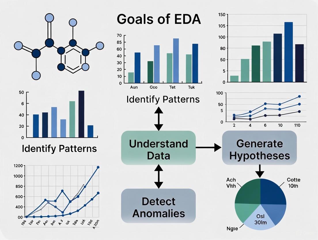
The primary goals of EDA in environmental research include: ensuring data quality before advanced analysis; understanding variable distributions and relationships; identifying spatial and temporal patterns; detecting outliers and anomalous events; informing selection of appropriate statistical techniques; and generating hypotheses for further investigation [2] [9]. By employing EDA, environmental scientists can transform raw data into actionable insights that support evidence-based decision-making for environmental management and policy development [8].
Fundamental EDA Techniques for Environmental Data
Univariate Analysis
Univariate analysis examines the distribution and properties of individual variables, forming the foundation of EDA [9]. This approach helps researchers understand data structure, identify anomalies, and determine appropriate transformations or statistical tests.
Table 1: Univariate Graphical Methods for Environmental Data
| Method | Description | Environmental Application Example | Key Information Revealed |
|---|---|---|---|
| Histograms | Graphical representation of data distribution using bins or intervals [1] | Distribution of total nitrogen concentrations in stream water [1] | Shape of distribution, central tendency, spread, gaps, skewness |
| Boxplots | Compact display of distribution based on five-number summary (min, Q1, median, Q3, max) [1] | Comparing nutrient concentrations across different watersheds | Central tendency, spread, skewness, outliers |
| Stem-and-leaf plots | Hybrid display showing both individual data points and overall distribution [2] | Preliminary analysis of small environmental datasets | Individual values, shape of distribution, gaps |
| Cumulative Distribution Functions (CDF) | Shows probability that observations are not larger than a specified value [1] | Assessing proportion of lakes exceeding water quality thresholds | Complete distribution, percentiles, exceedance probabilities |
Bivariate and Multivariate Analysis
Bivariate analysis explores relationships between two variables, while multivariate analysis examines interactions among three or more variables simultaneously [9]. These approaches are essential for understanding complex environmental systems where multiple factors interact.
Table 2: Bivariate and Multivariate Analysis Techniques
| Technique | Type | Description | Environmental Application |
|---|---|---|---|
| Scatterplots | Bivariate graphical | Plots paired observations of two variables on x-y axes [1] | Visualizing stressor-response relationships [1] |
| Scatterplot Matrix | Multivariate graphical | Multiple scatterplots displayed in matrix format [1] | Examining pairwise relationships among multiple water quality parameters |
| Correlation Analysis | Bivariate statistical | Measures strength and direction of association between variables [1] | Quantifying relationship between pollutant concentrations and biological indicators |
| Conditional Probability Analysis | Bivariate/Multivariate | Probability of an event given another event has occurred [1] | Estimating probability of biological impairment given stressor thresholds |
Advanced EDA Methodologies for Environmental Applications
Conditional Probability Analysis for Stressor Identification
Conditional Probability Analysis (CPA) provides a valuable framework for assessing relationships between environmental stressors and biological responses [1]. This technique is particularly useful when dealing with dichotomous outcomes (e.g., impaired/not impaired) and continuous stressor variables.
Methodology:
- Define Response Threshold: Establish a biologically meaningful threshold for the response variable (e.g., relative abundance of sensitive taxa < 40% indicates poor condition) [1]
- Calculate Conditional Probabilities: For each potential stressor threshold (Xc), compute P(Y|X > Xc), where Y represents the adverse biological condition
- Visualize Relationship: Plot probability of observing biological impairment against increasing stressor levels
- Interpret Pattern: Identify stressor thresholds at which probability of impairment increases substantially
Environmental Application Example: In sediment quality assessment, CPA can estimate the probability of observing benthic macroinvertebrate impairment when fine sediment percentage exceeds specific thresholds [1]. The analysis reveals how impairment probability changes with increasing stressor levels, informing management decisions about acceptable sediment thresholds.
Correlation Analysis for Multiple Stressors
Environmental systems often involve multiple, correlated stressors that jointly affect biological communities [1]. Correlation analysis helps identify these interrelationships, preventing spurious conclusions in subsequent analyses.
Protocol for Correlation Analysis:
- Select Appropriate Coefficient:
- Pearson's r: For linear relationships between normally distributed variables
- Spearman's ρ: For monotonic relationships or non-normal data
- Kendall's τ: Alternative rank-based measure with similar applications to Spearman's
- Calculate Pairwise Correlations: Compute correlations between all stressor variables
- Visualize Correlation Matrix: Create heatmap or similar visualization to identify strongly correlated stressors
- Interpret Ecological Significance: Consider whether correlations represent causal relationships or coincidental patterns
Table 3: Correlation Coefficients for Environmental Data Analysis
| Coefficient | Data Requirements | Strengths | Limitations | Interpretation |
|---|---|---|---|---|
| Pearson's r | Interval/ratio data, linear relationship, normality | Measures strength of linear relationship | Sensitive to outliers, assumes linearity | -1 to +1, with 0 indicating no linear relationship |
| Spearman's ρ | Ordinal, interval, or ratio data, monotonic relationship | Robust to outliers, no distribution assumptions | Less powerful than Pearson's for linear relationships | -1 to +1, measures monotonic relationship strength |
| Kendall's τ | Ordinal, interval, or ratio data, monotonic relationship | Handles ties better than Spearman's, more intuitive interpretation | Smaller absolute values than Spearman's for same relationship | -1 to +1, represents probability of concordance minus discordance |
Experimental Protocols for Environmental EDA
Systematic EDA Framework for Complex Environmental Datasets
Recent research demonstrates the value of systematic EDA frameworks for addressing challenges in complex environmental datasets, such as the Whole Building Life Cycle Assessment (WBLCA) dataset comprising 244 North American buildings [8]. The following protocol provides a structured approach for environmental researchers:
Phase 1: Data Characterization and Preparation
- Distinguish Attributes: Separate metadata, categorical variables, and continuous variables
- Address High Dimensionality: Identify relevant variable subsets based on research questions
- Document Data Sources: Record provenance, collection methods, and potential quality issues
Phase 2: Univariate Analysis
- Distribution Assessment: For each variable, examine distribution shape using histograms, boxplots, and Q-Q plots
- Normality Testing: Evaluate deviation from normal distribution using statistical tests and visualizations
- Summary Statistics: Calculate mean, median, standard deviation, skewness, and kurtosis
- Identify Data Issues: Flag outliers, missing values, and potential measurement errors
Phase 3: Bivariate and Multivariate Analysis
- Pairwise Relationships: Conduct correlation analysis and scatterplot examination for variable pairs
- Group Differences: Implement one-way ANOVA and post-hoc analysis for categorical groupings
- Interaction Effects: Apply two-way ANOVA to identify interacting factors
- Multivariate Visualization: Create scatterplot matrices, heatmaps, and other multivariate graphics
Phase 4: Feature Engineering and Selection
- Create Derived Variables: Develop ratios, composites, and other meaningful variable transformations
- Identify Influential Features: Use mutual information and other techniques to select important predictors
- Validate Feature Selection: Ensure selected features align with domain knowledge and research questions
Protocol for Spatial EDA of Environmental Data
Satial analysis represents a critical component of environmental EDA, enabling researchers to identify geographic patterns, hotspots, and spatial dependencies [1].
Methodology:
- Data Mapping: Create maps displaying sampling locations and variable values
- Spatial Autocorrelation: Calculate Moran's I or similar metrics to assess spatial clustering
- Variogram Analysis: For geostatistical data, examine spatial dependence structure
- Hotspot Identification: Use local indicators of spatial association (LISA) to detect significant clusters
The Environmental Scientist's EDA Toolkit
Table 4: Essential Tools for Environmental Exploratory Data Analysis
| Tool Category | Specific Tools/Software | Key Functions | Environmental Applications |
|---|---|---|---|
| Programming Languages | Python (Pandas, NumPy, Matplotlib, Seaborn) [9] | Data manipulation, statistical analysis, visualization | Water quality trend analysis, ecological indicator assessment |
| Programming Languages | R (ggplot2, dplyr, tidyr) [2] [9] | Statistical computing, advanced visualization, data tidying | Statistical analysis of monitoring data, spatial pattern detection |
| Specialized Environmental Tools | CADStat [1] | Correlation analysis, conditional probability, visualization | Stressor identification, causal analysis in biological monitoring |
| Statistical Techniques | K-means clustering [2] | Unsupervised grouping of similar observations | Classification of monitoring sites, identification of similar watersheds |
| Statistical Techniques | Principal Component Analysis (PCA) [9] | Dimension reduction for high-dimensional data | Identifying major gradients in multivariate environmental data |
| Visualization Methods | Scatterplot matrices [1] | Simultaneous display of multiple pairwise relationships | Exploring correlations among multiple water quality parameters |
| Visualization Methods | Cumulative distribution functions [1] | Display complete distribution of values | Assessing compliance with water quality standards across regions |
Data Visualization and Accessibility in Environmental EDA
Effective visualization is fundamental to EDA, enabling researchers to identify patterns, relationships, and anomalies that might be overlooked in numerical summaries [10]. For environmental data, which often involves complex spatial and multivariate relationships, accessible visual design is particularly important.
Color Contrast Guidelines for Environmental Data Visualization:
- Text Elements: Maintain contrast ratio of at least 4.5:1 for standard text against background [11] [10]
- Large Text: Use minimum contrast ratio of 4.5:1 for large-scale text (approximately 18 point or 14 point bold) [11]
- Graphical Elements: Ensure contrast ratio of at least 3:1 between adjacent data elements (e.g., bars in bar graph, pie chart segments) [10]
- Non-Color Coding: Supplement color with patterns, shapes, or direct labels to convey meaning without relying solely on color perception [10]
Accessible Visualization Practices for Environmental Data:
- Direct Labeling: Position labels adjacent to data points rather than relying on legends alone [10]
- Pattern Differentiation: Use distinct patterns (e.g., stripes, dots) in addition to color for differentiating elements
- Data Tables: Provide supplemental data tables alongside visualizations to support different learning preferences [10]
- Text Descriptions: Include alternative text for images and longer descriptions for complex visualizations [10]
Case Study: EDA of North American Building Life Cycle Assessment Data
A recent systematic EDA of Whole Building Life Cycle Assessment (WBLCA) data demonstrates the practical application of EDA principles to complex environmental datasets [8]. This study analyzed 244 real-world North American buildings using a structured EDA framework to understand embodied carbon patterns.
Key Findings and Methodological Insights:
- Weak Correlations: Embodied carbon intensity showed weak correlations with most meta-features, highlighting the complexity of environmental impact drivers [8]
- Influential Factors: Building materials and usage type emerged as the most influential factors on embodied carbon, identified through multivariate EDA techniques [8]
- Data Challenges: The EDA framework successfully addressed common environmental data challenges including high dimensionality, mixed attribute types, missing values, and outliers [8]
- Decision Support: The EDA revealed nuanced patterns that conventional simplified analyses would miss, supporting more informed decision-making for low-carbon building design [8]
This case study illustrates how systematic EDA can extract meaningful insights from complex environmental datasets, providing a foundation for advanced analysis, predictive modeling, and evidence-based environmental decision-making [8].
Exploratory Data Analysis represents an indispensable approach for identifying general patterns and unexpected features in environmental data. By employing the techniques, protocols, and tools outlined in this guide, environmental researchers can transform complex, multidimensional datasets into actionable insights that support environmental management and policy decisions. The systematic application of EDA—from basic univariate analysis to advanced multivariate techniques—ensures that subsequent statistical modeling and hypothesis testing are built upon a thorough understanding of data structure, quality, and inherent patterns. As environmental challenges grow increasingly complex, rigorous EDA will continue to play a critical role in extracting meaningful signals from noisy environmental data and informing sustainable solutions.
Detecting Outliers and Their Environmental Significance
In the realm of environmental research, Exploratory Data Analysis (EDA) serves as a critical first step for identifying general patterns, unexpected features, and outliers within datasets. [1] These outliers—observations that deviate significantly from the majority of the data—can arise from multiple sources, including sensor malfunctions, measurement inaccuracies, transmission errors, or genuine rare environmental events. [12] [13] The reliable detection of outliers is not merely a statistical exercise; it is fundamental to ensuring the integrity of subsequent analyses, from assessing model reliability to informing policy decisions for environmental conservation and public health protection. [12] This guide provides an in-depth technical framework for detecting and interpreting outliers within the broader thesis of EDA, equipping researchers with methodologies to discern erroneous measurements from critical environmental signals.
Fundamental Concepts and Importance
The Dual Nature of Outliers
In environmental datasets, outliers possess a dual nature. They can represent data quality issues that must be identified and mitigated to prevent skewed or erroneous model predictions. For instance, a malfunctioning water level sensor may report values that are physically impossible, compromising flood forecasting models. [13] Conversely, outliers can also signify critical environmental phenomena, such as a sudden spike in heavy metal concentration indicating a pollution event or an extreme rainfall measurement heralding a major storm. [12] The core challenge for researchers is to distinguish between these two types of outliers, a process that requires both robust technical methods and domain-specific knowledge.
Impact on Machine Learning Models
The presence of outliers can profoundly impact the development and performance of machine learning (ML) models designed to predict environmental conditions. Studies on predicting heavy metal (HM) contamination in soils have demonstrated that outliers can lead to inaccurate data patterns, detrimentally affecting model robustness and predictive accuracy. [12] Research shows that employing outlier detection techniques like Density-Based Spatial Clustering of Applications with Noise (DBSCAN) before model training can substantially improve the performance of ensemble algorithms such as XGBoost. For example, the R² values for predicting Chromium (Cr), Nickel (Ni), Cadmium (Cd), and Lead (Pb) were enhanced by 11.11%, 6.33%, 14.47%, and 5.68%, respectively, after outlier management. [12] This underscores the hypothesis that managing input data outliers is crucial for enhancing the precision of environmental contamination predictions.
Methodologies for Outlier Detection
A range of methodologies exists for outlier detection, from traditional statistical approaches to advanced machine learning algorithms. The choice of method depends on the data's nature, size, and distribution, as well as the availability of pre-labeled data.
Traditional Statistical and Exploratory Methods
Exploratory Data Analysis (EDA) utilizes several graphical and statistical techniques to understand variable distributions and identify potential outliers. [1]
- Boxplots: A box and whisker plot provides a compact distribution summary. The box is defined by the 25th and 75th percentiles, with a line at the median. Whiskers typically extend to a span calculated as
1.5 * (75th percentile - 25th percentile), and data points beyond this span are often identified as outliers. [1] This method is particularly useful for comparing distributions across different data subsets. - Histograms: A histogram summarizes data distribution by grouping observations into intervals (bins) and counting observations in each. Intervals with exceptionally low or high counts may indicate outliers. [1]
- Scatterplots: These graphical displays plot one variable against another, helping to visualize relationships and identify unusual observations that fall far from the general data cluster. [1]
- Q-Q Plots: Quantile-Quantile plots compare a variable's distribution to a theoretical distribution (e.g., normal distribution). Deviations from the straight line can indicate outliers, among other distributional issues. [1]
Machine Learning Approaches
Machine learning offers powerful, automated techniques for outlier detection, broadly categorized into supervised and unsupervised learning.
Unsupervised Learning: These methods are valuable when labeled data (data pre-classified as normal or outlier) are unavailable.
- Isolation Forest (IF): This algorithm is based on the principle that outliers are few and different, making them easier to isolate. It builds binary trees by randomly selecting features and split values. Samples that are isolated with fewer splits (i.e., found in shorter branch depths) are considered outliers. IF is non-parametric, has linear time complexity, and is efficient for large datasets. [13] It has been successfully applied to detect outliers in hydrological time series data from rainfall and water level stations. [13]
- DBSCAN (Density-Based Spatial Clustering of Applications with Noise): A clustering algorithm that groups together closely packed points. Points that do not belong to any cluster are labeled as noise (outliers). It is effective for identifying outliers in spatial data and has been used to improve ML model efficacy for heavy metal prediction. [12]
Supervised Learning: These methods are applicable when a labeled dataset is available for training.
- XGBoost (Extreme Gradient Boosting): An ensemble learning algorithm that can be trained on historical data containing known outlier patterns to classify new data points. In comparative studies, XGBoost demonstrated superior outlier detection performance compared to Isolation Forest when labeled data were available, yielding fewer false positives and false negatives. [13]
Table 1: Comparison of Outlier Detection Methods
| Method | Type | Key Principle | Advantages | Disadvantages |
|---|---|---|---|---|
| Boxplot | Statistical | Identifies points outside 1.5*IQR | Simple, fast, intuitive | Less effective for high-dimensional data |
| Isolation Forest | Unsupervised ML | Isolates outliers via random splits | No labels needed, efficient for large data | May struggle with high-dimensional clustered data |
| DBSCAN | Unsupervised ML | Density-based clustering | Effective for spatial data, identifies arbitrary clusters | Sensitive to hyperparameters (eps, min_samples) |
| XGBoost | Supervised ML | Ensemble tree-based classification | High accuracy with labeled data, handles complex patterns | Requires labeled training data |
Experimental Protocols and Workflows
Implementing a robust outlier detection strategy requires a structured workflow. The following protocols detail key methodologies and their application in environmental case studies.
Protocol 1: Machine Learning with Outlier Detection for Soil Heavy Metals
This protocol is adapted from studies on predicting heavy metal contamination in soils using ML and advanced outlier detection techniques. [12]
- Data Collection: Collect soil samples (e.g., 150 samples from a study region). Analyze for heavy metal concentrations (Cr, Ni, Cd, Pb) and potential influencing factors (soil characteristics, climate, geology, land use). [12]
- Data Screening: Perform initial EDA using boxplot analysis to visualize data distributions and identify obvious outliers across variables like soil pH, organic matter, and metal concentrations. [12] [1]
- Outlier Detection: Apply an outlier detection algorithm such as DBSCAN to the dataset. DBSCAN will cluster densely packed data points and mark points in low-density regions as outliers. [12]
- Model Training: Train multiple machine learning models (e.g., XGBoost, LightGBM) on the dataset both with and without the outliers identified in the previous step.
- Model Evaluation: Compare model efficacy using metrics like R² (coefficient of determination). The study demonstrated significant improvements in R² for Cr, Ni, Cd, and Pb after using DBSCAN, validating the importance of outlier management. [12]
- Feature Importance Analysis: Use the trained model (e.g., XGBoost) to determine the relative importance of different soil factors on heavy metal contents. Studies have shown soil characteristics can influence Cr (80%), Ni (72.61%), Cd (53.35%), and Pb (63.47%). [12]
- Spatial Analysis: Employ spatial analysis techniques like LISA (Local Indicators of Spatial Association) on the predicted values to identify significant contamination hotspots and understand spatial autocorrelation. [12]
Protocol 2: Quality Control of Hydrological Time Series Data
This protocol outlines a framework for quality control and outlier detection in hydrological data, such as rainfall and water levels, crucial for flood forecasting and water resource management. [13]
- Data Acquisition: Gather time series data from monitoring stations (e.g., daily rainfall and water level data from multiple stations in a river basin). [13]
- Data Preprocessing: Handle missing values by excluding intervals containing them from the model training process. [13]
- Model Selection and Application:
- If labeled data is available: Employ a supervised learning algorithm like XGBoost, trained on historical data labeled with known outlier patterns (e.g., sensor malfunctions, transmission errors). [13]
- If labeled data is unavailable: Employ an unsupervised learning algorithm like Isolation Forest (IF). IF will build multiple isolation trees to identify data points that are isolated with fewer splits as anomalies. [13]
- Validation and Implementation: Validate the model's performance by comparing its detections against known events or manual checks. Implement the chosen model within an automated quality control (AQC) system to enable real-time monitoring and outlier detection, shifting from manual processes to data-driven management. [13]
Outlier Detection and Interpretation Workflow
The Scientist's Toolkit: Essential Research Reagents and Materials
Table 2: Key Research Reagents and Computational Tools
| Item/Tool | Type | Function in Outlier Detection & Environmental Analysis |
|---|---|---|
| Soil Samples | Physical Sample | Primary matrix for laboratory analysis of heavy metal concentrations (e.g., Cr, Ni, Cd, Pb) and other soil characteristics. [12] |
| Hydrological Sensors | Field Instrument | Collects time-series data on rainfall and water levels, which are prone to outliers from malfunctions or extreme events. [13] |
| Python/R Libraries | Software | Provide implementations of statistical tests, ML algorithms (Isolation Forest, XGBoost, DBSCAN), and visualization tools (boxplots, scatterplots). [12] [13] |
| CAMS Global Reanalysis Data | Atmospheric Data | Provides coarse-resolution global data on air pollutants; used as a base for downscaling and anomaly detection projects. [14] |
| Spatial Analysis Software (e.g., GIS) | Software | Enables spatial EDA and the application of techniques like LISA and Moran's I to identify contamination hotspots and spatial outliers. [12] |
Visualization of Method Selection and Relationships
Choosing the correct outlier detection method is a critical decision point in the analytical workflow. The following diagram outlines the logical decision process based on data characteristics and research goals.
Method Selection for Outlier Detection
Within the framework of Exploratory Data Analysis, the detection and correct interpretation of outliers are foundational to robust environmental research. Whether through traditional statistical graphics or advanced machine learning techniques like Isolation Forest and XGBoost, managing outliers directly enhances the accuracy of predictive models for soil contamination, hydrological forecasting, and air quality assessment. [12] [13] The experimental protocols and workflows detailed in this guide provide a roadmap for researchers to systematically improve data integrity. By effectively identifying and reconciling these anomalous data points, scientists can ensure their analyses yield reliable, actionable insights, ultimately supporting informed decisions for environmental conservation and public health protection.
Examining Variable Distributions Through Histograms, Boxplots, and Q-Q Plots
Exploratory Data Analysis (EDA) is an essential first step in any data analysis, aimed at identifying general patterns, unexpected features, and outliers within datasets [1]. In the context of environmental research, where data is often complex and influenced by multiple natural and anthropogenic factors, understanding the distribution of variables is not merely preliminary work but a foundational component of a scientifically defensible analysis [15]. This initial exploration helps researchers understand the underlying structure of their data, check the assumptions required for more sophisticated statistical techniques, and design analyses that yield meaningful, reliable results about environmental conditions [1] [2].
The process of establishing soil background values, for instance, relies heavily on understanding data distributions, as many statistical tests have underlying assumptions about how the data is distributed [15]. Applying a statistical test to a dataset that does not meet its distributional assumptions can produce erroneous and misleading conclusions, potentially compromising environmental decision-making [15]. This guide will detail the methodologies for using three pivotal graphical tools—histograms, boxplots, and Q-Q plots—to examine variable distributions effectively.
Key Graphical Methods for Distribution Analysis
Histograms
A histogram is a graphical representation that summarizes the distribution of a continuous variable by grouping observations into intervals (also called classes or bins) and counting the number of observations in each interval [1]. It provides a visual impression of the shape, spread, and central tendency of the data, making it easy to identify patterns such as skewness, modality, and the presence of gaps.
Detailed Methodology
The construction of a histogram involves the following steps:
- Data Preparation: Begin with a single continuous variable. The EPA's analysis of log-transformed total nitrogen from the EMAP-West Streams Survey is a prime environmental example [1].
- Interval (Bin) Selection: Choose the number and width of the intervals. The appearance and interpretability of a histogram can depend significantly on this choice. While there is no single fixed rule, common strategies include:
- Using a rule of thumb like Sturges' formula or the Square-root choice for the number of bins.
- Experimenting with different bin widths in software to see which best reveals the underlying structure of the data without being too smooth or too rough.
- Axis Labeling:
- The x-axis represents the range of the data, divided into the chosen intervals.
- The y-axis can represent the frequency (count of observations), the percent or fraction of the total, or the density (where the area of the bar represents the relative frequency) [1].
- Plotting: Draw a bar for each interval, with the height corresponding to the count (or proportion) of observations within that interval. The bars are typically drawn adjacent to each other to emphasize the continuous nature of the data.
Table 1: Key Characteristics and Interpretation of Histograms
| Characteristic | Description | Interpretation in Environmental Context |
|---|---|---|
| Symmetry | Whether the distribution is mirror-imaged around a central point. | Asymmetrical, skewed distributions are common for natural soil concentrations (often positively skewed) [15]. |
| Modality | The number of prominent peaks (modes). | A single peak (unimodal) may suggest one population; multiple peaks (bimodal/multimodal) can suggest multiple populations or mixtures of materials, which should be investigated [15]. |
| Skewness | The tendency of the distribution to tail off to one side. | Positive skew (tail to the right) indicates many low values and a few very high values, common for pollutant concentrations. |
| Gaps | Intervals with no observations. | May indicate data quality issues or the presence of different geological strata or source populations. |
Boxplots (Box-and-Whisker Plots)
A boxplot (or box-and-whisker plot) provides a compact, standardized visual summary of a distribution based on a five-number summary: minimum, first quartile (Q1), median, third quartile (Q3), and maximum [1] [2]. Its primary strength lies in its ability to highlight the central value, spread, and potential outliers in the data, making it particularly useful for comparing distributions across different subsets (e.g., soil samples from different depths or regions) [1].
Detailed Methodology
The construction of a standard boxplot follows this protocol [1]:
- Calculate the Five-Number Summary:
- Minimum: The smallest data point, excluding outliers.
- First Quartile (Q1): The 25th percentile; 25% of the data fall below this value.
- Median (Q2): The 50th percentile; the middle value of the dataset.
- Third Quartile (Q3): The 75th percentile; 75% of the data fall below this value.
- Maximum: The largest data point, excluding outliers.
- Draw the Box:
- A box is drawn from Q1 to Q3. The length of this box is the Interquartile Range (IQR), which contains the middle 50% of the data.
- A line is drawn inside the box at the median.
- Draw the Whiskers:
- The upper whisker extends from Q3 to the largest data point that is less than or equal to
Q3 + 1.5 * IQR. - The lower whisker extends from Q1 to the smallest data point that is greater than or equal to
Q1 - 1.5 * IQR.
- The upper whisker extends from Q3 to the largest data point that is less than or equal to
- Plot Outliers:
- Any data points that fall outside the whisker span (i.e., greater than
Q3 + 1.5 * IQRor less thanQ1 - 1.5 * IQR) are plotted as individual points or dots. These are considered potential outliers and warrant further investigation in an environmental context [1].
- Any data points that fall outside the whisker span (i.e., greater than
Table 2: Components of a Boxplot and Their Scientific Meaning
| Component | Statistical Value | Interpretation |
|---|---|---|
| Box | Spans the Interquartile Range (IQR) from Q1 to Q3. | Represents the middle 50% of the data, showing the core spread of the distribution. |
| Median Line | The middle value of the dataset (50th percentile). | Indicates the central tendency of the data. A median not in the center of the box suggests skewness. |
| Whiskers | Extend to the minimum and maximum values within 1.5 IQR from the quartiles. | Show the range of typical data values. The length of the whiskers indicates the variability of the lower and upper quarters of the data. |
| Outliers | Data points beyond the whiskers. | Potential anomalies that may be due to measurement error, contamination, or rare natural events. Must be investigated, not automatically removed. |
Quantile-Quantile (Q-Q) Plots
A Q-Q plot (or probability plot) is a graphical technique used to compare a sample dataset to a theoretical distribution (e.g., the normal distribution) or to compare two sample datasets [1] [15]. It is one of the most powerful tools for assessing whether a dataset follows a particular distribution, which is a critical assumption for many parametric statistical tests used in environmental modeling [15].
Detailed Methodology
The protocol for creating a Q-Q plot against a theoretical normal distribution is as follows:
- Data Preparation and Sorting: Take the variable of interest and sort the data points in ascending order.
- Theoretical Quantile Calculation: For each ordered data point, calculate its corresponding theoretical quantile (z-score) from a standard normal distribution. This is often done using a plotting position formula like
(i - 0.5) / n, whereiis the rank of the observation andnis the sample size. - Plotting: Plot the points on a scatterplot where:
- The x-axis represents the theoretical quantiles (from the normal distribution).
- The y-axis represents the actual observed quantiles (the sorted data values).
- Reference Line: A reference line (often a 45-degree line) is added to the plot, representing where the points would lie if the data perfectly followed the theoretical distribution.
Interpretation
- Data Points Follow the Line: If the plotted points fall approximately along the straight reference line, it suggests the data are consistent with the theoretical distribution (e.g., normal) [1].
- Systematic Deviations from the Line: Curvature at the ends of the Q-Q plot indicates skewness. S-shaped curves indicate heavier or lighter tails than the theoretical distribution. The EPA highlights the utility of Q-Q plots in demonstrating how a log-transform can make total nitrogen data better approximate a normal distribution [1].
- Identification of Multiple Populations: The presence of distinct breaks or curves in the Q-Q plot can suggest that the data come from more than one underlying population, a key consideration when defining a target population for background soil studies [15].
Practical Workflow and Implementation
The following diagram illustrates a logical workflow for employing these three graphical methods in sequence to thoroughly examine a variable's distribution.
Graphical Workflow for Distribution Analysis
The Scientist's Toolkit: Essential Reagents and Materials
Table 3: Key Research Reagent Solutions for Distributional Analysis
| Tool / Reagent | Function / Purpose | Example in Environmental Research |
|---|---|---|
| Statistical Software (R/Python) | Provides the computational environment to generate visualizations and calculate summary statistics. | R with ggplot2 for creating publication-quality histograms and boxplots. Python with SciPy and matplotlib for generating Q-Q plots and assessing normality [2]. |
| Probability Distribution Tables/Functions | Serves as the theoretical benchmark against which empirical data is compared. | The normal distribution is a common benchmark, but lognormal or gamma distributions may be more appropriate for skewed environmental data like soil contaminant concentrations [15]. |
| Data Visualization Guidelines | A set of principles to ensure graphs are accurate, clear, and accessible. | Using sufficient color contrast (≥ 4.5:1 for text) for readability [16], employing intuitive colors (e.g., green for vegetation indices), and using grey for less important context elements [17]. |
| ProUCL Software (USEPA) | A specialized statistical software package for environmental applications. | Used for calculating background threshold values, especially with datasets that are skewed and not normally distributed [15]. |
Critical Data Considerations for Environmental Research
Before applying any graphical or statistical method, data must meet certain quality and characteristic standards to ensure defensible results [15].
- Minimum Sample Size: A sufficient sample size is critical. While some guidance suggests a minimum of 8–10 samples to calculate statistical parameters, the typical heterogeneity of soils leads many agencies to recommend at least 20 samples for a robust analysis [15].
- Data Representativeness: The dataset must be a random, unbiased sample of the target population (e.g., arsenic in a specific soil type). Combining data from different populations (e.g., shallow and deep soils) without justification can lead to erroneous background values [15]. Graphical displays like Q-Q plots and histograms are key tools for identifying the presence of multiple populations [15].
- Data Independence: A core assumption for most statistical tests is that each sample is independent and not influenced by other measurements [15]. Sampling design must account for this.
Histograms, boxplots, and Q-Q plots are not merely isolated graphics but are interconnected tools that, when used in concert, provide a comprehensive picture of a variable's distribution. For environmental researchers and scientists, this rigorous exploratory process is indispensable. It confirms that subsequent, more complex statistical analyses and models—which often form the basis for risk assessments and regulatory decisions—are built upon a sound and well-understood data foundation. By following the detailed methodologies and workflows outlined in this guide, professionals can ensure their findings are both statistically valid and scientifically defensible.
Generating Hypotheses About Stressor-Response Relationships in Environmental Systems
In environmental research, stressor-response relationships describe how biological systems change in response to varying levels of environmental stressors. As defined by the U.S. Environmental Protection Agency (EPA), this relationship follows the fundamental principle that as exposure to a stressor increases, the intensity or frequency of a biological effect increases correspondingly [18]. Understanding these relationships is a core component of causal assessment in environmental systems, enabling researchers to identify anthropogenic impacts and guide restoration efforts.
This process is intrinsically linked to Exploratory Data Analysis (EDA). EDA serves as the critical first step in identifying general patterns, outliers, and unexpected features within environmental datasets [1]. In biological monitoring, where sites are often affected by multiple, co-occurring stressors, initial explorations of stressor correlations are essential before attempting to relate stressor variables to biological responses. EDA provides the foundational insights that inform the development of robust, testable causal hypotheses about the mechanisms affecting ecological communities.
Foundational Concepts and Evidence Integration
The evaluation of stressor-response hypotheses typically relies on multiple lines of evidence, which can be categorized based on the source and nature of the data. Two primary types of evidence used in frameworks like the EPA's CADDIS are detailed below.
Table 1: Types of Stressor-Response Evidence from Field Studies
| Evidence Type | Definition | Supporting Evidence Example | Weakening Evidence Example |
|---|---|---|---|
| Stressor-Response from the Field [18] | Relationships derived from data collected at the impaired site or from a set of spatially contiguous sites. | Mayfly taxonomic richness correlates inversely with % embeddedness; high embeddedness sites have low taxa counts. | No clear pattern exists between % embeddedness and mayfly richness; sites with high and low embeddedness have similar taxa counts. |
| Stressor-Response from Other Field Studies [19] | Relationships derived from other, similar field studies, used to assess if the stressor at the impaired site is at levels sufficient to cause the observed effect. | State monitoring data shows mayfly richness declines once fine silt coverage exceeds 10%; at the case site, coverage is 15%. | State monitoring data shows mayfly richness declines once fine silt coverage exceeds 10%; at the case site, coverage is only 5%. |
Hypotheses are evaluated by scoring the strength and consistency of the evidence. The following table provides a generalized scoring framework for stressor-response relationships from field data.
Table 2: Scoring Evidence for Stressor-Response Relationships from Field Data [18]
| Finding | Interpretation | Score |
|---|---|---|
| A strong effect gradient is observed relative to exposure to the candidate cause at spatially linked sites, and the gradient is in the expected direction. | Strongly supports the case, but is not convincing due to potential confounding. | ++ |
| A weak effect gradient is observed at spatially linked sites, OR a strong gradient is observed at non-linked sites in the expected direction. | Somewhat supports the case, but not strongly supportive due to potential confounding or random error. | + |
| An uncertain effect gradient is observed. | Neither supports nor weakens the case, as the evidence is ambiguous. | 0 |
| An inconsistent effect gradient is observed at spatially linked sites, OR a strong gradient is observed at non-linked sites in an unexpected direction. | Somewhat weakens the case, but not strongly weakening due to potential confounding or error. | - |
| A strong effect gradient is observed at spatially linked sites, but the relationship is not in the expected direction. | Strongly weakens the case, but is not convincing due to potential confounding. | -- |
Methodological Workflow for Hypothesis Generation
The process of generating and evaluating stressor-response hypotheses involves a sequence of steps from initial data exploration to causal assessment. The following diagram visualizes this core analytical workflow.
Exploratory Data Analysis (EDA) Techniques
EDA is the essential first step for generating initial hypotheses about potential stressors. Key graphical methods include [1]:
- Histograms and Boxplots: Used to examine the distribution of individual stressor and response variables. Boxplots are particularly useful for comparing distributions across different site categories (e.g., reference vs. impaired).
- Scatterplots: Fundamental for visualizing the relationship between pairs of variables (e.g., a stressor on the x-axis and a biological response on the y-axis). Scatterplots can reveal nonlinear relationships, non-constant variance, and outliers that may influence subsequent statistical analyses.
- Scatterplot Matrices: A convenient way to display pairwise relationships between several variables simultaneously, providing a broad overview of potential interactions in the dataset.
- Quantile-Quantile (Q-Q) Plots: Used to check whether a variable follows a particular theoretical distribution (e.g., normality), which can inform the selection of appropriate statistical tests.
Statistical Analysis of Relationships
Once potential relationships are identified visually, statistical methods are employed to quantify them.
- Correlation Analysis: Measures the covariance of two random variables. Pearson's product-moment correlation coefficient (r) measures linear association, while Spearman's rank-order coefficient (ρ) and Kendall's tau (τ) are more robust to outliers and non-linear, monotonic relationships [1].
- Conditional Probability Analysis (CPA): Used to estimate the probability of observing a biological effect (Y) given that a particular stressor condition (X) is present or exceeds a threshold [1]. This requires dichotomizing the biological response variable (e.g., defining "poor" vs. "good" condition). The probability is calculated as P(Y|X) = P(X and Y) / P(X).
- Regression Techniques: Field stressor-response relationships are commonly analyzed with regression. Quantile regression may be particularly useful for identifying upper or lower limits of a biological response across a gradient of stressor intensity [19].
Successfully navigating a stressor-response analysis requires a suite of conceptual and statistical tools. The following table outlines essential resources for environmental researchers.
Table 3: Research Reagent Solutions for Stressor-Response Analysis
| Tool or Technique | Primary Function | Application Context |
|---|---|---|
| Scatterplots & Correlation Coefficients [1] | Visually and statistically assess the relationship between two continuous variables. | Initial exploration of data to identify potential causal links and data issues (e.g., outliers, non-linearity). |
| Conditional Probability Analysis (CPA) [1] | Estimate the probability of a biological effect given the presence or level of a stressor. | Useful when the response variable can be meaningfully dichotomized (e.g., impaired/not impaired). |
| Boxplots (Box and Whisker Plots) [1] | Compact visual summary of a variable's distribution, including median, quartiles, and outliers. | Comparing the distribution of a stressor or response metric across different site groups or conditions. |
| Multivariate Visualization (e.g., PCA) [18] [19] | Reduce dimensionality and group highly correlated stressors to understand co-occurrence patterns. | Addressing confounding when multiple stressors co-vary, helping to identify groups of stressors that increase/decrease together. |
| CADStat [1] | A menu-driven software package that provides tools for calculating correlations, conditional probabilities, and other statistical measures relevant to causal analysis. | Applying standardized analytical methods within the EPA CADDIS causal assessment framework. |
Visualization and Accessibility in Scientific Communication
Effective communication of stressor-response findings is critical. Adhering to principles of accessible data visualization ensures that charts and diagrams are understandable by the broadest possible audience [10].
- Color and Contrast: Use colors with a high contrast ratio (at least 4.5:1 for text and 3:1 for graphical elements) [10]. Never use color as the sole means of conveying information; supplement with patterns, shapes, or direct labels [10].
- Clarity and Annotation: Eliminate visual clutter and use descriptive titles, subtitles, and annotations. Annotations should explain not only "what" is being measured but "why" it matters and "how" to read the chart, using plain language and avoiding acronyms [20].
- Accessible Flowcharts: For complex diagrams, provide a text-based alternative. This can be an ordered list with "If X, then go to Y" language or a structured heading hierarchy that conveys the same logical flow [21]. The alt text for a flowchart image should summarize the overall relationship as you would describe it over the phone [21].
The rigorous generation and testing of hypotheses about stressor-response relationships form the bedrock of scientific causal assessment in environmental systems. This process is inherently iterative, grounded in thorough exploratory data analysis, and reliant on the integration of multiple lines of evidence. By applying a structured workflow—from initial data exploration using EDA techniques, through quantitative analysis with correlation and regression, to critical evaluation against evidence from other studies—researchers can move from observational patterns to defensible causal inferences. Adhering to best practices in data visualization and accessibility ensures that these complex relationships are communicated effectively, fostering robust scientific discourse and informing sound environmental decision-making.
Assessing Data Quality and Recognizing Measurement Limitations
Exploratory Data Analysis (EDA) serves as a critical first step in environmental research, establishing a foundation for robust scientific conclusions. This approach identifies general patterns, outliers, and unexpected features within datasets before formal statistical modeling is conducted [1]. In the context of environmental monitoring, where sites are often affected by multiple interacting stressors, initial explorations of data quality and variable relationships are paramount. Understanding measurement limitations at this early stage guides the selection of appropriate analytical techniques and ensures that subsequent analyses yield meaningful, reliable results that accurately represent complex environmental systems [1].
The growing integration of big data analytics into environmental quality monitoring further amplifies the importance of rigorous data assessment [22]. As researchers increasingly employ advanced data science techniques and machine learning algorithms to analyze vast environmental datasets, establishing robust protocols for evaluating data quality becomes essential for effective evidence-based policymaking [22]. This technical guide provides environmental researchers with comprehensive methodologies for assessing data quality and recognizing measurement limitations within the EDA framework, enabling more transparent and reproducible environmental science.
Foundational Concepts in Data Quality Assessment
Data Quality Dimensions in Environmental Context
Data quality in environmental research encompasses multiple dimensions that collectively determine the fitness-for-use of datasets for specific analytical purposes. Key dimensions include:
- Completeness: The degree to which expected data values are present without gaps or missing observations, critical for time-series analysis of environmental parameters.
- Accuracy: The closeness of measured values to true values or accepted reference standards, particularly important for chemical concentration measurements and sensor data.
- Precision: The repeatability of measurements under unchanged conditions, relevant for laboratory analyses and field instrument calibration.
- Consistency: The absence of contradictions in datasets across time and space, essential for long-term environmental monitoring studies.
- Representativeness: The extent to which data accurately reflects the environmental population or phenomenon being studied, crucial for spatial analyses and ecological surveys.
FAIR Principles for Environmental Data
Adhering to Findable, Accessible, Interoperable, and Reusable (FAIR) principles significantly enhances data quality in environmental research [23]. Implementing community-centric metadata reporting formats makes Earth and environmental science data more transparent and reusable, addressing critical interoperability challenges that often hinder data integration across disciplines [23]. These standardized formats provide guidelines for consistently formatting data within specific environmental science domains, facilitating both human understanding and machine-actionability of complex environmental datasets.
Table 1: FAIR Principles Implementation for Environmental Data Quality
| Principle | Quality Dimension Addressed | Implementation in Environmental Research |
|---|---|---|
| Findable | Completeness | Persistent identifiers (DOIs), Rich metadata, Indexed in searchable repositories |
| Accessible | Representativeness | Standardized retrieval protocols, Authentication and authorization where appropriate, Long-term preservation |
| Interoperable | Consistency | Use of controlled vocabularies, Standard data formats, Qualified references to other metadata |
| Reusable | Accuracy | Multiple attributes of provenance, Detailed usage licenses, Community reporting formats |
Methodologies for Assessing Data Quality
Distribution Analysis Techniques
Examining how values of different variables are distributed represents an essential initial step in EDA for assessing data quality [1]. Multiple graphical approaches reveal distribution characteristics that inform both quality assessment and subsequent analytical choices:
Histograms summarize data distribution by placing observations into intervals and counting observations in each interval [1]. The y-axis can represent number of observations, percent of total, fraction of total, or density. In environmental applications, histograms can reveal measurement limitations such as detection limit effects, where values cluster at instrument detection thresholds.
Boxplots provide compact distribution summaries through five-number summaries (minimum, first quartile, median, third quartile, maximum) [1]. These visualizations are particularly valuable for comparing distributions across different environmental subsets (e.g., sampling sites, time periods) and identifying potential measurement errors appearing as extreme outliers.
Quantile-Quantile (Q-Q) Plots graphically compare variable distributions to theoretical distributions or to other variables [1]. A common application checks normality assumptions, with deviations from linearity indicating distributional issues that may suggest measurement limitations or need for data transformation before analysis.
Cumulative Distribution Functions (CDF) display the probability that observations of a variable are not larger than a specified value [1]. In environmental monitoring with probability sampling designs, weighted CDFs (using inclusion probabilities as weights) provide population-level estimates that account for sampling design, addressing representativeness limitations.
Relationship Analysis Methods
Scatterplots graphically display matched data with one variable on each axis, visualizing relationships and identifying potential data quality issues [1]. These plots reveal characteristics such as nonlinear relationships or non-constant variance that influence analytical choices and may indicate measurement limitations in environmental datasets.
Correlation Analysis measures covariance between two random variables in matched data [1]. Different correlation coefficients serve complementary roles in data quality assessment:
- Pearson's product-moment correlation coefficient (r): Measures degree of linear association
- Spearman's rank-order correlation coefficient (ρ): Uses data ranks, more robust to outliers
- Kendall's tau (τ): Represents probability that two variables are ordered nonrandomly
Different correlation coefficients may provide divergent estimates depending on data distribution, offering insights into potential measurement limitations and data quality issues [1].
Conditional Probability Analysis (CPA) applies conditional probability concepts to dichotomized environmental response variables [1]. This technique requires defining thresholds that categorize samples into two classes (e.g., impaired/unimpaired), then estimating the probability of observing environmental impairment given particular stressor conditions. CPA is most meaningful when applied to field data collected using randomized, probabilistic sampling designs [1].
Table 2: Statistical Measures for Data Quality Assessment in Environmental Research
| Method | Primary Quality Dimension | Calculation | Application Context |
|---|---|---|---|
| Pearson's r | Consistency | r = Σ[(xi - x̄)(yi - ȳ)] / [√Σ(xi - x̄)² √Σ(yi - ȳ)²] | Linear relationships between normally distributed variables |
| Spearman's ρ | Consistency | ρ = 1 - [6Σd_i² / (n(n² - 1))] where d = rank difference | Monotonic relationships, non-normal data, ordinal measurements |
| Kendall's τ | Consistency | τ = (C - D) / √[(C + D + Tx)(C + D + Ty)] where C=concordant pairs, D=discordant pairs | Small sample sizes, many tied ranks |
| Conditional Probability | Accuracy | P(Y|X) = P(Y∩X) / P(X) where Y=response, X=stressor | Stressor identification in causal analysis with dichotomous response |
Experimental Protocols for Data Quality Assessment
Protocol for Distribution-Based Quality Assessment
Purpose: Systematically evaluate data quality through distribution analysis to identify measurement limitations and inform analytical approaches.
Materials Required:
- Environmental dataset with relevant variables
- Statistical software (R, Python, or specialized tools like CADStat [1])
- Visualization capabilities
Procedure:
- Generate distribution visualizations: Create histograms, boxplots, and Q-Q plots for all key variables [1].
- Assess normality: Examine Q-Q plots for deviations from linearity indicating non-normality.
- Identify outliers: Use boxplots to detect extreme values requiring verification.
- Compare subsets: Generate separate boxplots for different sampling locations, time periods, or experimental conditions.
- Evaluate transformations: Apply appropriate transformations (e.g., log transformation for environmental concentration data) and reassess distributions.
- Document findings: Record distribution characteristics, identified outliers, and transformation decisions.
Protocol for Relationship-Based Quality Assessment
Purpose: Identify relationships between variables and detect potential data quality issues through correlation and conditional probability analysis.
Materials Required:
- Matched environmental dataset with stressor and response variables
- Statistical software with correlation and probability calculation capabilities
- Threshold values for dichotomizing response variables (for CPA)
Procedure:
- Create scatterplot matrices: Generate pairwise scatterplots for multiple variables to visualize relationships [1].
- Calculate correlation coefficients: Compute Pearson's, Spearman's, and Kendall's coefficients for variable pairs.
- Compare coefficient patterns: Identify discrepancies between coefficients that may indicate nonlinear relationships or outliers.
- Dichotomize response variables: Apply scientifically-defensible thresholds to categorize response variables (e.g., biologically impaired/unimpaired) [1].
- Compute conditional probabilities: Calculate probabilities of observing response categories given stressor conditions.
- Visualize CPA results: Plot conditional probabilities against stressor gradients to identify potential thresholds.
Visualization of Data Quality Assessment Workflows
Figure 1: Comprehensive workflow for assessing data quality and recognizing measurement limitations in environmental research, integrating distribution analysis and relationship assessment methodologies.
Table 3: Research Reagent Solutions for Environmental Data Quality Assessment
| Tool/Resource | Function | Application Context |
|---|---|---|
| CADStat [1] | Menu-driven package for data visualization and statistical methods | Calculating correlations, conditional probabilities; EDA for environmental data |
| ESS-DIVE Reporting Formats [23] | Community-centric (meta)data reporting formats | Standardizing data structure and metadata for FAIR environmental data |
| Scatterplot Matrices [1] | Multiple scatterplots displayed in matrix format | Visualizing pairwise relationships between multiple variables simultaneously |
| Probability Sampling Designs [1] | Statistical sampling approaches with known inclusion probabilities | Ensuring data representativeness for population-level inference |
| FAIR Data Principles [23] | Guidelines for Findable, Accessible, Interoperable, Reusable data | Enhancing data transparency, reproducibility, and reuse potential |
| Community Crosswalks [23] | Tabular maps of existing data standards and resources | Identifying gaps in standards and harmonizing variables across datasets |
Implementing systematic approaches to assess data quality and recognize measurement limitations represents a fundamental component of exploratory data analysis in environmental research. Through distribution analysis, relationship assessment, and adherence to FAIR data principles, researchers can ensure their datasets support robust scientific conclusions and evidence-based environmental policymaking. The integration of big data analytics into environmental quality monitoring [22] makes these rigorous assessment protocols increasingly vital for deriving meaningful insights from complex environmental datasets. As environmental challenges grow more complex, systematic data quality assessment enables researchers to accurately characterize environmental systems, identify emerging threats, and develop effective management strategies supported by high-quality, trustworthy data.
From Theory to Practice: Essential EDA Methods for Environmental Applications
Exploratory Data Analysis (EDA) is an essential first step in any data-driven environmental research project. It involves investigating data sets to summarize their main characteristics, often using visual methods to discover patterns, spot anomalies, test hypotheses, and check assumptions before formal modeling [2]. Within the environmental sciences, EDA is particularly crucial due to the complexity, volume, and inherent spatiotemporal variability of ecological and climatic data [24] [1]. This technical guide details the application of three foundational EDA visualization techniques—scatterplots, histograms, and boxplots—within the context of environmental research, providing researchers with detailed methodologies and practical frameworks for their implementation.
Core Visualization Techniques for Environmental Data
The following table summarizes the primary functions and environmental data applications of the three core visualization techniques.
Table 1: Core Visualization Techniques for Environmental Data Analysis
| Visualization Type | Primary Function in EDA | Common Environmental Data Applications | Key Insights Revealed |
|---|---|---|---|
| Scatterplot [25] [1] | Display relationships or correlations between two continuous variables. | Marketing spend vs. sales; Customer acquisition cost (CAC) vs. lifetime value (LTV) [25]. | Trends, outliers, clusters, and the strength/direction of correlations between variables. |
| Histogram [25] [1] | Show how values are distributed across ranges or bins. | Age demographics; Emergency department wait times; Pollution level distributions; Rainfall patterns [25] [26]. | Whether data is normally distributed, skewed, or multi-modal (having multiple peaks). |
| Boxplot (Box & Whisker) [1] [27] | Provide a compact summary of a variable's distribution. | Comparing distributions across different groups; Summarizing massive datasets like historical temperature records [27]. | Central tendency, spread, skewness, and identification of outliers across groups or over time. |
Technical Protocols and Application in Environmental Research
Scatterplots
3.1.1 Protocol for Creation and Analysis To create a scatterplot, matched data pairs are plotted with the independent variable on the horizontal (X) axis and the dependent variable on the vertical (Y) axis [1]. The resulting cloud of points is then analyzed for its overall pattern. The Pearson (r), Spearman (ρ), or Kendall (τ) correlation coefficients can be calculated to measure the degree of association, where a value of 0 indicates no linear relationship, a positive coefficient indicates a positive relationship, and a negative coefficient indicates a negative relationship [1]. The magnitude of the coefficient indicates the strength of the association. Scatterplots are highly effective for identifying potential issues in the data, such as outliers that can influence subsequent statistical analyses [1].
3.1.2 Application to Environmental Data In environmental science, scatterplots are indispensable for revealing functional relationships between variables. For example, a scatterplot can be used to examine the correlation between marketing spend and sales, or to plot customer acquisition cost (CAC) against lifetime value (LTV) to identify distinct customer clusters [25]. They help in understanding stressor-response relationships in causal analysis, such as investigating how a biological response metric changes with increasing levels of a chemical stressor [1]. When analyzing air quality, scatterplots can help find relationships between different pollutants or between urbanization levels and air quality indices [24] [26].
Histograms
3.2.1 Protocol for Creation and Analysis A histogram is constructed by dividing the range of a continuous variable into a series of consecutive, non-overlapping intervals (bins or classes) and counting the number of observations that fall into each interval [1]. The y-axis can represent the count (frequency), percent, fraction, or density of observations in each bin. The choice of bin number and width can significantly impact the histogram's appearance and interpretation. A histogram allows for a quick assessment of the underlying distribution of the data (e.g., normal, skewed), its modality (e.g., unimodal, bimodal), and the presence of gaps or unusual values [1].
3.2.2 Application to Environmental Data Histograms are used to understand the distribution of environmental parameters. A classic application is analyzing the distribution of pollution levels, such as PM2.5 concentrations, across a set of monitoring sites to see if most areas are exposed to moderate levels or if there is a wide spread [26]. They can also be used to analyze rainfall patterns to understand the frequency of different precipitation amounts [26]. Furthermore, as demonstrated in a hospital analysis, a histogram of emergency department wait times might reveal a bimodal distribution, indicating two distinct patient case types that require different staffing models [25]. This principle can be applied to environmental data, such as analyzing the distribution of a specific pollutant to identify multiple source types.
Boxplots
3.3.1 Protocol for Creation and Analysis A boxplot, or box-and-whisker plot, visually represents the five-number summary of a dataset: the minimum, first quartile (25th percentile), median (50th percentile), third quartile (75th percentile), and maximum [1] [27]. The box itself spans the interquartile range (IQR) between Q1 and Q3, with a line marking the median. The "whiskers" typically extend from the box to the smallest and largest values within 1.5 * IQR from the lower and upper quartiles, respectively. Data points beyond the whiskers are often plotted as individual points and considered potential outliers [1]. Boxplots are particularly powerful for comparing the distributions of a variable across different categories or groups side-by-side [1].
3.3.2 Application to Environmental Data Boxplots are invaluable in climatology for summarizing large datasets. For instance, hourly or daily temperature records can be aggregated into monthly or annual boxplots, making long-term trends in central tendency and variability manageable and interpretable [27]. They help researchers analyze summer average temperatures across various European countries, showing not just the average but also the variability and extremes for each region [27]. In broader environmental contexts, boxplots are ideal for comparing measures like nutrient concentrations across different watersheds or species richness across different habitat types, instantly revealing differences in median, spread, and skewness.
Table 2: Essential Tools and Reagents for Environmental Data Analysis
| Tool/Reagent | Category | Primary Function in Analysis |
|---|---|---|
| R & Python [24] [2] | Programming Language | Provide flexible environments for statistical computing, graphics, and data manipulation (e.g., using lubridate in R for date-time formatting) [24]. |
| IBM watsonx.data [2] | Data Lakehouse | A hybrid data store to unify and scale analytics and AI across all enterprise data. |
| Spreadsheets (Excel/Google Sheets) [24] | Data Management & Simple Analysis | Serve as a basic data management system (DMS) for ingesting, processing, and performing simple visualizations on smaller datasets [24]. |
| Power BI [25] [28] | Business Intelligence | A robust visualization engine for building interactive dashboards and reports, enabling rapid development of complex charts. |
| Tableau [25] [28] | Business Intelligence | Known for high visual quality, it is used for creating shareable, interactive visualizations from large datasets. |
| CADStat [1] | Statistical Software | A menu-driven package offering specific data visualization and statistical methods, including tools for calculating correlations and conditional probabilities. |
| ColorBrewer & cividis | Color Palette | Provides colorblind-friendly palettes and sequential/diverging color schemes critical for accurate and accessible data representation [24]. |
| Berkeley Earth Surface Temperature [27] | Data Source | Provides access to large, aggregated climate datasets (e.g., 1.6 billion temperature reports) for analysis. |
Scatterplots, histograms, and boxplots are foundational tools in the environmental scientist's EDA toolkit. Their disciplined application, following the outlined protocols, allows researchers to move beyond raw data to actionable understanding. By effectively revealing distributions, correlations, and comparisons, these visualizations form the critical first step in generating robust, data-driven insights into complex environmental systems, from air quality and climate change to ecosystem health. The iterative process of exploration and visualization is not merely a preliminary step but a core scientific activity that ensures subsequent analytical models and conclusions are built upon a firm and insightful understanding of the data.
Exploratory Data Analysis (EDA) is an essential first step in any environmental data analysis, aimed at identifying general patterns, detecting outliers, and understanding underlying data structures before formal hypothesis testing [1]. Within this framework, correlation analysis serves as a fundamental methodological approach for quantifying the strength and direction of associations between environmental variables. Understanding these relationships is crucial when investigating complex environmental systems where multiple stressors interact, as sites are likely to be affected by multiple, often correlated, influencing factors [1] [5].
The formation of spatiotemporal patterns in environmental quality often results from long-term interactions between natural factors and human activities [29]. For example, in assessing ecological environmental quality (EEQ) in Myanmar, researchers found significant interactions between factors such as elevation, slope, net primary productivity, and human footprint [29]. Similarly, studies in the Liaohe River Basin have demonstrated complex interactions among ecosystem services like carbon storage, food production, habitat quality, soil retention, and water yield [30]. Correlation analysis provides researchers with the statistical tools to detect, measure, and initially characterize these complex relationships, forming the foundation for more sophisticated causal analyses and mechanistic models.
Foundations of Correlation Analysis
Core Concepts and Mathematical Basis
Correlation analysis is a method for measuring the covariance of two random variables in a matched data set [1]. This covariance is typically expressed as a correlation coefficient—a unitless number ranging from -1 to +1 that quantifies the degree of association between variables X and Y. The magnitude of the coefficient indicates the strength of the association, while the sign indicates the direction of the relationship [1].
The mathematical foundation of correlation analysis centers on several key coefficients:
- Pearson's product-moment correlation coefficient (r): Measures the degree of linear association between two continuous variables with approximately normal distributions.
- Spearman's rank-order correlation coefficient (ρ): A non-parametric measure that uses the ranks of the data, making it more robust to outliers and suitable for monotonic, non-linear relationships.
- Kendall's tau (τ): Another rank-based correlation measure that represents the probability that two variables are ordered nonrandomly.
The interpretation of these coefficients follows standard conventions: a value of 0 indicates no relationship, negative values indicate an inverse relationship, and positive values indicate a direct relationship. Larger absolute values indicate stronger associations, though it's important to note that small Pearson coefficients may sometimes result from strong but non-linear relationships rather than the absence of association [1].
Comparative Analysis of Correlation Methods
Table 1: Comparison of Key Correlation Coefficients for Environmental Applications
| Coefficient Type | Underlying Assumptions | Strengths | Limitations | Ideal Use Cases in Environmental Research |
|---|---|---|---|---|
| Pearson's (r) | Linear relationship, normally distributed data, homoscedasticity | Provides optimal power for detecting linear relationships; easily interpretable | Sensitive to outliers; assumes linearity and normality | Analyzing temperature-precipitation relationships; air pollutant correlations |
| Spearman's (ρ) | Monotonic relationship (linear or non-linear); ordinal, interval, or ratio data | Robust to outliers; no distributional assumptions; handles non-linear monotonic relationships | Less powerful than Pearson's for truly linear relationships with normal distributions | Species abundance-environment relationships; sediment size distribution studies |
| Kendall's (τ) | Monotonic relationship; ordinal, interval, or ratio data | More accurate P-values with small sample sizes; intuitive interpretation as probability | Computationally intensive with large datasets; less commonly used | Small-sample ecological studies; censored environmental data with detection limits |
Methodological Protocols for Environmental Correlation Analysis
Data Preparation and Exploratory Visualization
Before conducting correlation analysis, environmental researchers must follow a systematic data preparation protocol:
Step 1: Distributional Analysis
- Examine variable distributions using histograms, boxplots, and Q-Q plots [1].
- Apply appropriate transformations (e.g., logarithmic for concentration data) to achieve near-symmetric distributions when necessary [5].
- Document and address non-detects or censored values common in environmental monitoring data.
Step 2: Scatterplot Matrices
- Create scatterplot matrices to visually inspect pairwise relationships between all variables of interest [1].
- Identify potential nonlinear patterns, outliers, and clusters that might influence correlation estimates.
- Note any heteroscedasticity (changing variance across the range of data) that might violate assumptions of Pearson correlation.
Step 3: Handling Missing Data
- Implement appropriate missing data techniques (e.g., multiple imputation for randomly missing data) when necessary.
- Document missing data patterns that might introduce bias into correlation estimates.
The critical importance of these preliminary steps is highlighted in EPA guidance, which notes that "initial explorations of stressor correlations are critical before one attempts to relate stressor variables to biological response variables" [1].
Implementation Workflow for Correlation Analysis
The following diagram illustrates the comprehensive workflow for conducting correlation analysis in environmental research:
Workflow Implementation Protocol:
Method Selection Criteria: Choose correlation methods based on data characteristics:
- Apply Pearson's r when relationships appear linear and variables approximate normal distributions after transformation [1].
- Use Spearman's ρ for monotonic but non-linear relationships, or when data contain outliers or violate normality assumptions [1].
- Select Kendall's τ for small sample sizes or when data contain many tied ranks.
Significance Testing:
- Compute p-values using appropriate methods (t-distribution for Pearson, permutation tests for rank-based methods).
- Apply multiple testing corrections (e.g., Bonferroni, False Discovery Rate) when examining multiple pairwise correlations.
- Report confidence intervals alongside point estimates to communicate precision.
Effect Size Interpretation:
- Interpret correlation magnitudes using established guidelines (e.g., |r| < 0.3 = weak, 0.3-0.7 = moderate, >0.7 = strong), while considering disciplinary context.
- Document both statistical and practical significance, recognizing that even small correlations can be meaningful in large environmental datasets.
Advanced Multivariate Approaches
Principal Component Analysis (PCA) for Dimension Reduction
When analyzing numerous environmental variables, basic pairwise correlation methods may be insufficient to capture complex multivariate relationships. Principal Component Analysis (PCA) addresses this limitation by transforming original variables into a smaller set of uncorrelated composite variables (principal components) that capture most of the variance in the data [5].
Experimental Protocol for PCA:
- Data Standardization: Standardize all variables to mean = 0 and variance = 1 to prevent dominance by variables with larger measurement scales [5].
- Component Extraction: Compute principal components as weighted linear combinations of original variables.
- Component Selection: Determine the number of meaningful components using:
- Scree plots showing variance explained by successive components.
- Kaiser criterion (retain components with eigenvalues >1 when using correlation matrix).
- Proportion of total variance explained (often targeting 70-80% cumulative variance).
- Interpretation: Examine loadings (weights) to interpret the ecological meaning of each component [5].
As demonstrated in Liaohe River Basin research, PCA can reveal underlying patterns in complex ecosystem service data, helping to identify "service bundles" and prioritize management interventions [30].
Variable Clustering and Biplots
Variable clustering provides an alternative approach for understanding correlation structures by grouping variables into hierarchical clusters based on their correlations [5]. This method is particularly useful for identifying redundant variables and selecting representative variables from highly correlated groups.
Biplots enable simultaneous visualization of both variables and observations in the reduced component space [5]. In biplots:
- Vectors represent original variables, with length indicating variance and angles between vectors approximating their correlations.
- Points represent individual observations or sampling locations.
- The cosine of the angle between two variable vectors approximates their correlation (0° = r = 1, 90° = r = 0, 180° = r = -1).
Practical Applications in Environmental Research
Case Study: Ecological Environmental Quality Assessment in Myanmar
A comprehensive study of Myanmar's ecological environmental quality (EEQ) demonstrates advanced applications of correlation analysis in environmental research. Researchers employed:
Spatial Autocorrelation Analysis: Identified significant spatial clustering of EEQ (Moran's I = 0.75, P < 0.001), revealing that EEQ values were not randomly distributed across space but showed clear spatial patterns [29].
Geodetector Analysis: Quantified the explanatory power of various natural and human factors on EEQ spatial differentiation, identifying DEM, slope, net primary productivity (NPP), land use, and human footprint as dominant factors [29].
Interaction Detection: Revealed significant nonlinear enhancement and bivariate enhancement effects between factors, demonstrating that combinations of factors (e.g., land use and NPP) had stronger explanatory power than individual factors alone [29].
This multi-method approach enabled researchers to move beyond simple correlation to examine complex interactions and causal relationships, providing valuable insights for ecological protection and sustainable development planning.
Essential Research Tools for Environmental Correlation Analysis
Table 2: Essential Research Reagent Solutions for Environmental Correlation Studies
| Tool/Category | Specific Examples | Function in Analysis | Application Context |
|---|---|---|---|
| Statistical Software | R (varclus, Hmisc packages), Python (SciPy, scikit-learn), CADStat | Compute correlation coefficients, significance tests, and multivariate analyses | All phases of analysis from data preparation to advanced modeling |
| Data Visualization Platforms | Google Earth Engine, R (ggplot2, lattice), Python (Matplotlib, Seaborn) | Create scatterplot matrices, distribution plots, and spatial visualizations | Exploratory data analysis and result communication |
| Environmental Data Sources | MODIS products (vegetation, temperature, reflectance), climate databases, satellite imagery | Provide input variables for correlation analysis | Large-scale environmental monitoring studies |
| Spatial Analysis Tools | Geodetector, Geographical Convergent Cross Mapping (GCCM), GIS software | Analyze spatial correlations and causal relationships | Studies of spatially structured environmental data |
| Multivariate Statistical Packages | R (FactoMineR, vegan), Python (scikit-learn), commercial statistical software | Perform PCA, variable clustering, and other multivariate techniques | Dimension reduction and pattern detection in complex datasets |
Interpretation Challenges and Methodological Considerations
Critical Limitations and Common Pitfalls
While correlation analysis provides valuable insights into variable associations, environmental researchers must be aware of several critical limitations:
Correlation ≠ Causation: The fundamental principle that correlation alone cannot establish causal relationships is particularly important in environmental studies where numerous confounding factors may influence observed relationships [1]. The EPA explicitly cautions that correlation analysis primarily serves exploration and "can indicate possible factors that confound a relationship of interest" [1].
Influence of Outliers: Correlation estimates can be disproportionately influenced by extreme values, potentially leading to misleading conclusions. Rank-based methods (Spearman, Kendall) provide more robust alternatives when outliers are present [1].
Nonlinear Relationships: Pearson correlation only captures linear associations, potentially missing strong but nonlinear patterns. Figure 2 in the EPA guidance demonstrates how Pearson's r may not accurately represent the strength of non-linear associations [1].
Spatial and Temporal Autocorrelation: Environmental data often violate the independence assumption of standard correlation methods due to spatial clustering or temporal persistence. Specialized approaches like empirical orthogonal functions (EOFs) may be needed for space-time data [5].
Integration with Causal Analysis Methods
Correlation analysis typically represents an initial step toward more sophisticated causal inference. Advanced environmental studies often integrate correlation with:
- Conditional Probability Analysis (CPA): Estimates the probability of observing an environmental effect given specific stressor conditions [1].
- Geographical Convergent Cross Mapping (GCCM): Tests for causal relationships in spatial data, as demonstrated in Myanmar's EEQ study [29].
- Structural Equation Modeling (SEM): Tests complex networks of relationships among multiple environmental variables.
As noted in the Myanmar EEQ study, "although scholars worldwide have made substantial progress in assessing EEQ and its driving mechanisms, several shortcomings still exist," including overreliance on correlation without establishing causality [29]. The integration of multiple methods provides a more robust approach to understanding complex environmental systems.
Correlation analysis represents a fundamental methodological toolkit in environmental research, providing essential techniques for quantifying and visualizing associations between variables in complex ecological systems. When properly applied within the broader framework of exploratory data analysis, these methods help researchers identify key patterns, generate hypotheses, and design more targeted subsequent analyses. The progression from basic correlation to advanced multivariate methods like PCA and spatial analysis enables environmental scientists to address increasingly complex research questions about the interacting factors that shape environmental quality and ecosystem function.
As environmental challenges grow more complex with climate change and increasing human pressures on natural systems [29] [30], rigorous correlation analysis remains an indispensable component of the environmental scientist's analytical toolkit. By following established protocols, acknowledging methodological limitations, and integrating multiple analytical approaches, researchers can extract meaningful insights from environmental data to support evidence-based decision-making for environmental management and conservation.
Exploratory Spatial Data Analysis (ESDA) is a critical first step in environmental research, providing a suite of techniques to describe and visualize spatial distributions, identify patterns, detect outliers, and inform subsequent analytical decisions [31]. Within the broader thesis of environmental data analysis, ESDA serves as the foundational process that bridges raw geospatial data and advanced statistical modeling, enabling researchers to understand complex spatial relationships inherent in environmental systems. For researchers and scientists engaged in environmental monitoring and ecosystem analysis, ESDA provides the necessary framework to validate assumptions, recognize spatial autocorrelation, and select appropriate interpolation methods for accurate spatial prediction [32] [33].
The fundamental importance of ESDA stems from the unique characteristics of spatial data in environmental studies. Unlike conventional statistical data, spatial data often exhibit two key properties that violate standard statistical assumptions: spatial dependence (values at nearby locations tend to be more similar than those farther apart) and spatial heterogeneity (processes may vary across space) [34]. Ignoring these properties can lead to flawed conclusions and ineffective environmental management strategies. By implementing a rigorous ESDA workflow, environmental researchers can transform raw coordinate-based data into meaningful insights about pollution gradients, species distributions, resource availability, and environmental risk factors.
Foundational EDA Techniques for Spatial Data
Before undertaking specialized spatial analysis, environmental researchers must apply core exploratory data analysis (EDA) techniques to understand their dataset's fundamental characteristics. The U.S. Environmental Protection Agency emphasizes EDA as "an important first step in any data analysis" to identify "general patterns in the data," including "outliers and features of the data that might be unexpected" [1]. These techniques provide critical insights into data quality, distributional properties, and potential relationships that will inform subsequent spatial analysis.
Assessing Variable Distributions
The initial phase of spatial EDA involves examining how values of different variables are distributed across the measurement scale. Graphical approaches recommended by the EPA include [1]:
- Histograms: Visualize the frequency distribution of data values by dividing the observed range into intervals (bins) and counting occurrences in each interval. These are particularly useful for identifying general distribution shapes, gaps, and potential outliers.
- Boxplots: Provide a compact five-number summary (minimum, first quartile, median, third quartile, maximum) of a variable's distribution, enabling quick comparison between different subsets or variables and facilitating outlier detection.
- Quantile-Quantile (Q-Q) Plots: Compare the distribution of a variable to a theoretical distribution (e.g., normal distribution) or to another variable's distribution, helping assess normality assumptions critical for many statistical techniques.
Table 1: Core EDA Techniques for Environmental Data
| Technique | Primary Function | Application in Environmental Research |
|---|---|---|
| Histograms | Display frequency distribution | Assess data skewness, multiple modes in pollution measurements |
| Boxplots | Summarize distribution statistics | Compare contaminant levels across different sites or time periods |
| Q-Q Plots | Compare to theoretical distribution | Validate normality assumptions for parametric statistical tests |
| Scatterplots | Visualize bivariate relationships | Identify correlations between environmental stressors and ecological responses |
| Correlation Analysis | Quantify relationship strength | Measure association between chemical indicators in water quality studies |
Analyzing Relationships Between Variables
Understanding relationships between variables is essential for building valid environmental models. Scatterplots serve as "a useful first step in any analysis because they help visualize relationships and identify possible issues (e.g., outliers)" [1]. In environmental applications, these visualizations can reveal nonlinear relationships between variables (e.g., nutrient concentration and algal growth) or changing variance across measurement ranges. When exploring multiple variables simultaneously, scatterplot matrices efficiently display pairwise relationships, helping identify collinearity issues that might complicate spatial modeling.
Correlation analysis provides quantitative measures of association between variables, with different coefficients appropriate for different data characteristics [1]:
- Pearson's correlation coefficient (r): Measures linear relationships between normally distributed variables
- Spearman's rank correlation coefficient (ρ): Uses data ranks, making it more robust to outliers and non-normal distributions
- Kendall's tau (τ): Similar to Spearman's but represents the probability that two variables are ordered non-randomly
These EDA techniques establish the necessary foundation before proceeding to explicitly spatial analysis methods, ensuring that researchers understand both the statistical and spatial properties of their environmental data.
Spatial EDA Methods and Workflows
Once basic EDA is complete, environmental researchers can apply explicitly spatial analysis techniques designed to characterize geographic patterns and dependencies. A structured approach to Spatial EDA ensures that analytical methods align with data characteristics and research objectives, particularly for environmental applications where spatial autocorrelation can significantly impact model validity [33].
Spatial Autocorrelation Analysis
Spatial autocorrelation measures the degree to which similar values cluster together in geographic space—a fundamental concern in environmental research where pollution levels, species distributions, and environmental conditions often exhibit spatial patterning. The most common measure, Global Moran's I, tests the following hypotheses [33]:
- H₀: Spatial autocorrelation does not occur (complete spatial randomness)
- H₁: Spatial autocorrelation exists (clustering or dispersion)
Moran's I values typically range from -1 (perfect dispersion) to +1 (perfect clustering), with values near zero indicating random spatial arrangements. Statistical significance testing determines whether observed spatial patterns deviate significantly from randomness. For environmental researchers, this analysis is crucial for validating whether spatial modeling approaches are justified or whether conventional non-spatial statistics would be appropriate.
Figure 1: Spatial EDA Workflow for Environmental Research
Nearest Neighbor Analysis
Complementing global autocorrelation measures, nearest neighbor analysis evaluates spatial clustering based on the distances between point features. The average nearest neighbor ratio compares the observed mean distance between nearest points with the expected mean distance for a random distribution [33]:
- Ratio < 1: Indicates clustering (common in environmental phenomena like pollution plumes or species habitats)
- Ratio > 1: Suggests dispersion (regular spacing, potentially indicating competitive exclusion in ecology)
- Ratio ≈ 1: Consistent with spatial randomness
This technique is particularly valuable for point-based environmental data such as monitoring well locations, species observations, or sediment sampling points.
Local Indicators of Spatial Association (LISA)
While global statistics identify overall patterning, Local Indicators of Spatial Association (LISA) detect local clustering and spatial outliers [33]. For environmental management applications, LISA statistics:
- Identify statistically significant "hot spots" and "cold spots" of environmental variables
- Reveal spatial outliers where localized values differ significantly from their neighbors
- Support targeted interventions by pinpointing specific areas requiring attention
Common LISA applications in environmental research include identifying pollution hotspots, clusters of disease incidence, or anomalous regions in climate data.
Table 2: Spatial EDA Techniques and Their Environmental Applications
| Spatial EDA Method | Technical Function | Environmental Application Examples |
|---|---|---|
| Global Moran's I | Tests overall spatial autocorrelation | Assessing whether pollution levels show regional clustering |
| Nearest Neighbor Analysis | Measures point pattern clustering | Analyzing distribution patterns of invasive species sightings |
| LISA Statistics | Identifies local spatial clusters and outliers | Locating hotspots of high childhood asthma rates near industrial areas |
| Getis-Ord Gi* | Delineates hot and cold spots | Identifying significant clusters of high water contamination |
| Voronoi Maps/Thiessen Polygons | Partitions space based on sample proximity | Defining areas of influence around air quality monitoring stations |
Spatial Interpolation and Variogram Modeling
Spatial interpolation methods enable environmental researchers to create continuous surfaces from point-based measurements, supporting comprehensive spatial analysis and visualization. These techniques range from simple deterministic approaches to sophisticated geostatistical methods that incorporate spatial dependence models.
Classification of Spatial Interpolation Methods
Spatial interpolation methods can be categorized based on their underlying principles and data requirements [32]:
- Non-geostatistical methods: Include inverse distance weighting (IDW), radial basis functions, and splines—deterministic approaches that do not incorporate statistical models of spatial variation
- Geostatistical methods: Primarily kriging-based approaches that utilize variogram models to quantify and incorporate spatial autocorrelation
- Combined methods: Hybrid approaches that integrate auxiliary variables or machine learning techniques to improve prediction accuracy
The performance of these methods depends on multiple factors including "sampling design, sample spatial distribution, data quality, [and] correlation between primary and secondary variables" [32]. Method selection should be guided by data characteristics and research objectives rather than default preferences.
Variogram Modeling and Optimization
The variogram (or semivariogram) constitutes the core of geostatistical analysis, quantifying how spatial dependence changes with distance between locations. The variogram model characterizes three key parameters [35]:
- Nugget: Represents micro-scale variation and measurement error
- Sill: The maximum semivariance value, indicating the total spatial variability
- Range: The distance at which spatial correlation ceases
Recent advances in variogram modeling include hybrid approaches integrating "genetic algorithms (GA) with machine learning-based linear regression, aiming to improve the accuracy and efficiency of geostatistical analysis" [35]. These automated optimization techniques enhance parameter estimation, particularly for complex environmental datasets with multiple spatial patterns.
Figure 2: Variogram Modeling and Optimization Workflow
Method Selection Guidelines
Choosing an appropriate interpolation method requires careful consideration of data properties and research needs. Li and Heap's review of spatial interpolation methods provides a decision framework based on "data availability, data nature, expected estimation, and features of the method" [32]. Key considerations include:
- Data distribution: Normally distributed data better satisfy kriging assumptions
- Spatial coverage: Sparse data may benefit from methods incorporating auxiliary variables
- Computational resources: Geostatistical methods typically require more processing capacity
- Uncertainty quantification: Kriging provides variance estimates alongside predictions
For environmental applications where decision-making depends on prediction reliability, kriging's ability to provide uncertainty estimates often justifies its additional complexity.
Visualization Techniques for Spatial Data
Effective visualization transforms complex spatial analyses into interpretable information for environmental researchers and stakeholders. The choice of visualization technique should align with data characteristics and communication objectives.
Map-Based Visualization Methods
Different map types emphasize distinct aspects of spatial data, making them suitable for different analytical purposes [36]:
- Choropleth maps: Use shading or patterning to represent data values across predefined geographic units (e.g., counties, watersheds), making them ideal for administrative environmental data
- Point maps: Display individual observations at their precise locations, suitable for monitoring network designs or incident reporting
- Proportional symbol maps: Vary symbol size to represent magnitude, effectively showing differences in measurement values across locations
- Heat maps: Represent data density or intensity as continuous color surfaces, ideal for identifying pollution gradients or species abundance patterns
- Hexagonal binning maps: Aggregate point data into regular hexagonal cells, balancing detail and pattern recognition for dense point datasets
Advanced Visualization for Complex Data
Environmental research increasingly requires sophisticated visualization approaches for complex spatial-temporal data [37]:
- Space-time cube visualization: Represents spatial patterns across both geographic space and time dimensions
- Flow maps: Visualize movement pathways, applicable to animal migration, pollutant transport, or water flow
- Data space distribution maps: Combine location with attribute changes over time, such as shifting contaminant concentrations along river systems
The emerging capability to create "3D scenes with nearly 40 ready-to-use spatial analysis tools" enables more immersive exploration of complex environmental relationships [37].
Table 3: Spatial Data Visualization Methods and Applications
| Visualization Method | Key Characteristics | Best Uses in Environmental Research |
|---|---|---|
| Choropleth Map | Colors predefined regions by value | Displaying regional compliance with air quality standards |
| Proportional Symbol | Size corresponds to magnitude | Showing relative contamination levels at monitoring sites |
| Heat Map | Continuous color gradient shows density | Visualizing probability surfaces for species distributions |
| Grid Map | Regular cells with color-coded values | Standardizing comparisons across irregular administrative units |
| Cartogram | Distorts region size based on variable | Emphasizing impact in smaller but highly affected areas |
| Time-Space Distribution | Shows changes across space and time | Tracking pollutant plume movement over time |
The Environmental Researcher's Spatial Analysis Toolkit
Implementing robust spatial EDA requires both conceptual understanding and practical tools. The following toolkit summarizes essential resources for environmental researchers engaging in spatial exploration and analysis.
Multiple software platforms provide spatial EDA capabilities, ranging from specialized statistical packages to comprehensive GIS environments [32] [37]:
- R packages: Specialized spatial analysis capabilities through packages including
sp,gstat,geoR, andsf - Python libraries: Geospatial data manipulation with
geopandas, spatial statistics withpysal, and interpolation withscipy.interpolate - Desktop GIS: Comprehensive spatial analysis platforms including ArcGIS Pro and QGIS
- Web-based analytics: Increasingly capable web platforms like ArcGIS Online with ModelBuilder for workflow automation
The recent integration of "GDAL now supported in the Python API's Spatially enabled DataFrame" enhances cross-platform data compatibility, particularly for researchers working across operating systems [37].
Addressing Common Spatial Analysis Challenges
Environmental spatial analysis presents several specific challenges that require methodological attention [34]:
- Spatial autocorrelation: Violates independence assumptions in traditional statistics, potentially inflating significance measures—addressed through spatial regression or specialized testing approaches
- Imbalanced data: Common when rare events or extreme values are of primary interest—may require specialized sampling designs or analytical weighting
- Scale effects: Relationships may change across spatial scales—necessitates multi-scale analysis or explicit scale consideration
- Uncertainty propagation: Spatial predictions accumulate errors from multiple sources—requires comprehensive uncertainty assessment and communication
Recent advances in "data-driven geospatial modeling" emphasize the importance of acknowledging and addressing these challenges throughout the analytical process [34].
Spatial EDA methods provide an essential foundation for rigorous environmental research, enabling scientists to understand complex spatial patterns, select appropriate analytical techniques, and generate reliable insights. The integration of traditional exploratory data analysis with explicitly spatial methods—including autocorrelation analysis, variogram modeling, and specialized visualization—creates a comprehensive framework for investigating environmental phenomena across geographic space.
As environmental challenges grow increasingly complex, advanced spatial EDA approaches that incorporate machine learning optimization, address inherent spatial biases, and provide uncertainty quantification will become ever more critical. By adopting the structured workflows and methodologies outlined in this technical guide, environmental researchers can enhance the robustness, interpretability, and practical utility of their spatial analyses, ultimately supporting more effective environmental management and policy decisions.
Conditional Probability Analysis for Environmental Risk Assessment
Exploratory Data Analysis (EDA) comprises a collection of descriptive and graphical statistical tools used to explore and understand data sets, forming an essential first step in any data analysis [3]. Within this framework, Conditional Probability Analysis (CPA) serves as a specialized technique for quantifying stressor-response relationships in environmental systems. CPA enables researchers to estimate the probability of an ecological effect given the occurrence of a specific environmental condition, providing a mathematically robust foundation for risk estimation over broad geographic areas [38] [1].
When applied to data from probability-based environmental monitoring programs, such as the U.S. Environmental Protection Agency's Environmental Monitoring and Assessment Program, CPA can empirically estimate ecological risk using field-derived monitoring data [38]. This approach aligns with core EDA principles by identifying general patterns in data, including relationships that might be unexpected, before proceeding to confirmatory statistical analyses [1].
Theoretical Foundation of Conditional Probability Analysis
Mathematical Definition and Formulation
Conditional probability is defined as the probability (P) of some event (Y), given the occurrence of some other event (X), and is written as P(Y | X) [1]. The fundamental equation for calculating conditional probabilities is:
P(Y | X) = P(X ∩ Y) / P(X) [1]
Where:
- P(Y | X) represents the conditional probability of Y given X
- P(X ∩ Y) represents the joint probability of both X and Y occurring
- P(X) represents the probability of the conditioning event X
In environmental risk assessment applications, CPA typically uses a dichotomous response variable, which requires applying a threshold value to a continuous response variable that categorizes a sample into one of two categories (e.g., poor quality versus not poor quality) [1]. For example, a researcher might be interested in the probability of observing benthic community impairment when the percentage of fine sediments in the substrate exceeds a given threshold value, expressed as P(Y | X > Xc) [1].
Data Requirements and Suitability Conditions
The successful application of CPA to ecological risk assessment requires specific conditions in the underlying data [38]:
Table 1: Data Requirements for Valid CPA Application
| Requirement | Description | Purpose |
|---|---|---|
| Appropriate Stratification | Sampled population divided into meaningful subgroups | Ensures representative sampling across environmental gradients |
| Sufficient Sample Density | Adequate number of sampling locations | Provides statistical power for reliable probability estimates |
| Concurrent Measurements | Paired exposure and response values collected together | Establishes valid exposure-response relationships |
| Sufficient Exposure Range | Broad spectrum of stressor levels | Captures full stressor-response relationship |
CPA is most meaningful when applied to field data collected using a randomized, probabilistic sampling design [1]. This approach ensures that the calculated probabilities accurately represent conditions in the broader statistical population of interest, rather than just the specific samples collected.
Methodological Protocol for Conditional Probability Analysis
Workflow and Analytical Process
The following diagram illustrates the complete CPA methodology for environmental risk assessment:
Key Methodological Steps
Step 1: Initial Data Exploration and Preparation
Before conducting CPA, perform comprehensive EDA to understand data distributions and relationships [1] [3]:
- Examine variable distributions using histograms, boxplots, and Q-Q plots
- Assess relationships between variables using scatterplots and correlation coefficients
- Identify outliers and data issues that might influence subsequent analyses
- Transform variables if necessary to address skewness or other distributional concerns
For spatial data, enhance EDA with mapping and geospatial analysis to identify spatial patterns and trends that might affect the stressor-response relationship [3].
Step 2: Define Dichotomous Thresholds
CPA requires converting continuous measurements into dichotomous categories [1]:
- Stressor Threshold (Xc): Establish a critical value for the environmental stressor (e.g., fine sediments > 50%)
- Response Threshold (Yc): Establish a critical value for the biological response (e.g., clinger taxa < 40% relative abundance)
Thresholds should be based on ecological relevance, regulatory standards, or statistical percentiles from reference conditions.
Step 3: Calculate Conditional Probabilities
Apply the conditional probability formula to calculate risk estimates [1]:
Table 2: Conditional Probability Calculation Example
| Component | Formula | Example Calculation | Ecological Interpretation |
|---|---|---|---|
| Joint Probability P(X∩Y) | (Number of sites with both stressor and response) / (Total sites) | 32/100 = 0.32 | 32% of sites have both high fine sediments and impaired benthos |
| Marginal Probability P(X) | (Number of sites with stressor) / (Total sites) | 40/100 = 0.40 | 40% of sites have high fine sediments |
| Conditional Probability P(Y|X) | P(X∩Y) / P(X) | 0.32/0.40 = 0.80 | 80% probability of benthic impairment when fine sediments are high |
Step 4: Generate Conditional Probability Curve
Create a graphical representation of how the probability of impairment changes across the stressor gradient [1]:
- Plot P(Y | X > Xc) for multiple values of Xc
- The resulting curve shows how risk increases (or decreases) with increasing stressor levels
- This visualization helps identify potential threshold effects and informs management targets
Case Study Application: Benthic Community Risk from Low Dissolved Oxygen
Experimental Design and Data Collection
Paul et al. (2011) demonstrated CPA application to assess risks to benthic communities from low dissolved oxygen in freshwater streams and estuaries [38] [39]:
- Study Areas: Mid-Atlantic region freshwater streams and Virginian Biogeographical Province estuaries
- Data Source: Environmental Monitoring and Assessment Program probability surveys
- Stressor Variable: Dissolved oxygen (DO) concentrations
- Response Variable: Benthic community condition metrics
- Sample Size: Multiple sites across broad geographic areas with concurrent DO and benthic measurements
Analytical Approach and Threshold Determination
The researchers implemented CPA using the following specific methodological parameters:
Table 3: CPA Parameters for Dissolved Oxygen Case Study
| Parameter | Freshwater Streams | Estuarine Systems | Basis for Threshold Selection |
|---|---|---|---|
| DO Stressor Threshold | < 5 mg/L | < 4.8 mg/L | U.S. EPA ambient water quality criteria |
| Benthic Response Threshold | Index of Biotic Integrity < 40th percentile | Benthic Index < 45th percentile | Regional reference condition distributions |
| Sampling Density | 15-25 sites per ecoregion | 20-30 sites per estuary | Probability survey design requirements |
| Statistical Validation | Comparison to water quality criteria | Comparison to water quality criteria | Consistency with regulatory standards |
Results and Risk Interpretation
The CPA yielded estimates of ecological risk consistent with U.S. EPA's ambient water quality criteria for dissolved oxygen [38] [39]:
- The probability of benthic impairment increased significantly below the DO criteria values
- The analysis provided quantitative risk estimates across the stressor gradient
- Results supported the validity of existing water quality criteria using empirical field data
The successful application in both freshwater and estuarine systems demonstrates the versatility of CPA across ecosystem types when appropriate stratification and sufficient sample density are maintained.
Software and Computational Tools
Table 4: Essential Research Reagent Solutions for CPA
| Tool/Resource | Function | Implementation Example |
|---|---|---|
| CADStat | Menu-driven package for calculating conditional probabilities and other EDA techniques [1] | Includes dedicated tool for computing conditional probabilities |
| R Statistical Software | Open-source environment for comprehensive EDA and custom analyses [5] | Functions for correlation analysis, PCA, and probability calculations |
| GIS Mapping Tools | Spatial visualization of stressor-response relationships [3] | Mapping sample locations with posted results to identify spatial patterns |
| Variable Clustering | Groups correlated stressor variables using hierarchical clustering [5] | varclus() function in R Hmisc package to address collinearity |
Complementary EDA Techniques for Enhanced CPA
CPA functions most effectively when integrated with other EDA techniques [1] [5]:
- Correlation Analysis: Measures covariance between pairs of random variables to identify potential confounding factors
- Principal Component Analysis: Redimension multivariate stressor data to address collinearity issues
- Spatial EDA Methods: Variogram analysis to characterize spatial autocorrelation in stressor and response variables
- Multivariate Visualization: Biplots to simultaneously display variable correlations and sample relationships
Advanced Considerations and Methodological Refinements
Conceptual Framework for Stressor-Response Relationships
The probabilistic relationships in CPA can be visualized as a network of dependencies:
Addressing Common Analytical Challenges
Environmental researchers implementing CPA should be aware of several methodological considerations [38] [1] [3]:
- Threshold Sensitivity: Conduct sensitivity analyses to evaluate how threshold selection affects risk estimates
- Confounding Factors: Use multivariate EDA techniques to identify and account for correlated stressors
- Spatial Autocorrelation: Assess and incorporate spatial structure when using geographically referenced data
- Sample Size Requirements: Ensure sufficient sampling density across the stressor gradient to reliably estimate probabilities
When these considerations are properly addressed and the necessary conditions are met (including appropriate stratification of the sampled population, sufficient density of samples, and sufficient range of exposure levels paired with concurrent response values), CPA provides a powerful empirical approach for estimating ecological risk using extant field-derived monitoring data [38].
Multivariate Visualization for Complex Environmental Datasets
Environmental science is a complex, multidimensional field that requires understanding intricate interactions between various natural and human activity factors. Multivariate data visualization is the process of creating graphical representations of data with more than two dimensions, such as time, space, attributes, or categories [40]. Within the broader thesis of exploratory data analysis (EDA) for environmental research, these visualization techniques serve as critical tools for identifying general patterns, detecting unexpected features, and understanding relationships between multiple stressors and biological response variables [1]. The fundamental challenge in environmental data visualization lies in effectively communicating complex scientific information to diverse audiences, including non-scientists, thereby supporting informed environmental decision-making [41].
Core Principles of Exploratory Data Analysis for Environmental Data
Exploratory Data Analysis (EDA) is an essential first step in any environmental data analysis, focused on identifying general patterns, outliers, and unexpected features in the data [1]. In environmental contexts, where monitoring sites are often affected by multiple stressors, initial explorations of stressor correlations are crucial before relating them to biological response variables. Effective EDA provides insights into candidate causes for causal assessment and informs the design of subsequent statistical analyses. The core principles involve examining variable distributions, understanding bivariate relationships, and utilizing multivariate visualization techniques to navigate complex, high-dimensional datasets commonly encountered in environmental research [1].
Foundational Visualization Techniques for Multivariate Environmental Data
Variable Distribution Analysis
Understanding how values of different variables are distributed is an essential initial step in EDA. Graphical approaches for examining data distributions include histograms, boxplots, cumulative distribution functions (CDFs), and quantile-quantile (Q-Q) plots [1]. Information on value distribution is crucial for selecting appropriate analyses and confirming whether statistical method assumptions are supported.
Table 1: Techniques for Visualizing Variable Distributions
| Technique | Description | Use Case in Environmental Science |
|---|---|---|
| Histogram | Summarizes distribution by placing observations into intervals and counting observations in each interval | Examining the distribution of log-transformed total nitrogen in stream surveys [1] |
| Boxplot | Provides compact summary of distribution using quartiles and outliers | Comparing distributions of different subsets of a single environmental variable across multiple sites [1] |
| Cumulative Distribution Function (CDF) | Displays probability that observations are not larger than a specified value | Estimating population parameters for lake phosphorus concentrations using survey data with inclusion probabilities [1] |
| Q-Q Plot | Graphical means for comparing variable to theoretical distribution or another variable | Checking whether environmental variables (e.g., total nitrogen) approximate normal distribution, often after transformation [1] |
Correlation and Relationship Analysis
Scatterplots and correlation coefficients provide fundamental information on relationships between pairs of variables. When analyzing numerous environmental variables, basic multivariate visualization methods can provide greater insights than pairwise approaches alone [1].
Scatterplot Matrices enable simultaneous examination of relationships between multiple variables by displaying pairwise scatterplots in a single matrix format. These reveal nonlinear relationships, non-constant variance, and outliers that might influence subsequent statistical analyses [1].
Correlation Analysis measures covariance between two random variables in a matched dataset. For environmental data, Spearman's rank-order correlation coefficient (ρ) or Kendall's tau (τ) may provide more robust estimates than Pearson's product-moment correlation coefficient (r), particularly when relationships are nonlinear or data contain outliers [1].
Conditional Probability Analysis (CPA) applies conditional probability concepts to dichotomized environmental response variables. This technique helps estimate the probability of observing a biological condition (e.g., poor quality) given particular environmental stressor levels, supporting stressor identification in causal analysis [1].
Advanced Multivariate Visualization Methodologies
Dimensionality Reduction Techniques
Dimensionality reduction addresses the challenge of visualizing high-dimensional environmental data by transforming it into lower-dimensional representations that preserve essential information [40]. This approach helps identify primary variation sources, similarities, and clustering patterns not obvious in raw data.
Table 2: Dimensionality Reduction Methods for Environmental Data
| Method | Mechanism | Environmental Application |
|---|---|---|
| Principal Component Analysis (PCA) | Linear transformation to orthogonal components that maximize variance | Identifying dominant patterns of variation in multi-stressor environmental datasets |
| Multidimensional Scaling (MDS) | Preserves pairwise distances between data points in lower-dimensional space | Visualizing similarity of environmental monitoring sites based on multiple water quality parameters |
| t-SNE | Non-linear technique emphasizing local structure and preserving small pairwise distances | Revealing clusters in high-dimensional ecological data with complex nonlinear relationships |
Interactive Visualization Systems
Interactive visualization enables researchers to manipulate, explore, and customize data graphics through features like sliders, filters, selectors, and zoom functions [40]. These capabilities enhance understanding and engagement with environmental data, allowing testing of hypotheses and comparison of scenarios. Interactive dashboards and tools further facilitate creation and sharing of visualizations across research teams and stakeholders [40].
For hierarchically structured environmental data (e.g., taxonomic trees of bacteria, spatially organized monitoring networks), specialized interactive approaches apply focus-plus-context and linking principles [42]. The focus-plus-context principle enables multi-scale exploration by simultaneously focusing on elements of interest while maintaining coarser-scale background context. Linking connects alternative representations of the same samples side-by-side to display covariation across views [42].
Multimodal and Ethical Visualization
Multimodal visualization integrates different data formats (text, images, audio, video, animations) to enrich and contextualize environmental data [40]. This approach appeals to diverse senses, learning styles, and audiences, using annotations to explain data points or multimedia elements to show temporal changes and spatial processes.
Ethical visualization addresses responsibilities in presenting environmental data accurately, honestly, and fairly [40]. This practice minimizes risks of misrepresentation or data misuse while promoting transparency, accountability, and sustainability. Key considerations include acknowledging data sources and limitations, using appropriate scales and colors, protecting privacy, and supporting user goals [40].
Experimental Protocols for Environmental Data Visualization
Protocol: Multivariate Functional Data Analysis for Anomaly Detection
Application Context: Detecting anomalies in water quality sensor data across multiple monitoring stations [43].
Methodology:
- Data Collection: Compile long-term water quality sensor data (e.g., 18 years of expert-annotated data from multiple river monitoring stations).
- Functional Transformation: Convert discrete sensor measurements into continuous functional observations.
- Directional Outlyingness Calculation: Compute multivariate directional outlyingness to characterize anomaly magnitude, shape, and amplitude.
- Nonparametric Outlier Detection: Apply nonparametric detection using the proposed Multivariate Magnitude, Shape, and Amplitude (MMSA) method.
- Performance Validation: Validate using Monte Carlo studies comparing with state-of-the-art models.
Implementation: The method demonstrated particular robustness in scenarios with limited anomalous data or labels, making it valuable for environmental monitoring where confirmed anomalies are rare [43].
Protocol: Systematic Exploratory Data Analysis for Life Cycle Assessment
Application Context: Analyzing whole building life cycle assessment (WBLCA) datasets to identify low-carbon building design patterns [8].
Methodology:
- Data Harmonization: Compile and harmonize high-resolution dataset of real-world building assessments (e.g., 244 North American buildings).
- Attribute Distinction: Classify variables by data type and role in analysis.
- Univariate Analysis: Examine distributions of individual variables, addressing missing values and outliers.
- Bivariate Analysis: Apply mutual information, one-way ANOVA, post-hoc analysis, and two-way ANOVA to quantify pairwise relationships.
- Feature Engineering: Create derived variables that enhance pattern recognition.
- Multivariate Relationship Mapping: Visualize global relationships across multiple variables simultaneously.
Implementation: This systematic EDA framework successfully addressed data challenges including high dimensionality, mixed attribute types, missing values, outliers, and complex multivariate relationships [8].
Table 3: Essential Computational Tools for Multivariate Environmental Data Visualization
| Tool/Resource | Function | Application Context |
|---|---|---|
| R Statistical Environment | Open-source platform for statistical computing and graphics | Implementing custom visualization workflows, particularly for EDA and specialized multivariate techniques [1] [42] |
| D3.js | JavaScript library for producing dynamic, interactive data visualizations | Creating web-based interactive environmental data dashboards and specialized hierarchical visualizations [42] |
| CADStat | Menu-driven package for data visualization and statistical methods | Performing correlation analysis, conditional probability analysis, and other specialized environmental statistics [1] |
| Treelapse R Package | Specialized package for visualizing hierarchically structured data, particularly time series | Analyzing tree-structured differential abundance and dynamics in microbiome and other hierarchical environmental data [42] |
| Functional Data Analysis | Framework for analyzing data in form of functions rather than discrete points | Anomaly detection in water quality sensor data and other continuous environmental monitoring data [43] |
| Random Forest with Sliding Windows | Machine learning approach for classification with temporal context | Supervised anomaly detection in annotated environmental sensor datasets [43] |
Implementation Framework for Environmental Decision Support
Effective visualizations engage non-scientists with unfamiliar complex environmental subject matter, necessitating a structured design approach [41]. The integration of science within environmental decision-making requires a highly iterative and collaborative design process for developing tailored visualizations. This approach enables users to not only generate actionable understanding but also explore information on their own terms [41].
Key considerations for implementation include:
- User-Centered Design: Developing visualizations specifically for the intended audience, whether scientific peers, policymakers, or public stakeholders.
- Accessibility Compliance: Ensuring visualizations meet contrast requirements (e.g., WCAG 2.0 guidelines with minimum 4.5:1 contrast ratio for normal text) [44] [45].
- Iterative Refinement: Continuously improving visualizations based on user feedback and evolving analytical needs.
- Knowledge Exchange Optimization: Structuring visualizations to facilitate effective communication and application of scientific information in professional contexts [41].
Multivariate visualization for complex environmental datasets represents both a technical challenge and a critical communication opportunity within the broader exploratory data analysis paradigm. By employing appropriate techniques and following structured protocols, environmental researchers can transform multidimensional data into actionable insights supporting environmental protection and management decisions.
Geochemical and Spatial Data Analysis (EDA-SDA) Integration
This technical guide examines the integration of Exploratory Data Analysis (EDA) and Spatial Data Analysis (SDA) for advancing environmental research. The systematic fusion of these methodologies enables researchers to unlock complex patterns in geochemical datasets, transforming raw spatial data into actionable insights for environmental monitoring, resource management, and policy development. By establishing a structured workflow that progresses from data quality assessment to advanced spatial modeling, this framework provides environmental scientists with a comprehensive toolkit for addressing pressing challenges including contamination tracking, ecosystem assessment, and conservation planning. The integrated EDA-SDA approach represents a paradigm shift in environmental data science, facilitating more precise, reliable, and interpretable analyses of spatially-explicit geochemical phenomena.
Geochemical analysis constitutes a scientific methodology for investigating the chemical characteristics and compositions of Earth materials, examining the distribution of chemical elements and isotopes in the Earth's crust to understand environmental processes and geological history [46]. When contextualized within spatial frameworks, these data transcend mere chemical inventories to reveal patterns of contamination, natural resource distribution, and ecosystem dynamics. Exploratory Data Analysis (EDA) serves as the critical first step in this investigative process, employing an approach that identifies general patterns in the data, including outliers and unexpected features [1]. The philosophy of EDA emphasizes understanding data structure, detecting anomalies, and testing underlying assumptions before advancing to confirmatory analysis.
Spatial Data Analysis (SDA) extends these principles into the geographic domain, incorporating location as a fundamental analytical component. In environmental research, this spatial context transforms abstract chemical measurements into contextualized landscape interpretations. The emerging integration of EDA and SDA represents a methodological evolution in geochemical research, enabling investigators to address increasingly complex questions about environmental processes, anthropogenic impacts, and ecological relationships across multiple scales.
Core Methodologies: The Integrated EDA-SDA Workflow
Exploratory Data Analysis Techniques for Geochemical Data
The EDA component of the integrated workflow begins with assessing variable distributions, a fundamental step for selecting appropriate analytical techniques and confirming methodological assumptions [1]. This assessment employs multiple graphical and statistical approaches:
Histograms provide a visual representation of data distribution by grouping observations into intervals or bins, displaying frequency counts or percentages on the y-axis. The appearance and interpretation of histograms can depend significantly on how these intervals are defined, requiring careful consideration during analysis [1]. For geochemical data, histograms often reveal skewed distributions that may benefit from transformation before further analysis.
Boxplots offer a compact visualization of distribution characteristics through a standardized format consisting of: (1) a box defined by the 25th and 75th percentiles, (2) a median line inside the box, and (3) whiskers extending to the extreme values within a span calculated as 1.5 × (75th percentile - 25th percentile), with outliers plotted individually beyond this range [1]. This compact visualization enables rapid comparison of different subsets within geochemical datasets.
Cumulative Distribution Functions (CDFs) display the probability that observations of a variable do not exceed specified values, providing a comprehensive view of data distribution across its entire range [1]. When sampling incorporates probability-based designs, weights can be applied to CDFs to estimate population-level characteristics rather than being limited to observed values.
Q-Q (Quantile-Quantile) Plots enable visual comparison of a variable's distribution against theoretical distributions (e.g., normal distribution) or against other variables [1]. These plots are particularly valuable for assessing normality assumptions and evaluating transformation effectiveness, such as the log-transformation commonly applied to geochemical concentrations.
Table 1: Core EDA Techniques for Geochemical Data Analysis
| Technique | Primary Function | Geochemical Application | Interpretation Guidance |
|---|---|---|---|
| Histogram | Visualize data distribution and skewness | Identify log-normal distributions of element concentrations | Right-skewed distributions may require transformation |
| Boxplot | Identify central tendency, spread, and outliers | Compare element concentrations across different geological units | Outliers may indicate contamination or mineralized zones |
| Scatterplot | Visualize relationships between variable pairs | Examine correlations between different elements | Nonlinear patterns may suggest different genetic processes |
| Correlation Analysis | Quantify relationships between variables | Measure association between potentially related elements | Pearson's r for linear, Spearman's ρ for monotonic relationships |
| Conditional Probability | Estimate probability of events given conditions | Assess probability of exceedance given environmental factors | Requires dichotomous response variables (e.g., above/below threshold) |
Beyond distributional assessment, EDA employs scatterplots to visualize bivariate relationships, revealing patterns that might be obscured in univariate analyses [1]. These graphical displays plot one variable against another on orthogonal axes, helping identify relationships, outliers, and potential data issues that could influence subsequent statistical analyses. For multivariate geochemical datasets, scatterplot matrices enable efficient visualization of multiple pairwise relationships simultaneously.
Correlation analysis provides quantitative measures of association between variables, with Pearson's product-moment correlation coefficient (r) assessing linear relationships, while Spearman's rank-order coefficient (ρ) and Kendall's tau (τ) offer robust alternatives that measure monotonic associations without assuming linearity [1]. Each coefficient ranges from -1 to +1, with magnitude indicating strength and sign indicating direction of association.
Conditional Probability Analysis (CPA) applies a different analytical approach by estimating the probability of an event (Y) given the occurrence of another event (X), expressed as P(Y|X) [1]. In environmental applications, this typically requires dichotomizing continuous response variables (e.g., defining biologically impaired versus unimpaired conditions) and calculating probabilities across gradients of potential stressors.
Spatial Data Analysis Techniques for Geochemical Applications
SDA transforms geochemical point data into spatial interpretations through specialized techniques that explicitly incorporate geographic context. The foundational concept of geospatial data representation recognizes that geochemical data are inherently spatial, expressed as X (longitude), Y (latitude), and Zi (chemical attributes at those coordinates) [47]. These data are typically stored in Geographic Information Systems (GIS) as point data with attributes, enabling sophisticated spatial processing.
Spatial interpolation techniques generate continuous surfaces from point measurements, with common methods including:
- Inverse Distance Weighting (IDW): Estimates values at unsampled locations as distance-weighted averages of nearby measurements
- Kriging: A geostatistical approach that incorporates spatial autocorrelation through variogram models to provide optimal unbiased estimates [47]
- Multifractal Interpolation Method (MIM): Applies fractal theory to characterize and interpolate complex spatial patterns [47]
Local Neighborhood Analysis (LNA) characterizes geochemical patterns using moving window statistics that quantify local spatial structure [47]. This approach can extract regional variation components when identifying anomalies and reveal patterns that might be obscured in global analyses.
Spatial autocorrelation analysis measures the degree to which similar values cluster in space, with Global Moran's I providing a single measure of overall clustering and Local Indicators of Spatial Association (LISA) identifying specific clusters and outliers [33]. These metrics help determine whether observed spatial patterns deviate significantly from randomness, guiding subsequent analytical decisions.
Table 2: Spatial Analysis Methods for Geochemical Data
| Method Category | Specific Techniques | Primary Function | Data Requirements |
|---|---|---|---|
| Spatial Interpolation | Kriging, IDW, MIM | Create continuous surfaces from point data | Point locations with attribute values |
| Spatial Autocorrelation | Global Moran's I, LISA, Getis-Ord Gi* | Measure clustering patterns | Georeferenced data with coordinate system |
| Local Analysis | Local Neighborhood Analysis, Local Singularity Analysis | Identify local patterns and weak anomalies | High-density spatial sampling |
| Multivariate Spatial Analysis | PCA, Factor Analysis, Cluster Analysis | Reduce dimensionality and identify multivariate patterns | Multiple element concentrations at each location |
| Fractal/Multifractal | C-A fractal, S-A multifractal, Spectrum-area | Separate anomalies from background | Regional-scale geochemical surveys |
Fractal and multifractal models have emerged as powerful tools for identifying geochemical anomalies against complex backgrounds [47]. The Concentration-Area (C-A) fractal model provides a fundamental technique for distinguishing geochemical anomalies from background based on scaling properties, while the Spectrum-Area (S-A) multifractal model extends this approach to the frequency domain [47]. Local Singularity Analysis (LSA) has demonstrated particular effectiveness in detecting weak geochemical anomalies that might be obscured in conventional analyses [47].
Integrated Workflow Design: From Data to Decisions
The effective integration of EDA and SDA follows a sequential workflow that transforms raw geochemical measurements into spatial intelligence. This structured approach ensures methodological rigor while maintaining flexibility to address diverse research questions.
Data Preparation and Quality Assessment
The initial phase establishes data foundation through comprehensive quality evaluation. This includes coordinate verification, projection standardization, metadata documentation, and analytical quality assessment. Data should be screened for systematic errors, detection limit issues, and sampling biases that could compromise subsequent spatial analysis.
Exploratory Data Analysis Phase
The EDA phase characterizes distributional properties and identifies potential data transformations:
- Distribution Analysis: Apply histograms, boxplots, and Q-Q plots to assess normality and identify outliers
- Variable Transformation: Implement appropriate transformations (e.g., log, Box-Cox) to address skewness and stabilize variance
- Relationship Exploration: Examine bivariate and multivariate associations through scatterplots and correlation analysis
- Stratification Planning: Identify potential subgroups for conditional analysis based on geological, environmental, or anthropogenic factors
Spatial Data Analysis Phase
Building on EDA findings, the SDA phase incorporates geographic context:
- Spatial Autocorrelation Testing: Apply Global Moran's I to determine whether spatial patterning exists
- Spatial Interpolation: Generate continuous surfaces using appropriate methods (e.g., kriging for normally distributed data, indicator kriging for categorical outcomes)
- Local Pattern Identification: Implement LISA statistics to detect significant spatial clusters (hot spots, cold spots) and outliers
- Spatial Relationship Modeling: Develop models that incorporate spatial structure through spatial regression, geographically weighted regression, or other spatial modeling techniques
Interpretation and Validation
The final phase integrates findings from both analytical streams:
- Pattern Reconciliation: Compare and reconcile patterns identified through statistical and spatial approaches
- Contextual Interpretation: Ground statistical findings in geological, environmental, and anthropogenic context
- Uncertainty Characterization: Quantify and communicate analytical uncertainties from both EDA and SDA perspectives
- Hypothesis Generation: Formulate testable hypotheses for subsequent research cycles
Visualization Strategies for Integrated Geochemical Data
Effective visualization sits at the intersection of EDA and SDA, transforming complex analytical findings into interpretable representations. The fundamental principle of geospatial visualization emphasizes that "when placed on a map, environmental data can take on a whole new meaning; additional insights into the problem and potential solutions may be visualized if viewed in a spatial context" [48].
Cartographic Design Principles
Well-designed geochemical maps adhere to established cartographic principles that enhance interpretation while minimizing misunderstanding:
- Visual Hierarchy: Reserve darker shades, thicker lines, and larger fonts for the most important map elements, using lighter, thinner, and smaller representations for less critical information [48]
- Consistent Styling: Maintain uniform symbols, fonts, and formatting across related map figures to facilitate comparison
- Clear Symbols: Differentiate symbols using shape, size, orientation, or patterning rather than color alone to ensure accessibility [48]
- Appropriate Scale: Match map scale and resolution to data density and analytical objectives
Visualization Selection Framework
Choosing appropriate visualizations requires matching representation methods to specific analytical questions and data characteristics:
For temporal trends in geochemical data, line charts effectively illustrate changes over time (e.g., contaminant concentration monitoring), while area charts show cumulative trends (e.g., progressive contaminant loading) [26].
For spatial patterns, choropleth maps display categorized data across predefined geographical units, while heatmaps and interpolated surfaces visualize continuous spatial gradients [26]. 3D visualizations effectively represent complex volumetric phenomena such as contaminant plumes in groundwater systems [26].
For comparative analysis, bar charts enable direct comparison across categories (e.g., element concentrations across different geological formations), while radar charts facilitate multidimensional comparison of environmental profiles [26].
For distribution characterization, histograms reveal univariate distributions, while scatterplots illuminate bivariate relationships and potential clustering [26].
Annotation and Narrative Development
Effective environmental data visualization extends beyond technical execution to include strategic annotation that guides interpretation. As emphasized in data visualization guidelines, annotations should explain not just "what" is being measured but "why" it matters and "how" to read the visualization [20]. Titles should adopt styles appropriate to the audience: descriptive for technical audiences, definitive statements for general audiences, or questions for non-technical audiences [20]. Subtitles efficiently communicate key messages, while contextual annotations explain unexpected features (e.g., concentration spikes related to specific events) [20].
Essential Analytical Toolkit for EDA-SDA Integration
Successful implementation of integrated EDA-SDA requires both conceptual understanding and practical proficiency with specialized analytical tools. This toolkit spans software platforms, statistical methods, and visualization environments that collectively enable comprehensive geochemical spatial analysis.
Table 3: Essential Research Reagent Solutions for EDA-SDA Integration
| Tool Category | Specific Solutions | Primary Function | Application Context |
|---|---|---|---|
| GIS Software | ArcGIS, QGIS, GeoDAS | Spatial data management, analysis, and visualization | Core platform for spatial data integration and cartographic production |
| Statistical Computing | R, Python with specialized packages | Statistical analysis, data transformation, and modeling | Primary environment for EDA implementation and custom analytical workflows |
| Geostatistical Analysis | GSTAT, GeoR, ArcGIS Geostatistical Analyst | Spatial interpolation and variogram modeling | Kriging and other advanced spatial prediction methods |
| Spatial Autocorrelation | spdep, PySAL, ArcGIS Spatial Statistics | Measuring clustering patterns (Moran's I, LISA) | Identifying significant spatial patterns and hotspots |
| Visualization | ggplot2, Matplotlib, ArcGIS Visualization | Creating publication-quality graphs and maps | Communicating analytical results to diverse audiences |
| Specialized Geochemical | GCDKit, ioGAS | Processing and interpreting geochemical data | Domain-specific geochemical diagrams and classification |
GIS Platforms and Extensions
Geographic Information Systems form the foundational infrastructure for SDA implementation. ArcGIS represents a commercially supported, widely adopted platform offering comprehensive spatial data management, analysis, and visualization capabilities [47]. QGIS provides an open-source alternative with extensive functionality through plugin architecture. GeoDAS offers specialized GIS functionality dedicated to processing geochemical data using fractal/multifractal models, supporting specific analytical requirements of geochemical anomaly detection [47].
Statistical Programming Environments
Statistical programming languages enable the flexible implementation of EDA techniques and custom analytical workflows. R with specialized packages (sp, sf, gstat, ggplot2) provides comprehensive statistical capabilities with strong spatial data handling. Python with geospatial libraries (geopandas, pyinterpolate, matplotlib) facilitates integrated data manipulation, analysis, and visualization. Both environments support reproducible research practices through script-based analytical workflows.
Specialized Analytical Packages
Domain-specific analytical extensions address particular challenges in geochemical data analysis:
- Fractal/multifractal modeling packages implement Concentration-Area (C-A) and Spectrum-Area (S-A) methods for anomaly detection [47]
- Geostatistical modules provide kriging, variogram modeling, and spatial simulation capabilities
- Multivariate statistical tools enable principal component analysis, cluster analysis, and other dimensionality reduction techniques adapted for spatial data
Case Study: Integrated Analysis of Regional Geochemical Patterns
To illustrate the practical application of EDA-SDA integration, this case study examines a regional geochemical survey investigating potential metal contamination from historical mining operations.
Experimental Protocol and Methodology
Sampling Design: Systematic grid sampling at 500m intervals across 200km² study area, collecting surface soil samples at 0-15cm depth. Quality control included field duplicates (10%), certified reference materials (5%), and blank samples (5%).
Analytical Methods: Samples prepared using microwave-assisted acid digestion followed by inductively coupled plasma mass spectrometry (ICP-MS) analysis for 35 elements. Quality assurance demonstrated analytical precision <5% RSD for all reported elements.
Data Validation: EDA methods identified and addressed left-censored data (<5% below detection limits) using robust substitution methods. Multivariate outliers detected through Mahalanobis distance screening.
Integrated Analytical Implementation
The analysis followed the structured workflow outlined in Section 3:
EDA Phase: Distribution analysis revealed right-skewed distributions for most trace metals, supporting log-transformation. Correlation analysis identified strong associations between Cd, Zn, and Pb (r > 0.8), suggesting common source or behavior.
Spatial Autocorrelation: Global Moran's I confirmed significant spatial clustering for As (I = 0.34, p < 0.01), Cu (I = 0.28, p < 0.01), and Pb (I = 0.41, p < 0.001).
Spatial Interpolation: Ordinary kriging with spherical variogram models generated predictive surfaces, with cross-validation supporting model reliability (mean standardized error ≈ 0).
Local Pattern Analysis: LISA clustering identified statistically significant hot spots aligned with historical smelter locations and transport pathways.
Interpretation and Environmental Significance
The integrated analysis revealed distinct spatial patterns that would have been obscured in either conventional statistical or purely spatial approaches. EDA-established relationships guided interpretation of spatial patterns, while SDA contextualized statistical associations within landscape framework. The combined approach successfully discriminated anthropogenic contamination from natural geochemical variation, providing targeted guidance for remediation planning.
The integration of Exploratory Data Analysis and Spatial Data Analysis represents a methodological advancement in environmental geochemistry, enabling more nuanced, reliable, and actionable interpretations of complex environmental systems. This structured integration moves beyond sequential application to establish genuine analytical synergy, where spatial thinking informs statistical approach and statistical rigor strengthens spatial interpretation.
For environmental researchers and practitioners, this integrated framework offers several significant advantages: (1) enhanced capability to discriminate meaningful environmental patterns from complex background variation, (2) strengthened methodological foundation for environmental decision-making, and (3) more effective communication of scientific findings to diverse stakeholders through compelling visual narratives.
As environmental challenges grow increasingly complex, the systematic integration of EDA and SDA provides a robust analytical foundation for generating the evidence-based insights needed to guide effective environmental management, policy development, and conservation strategy.
Exploratory Data Analysis (EDA) is an essential first step in environmental research, serving to identify general patterns, detect outliers, and uncover unexpected features within complex datasets before applying confirmatory statistical models [1]. In environmental science, where data is often multivariate, spatial, and influenced by multiple interacting stressors, a systematic EDA framework is crucial for designing robust analyses and yielding meaningful results [1] [8]. This guide provides a technical overview of the core software tools—R, Geographic Information Systems (GIS), and specialized packages—that enable researchers to implement effective EDA workflows, from initial data screening to advanced spatial and multivariate visualization.
The EDA Workflow in Environmental Research
A systematic EDA framework for environmental data typically involves a sequence of steps to address common challenges such as high dimensionality, mixed data types, missing values, and outliers [8]. The workflow progresses from understanding the basic structure of the data to exploring complex relationships.
Figure 1: Systematic EDA-SDA Framework for Environmental Data. This workflow integrates statistical and spatial analysis to address data challenges and inform modeling [8] [49].
Geographic Information Systems (GIS) for Spatial EDA
GIS software is indispensable for the spatial component of environmental EDA (SDA), allowing researchers to visualize, manage, and analyze georeferenced data. The choice of tool depends on the user's technical expertise, budget, and specific analytical needs.
Comparison of Leading GIS Software Tools
Table 1: GIS Software Tools for Environmental EDA in 2025
| Tool Name | Best For | Cost & License | Key EDA Strengths | Primary Limitations |
|---|---|---|---|---|
| QGIS [50] [51] | Researchers, budget-conscious users, academic learning [52] | Free & Open-Source [50] | Extensive plugin library; Supports numerous data formats; Cross-platform (Win, Mac, Linux); Geoprocessing & cartographic tools [50] [51] | Steeper learning curve for beginners; Interface less intuitive than commercial tools; Performance can lag with large datasets [50] [51] |
| ArcGIS Pro [51] | Professionals & large organizations needing advanced capabilities [51] | Commercial (High cost) [51] | Advanced 2D/3D/4D visualization; Robust geoprocessing & spatial analysis; AI-driven analytics; Seamless cloud integration [51] | Steep learning curve; High licensing costs; Windows-only platform [51] |
| GRASS GIS [50] [51] | Scientific research, environmental modeling, terrain analysis [50] [51] | Free & Open-Source [50] | >350 modules for raster/vector analysis; Strong terrain & hydrology tools; Used by NASA/NOAA [50] | Less user-friendly; Outdated interface; Not ideal for cartography [50] |
| Maptitude [50] [51] | Businesses, logistics, non-technical users [50] [51] | Free trial; Commercial license [50] | Intuitive wizard-driven UI; Extensive built-in demographic/data; Powerful vector data handling [50] | Commercial license required after trial; Not open source; Limited advanced raster handling [50] |
| Google Earth Pro [51] [52] | Beginners, educators, basic visualization [51] [52] | Free [51] | High-resolution satellite & 3D imagery; User-friendly; Historical imagery for change detection [51] [52] | Limited advanced analytical tools; Not for complex GIS workflows [51] |
Protocol for Integrated EDA-SDA in Environmental Studies
The integration of EDA with spatial data analysis is a powerful method for environmental applications like determining regional geochemical backgrounds and anomalies [49]. The following protocol outlines a typical EDA-SDA workflow:
- Data Preparation and Integration: Compile a regional geochemical dataset (e.g., concentrations of potentially toxic elements in soil). Geocode all sample points with precise coordinates and merge with relevant spatial layers such as geology, soil type, and land use within a GIS [49] [53].
- Univariate EDA with Probability Plots: For each element, perform univariate EDA. Use probability plots (Q-Q plots) to identify and separate the dominant background population from potential anomalous sub-populations. Statistically define the threshold between background and anomaly [49].
- Spatial Visualization (SDA) of EDA Results: Import the thresholds and population classifications from EDA back into the GIS. Create spatial point maps symbolizing data points by their EDA classification (e.g., background vs. anomaly) [49].
- Interpretation of Spatial Patterns: Analyze the resulting maps to identify spatial clusters of anomalies and relate them to underlying spatial factors (e.g., proximity to mineralization, specific rock types, or human activities). This step provides spatial context and validation for the statistically derived thresholds [49].
The R Environment for Statistical EDA
R is a cornerstone for the statistical computation required for EDA in environmental research. Its vast ecosystem of packages allows for deep diving into data structure, distribution, and relationships.
Essential R Packages for Environmental EDA
Table 2: Key R Packages for Environmental Exploratory Data Analysis
| Package/Category | Primary Function | Application in Environmental EDA |
|---|---|---|
| Tidyverse (dplyr, ggplot2) | Data Wrangling & Visualization | Data cleaning, transformation, and creating publication-quality graphics like histograms, scatterplots, and boxplots [1]. |
| Correlation Analysis | Measuring Variable Associations | Calculating Pearson's (r), Spearman's (ρ), or Kendall's (τ) coefficients to quantify pairwise relationships between stressors and biological response variables [1]. |
| naniar | Handling Missing Data | Visualizing and managing missing data patterns, which are common in large-scale environmental field surveys [8]. |
| vegan | Multivariate Ecology Analysis | Conducting ordination and other multivariate analyses to explore community data (e.g., species abundance) in relation to environmental gradients. |
Experimental Protocol for Stressor-Response EDA
A common goal in environmental EDA is to understand the relationship between a potential stressor and a biological response. The following methodology employs multiple EDA techniques.
- Define the Response Variable: Select a relevant biological metric (e.g., relative abundance of a sensitive taxon). Apply a threshold to dichotomize the metric into two condition states (e.g., "poor" vs. "not poor") for Conditional Probability Analysis [1].
- Examine Univariate Distributions: For both the stressor and response variables, create histograms and boxplots to understand their distributions, central tendencies, and spread. Use Q-Q plots to check for normality and identify the need for transformations (e.g., log-transformation for total nitrogen) [1].
- Perform Bivariate Analysis:
- Scatterplots: Create a scatterplot with the stressor on the x-axis and the response on the y-axis to visualize the raw relationship and identify nonlinearity or heteroscedasticity [1].
- Correlation Analysis: Calculate a robust correlation coefficient (e.g., Spearman's ρ) to measure the strength and direction of the monotonic relationship [1].
- Conditional Probability Analysis (CPA): For the dichotomized response, calculate and plot the conditional probability of a "poor" biological condition across a gradient of the stressor variable (e.g., P(Y | X > Xc)) [1].
- Multivariate Extension: If analyzing multiple stressors, create a scatterplot matrix to visualize all pairwise relationships simultaneously. This helps identify confounding factors and interactions between stressors [1].
Specialized Software and Packages
Beyond R and desktop GIS, other specialized tools are critical for a comprehensive environmental EDA toolkit.
- Whitebox GAT: An open-source geospatial analysis platform specializing in terrain and hydrological analysis (e.g., LiDAR processing). It contains over 400 tools and can also be run as a library (Whitebox Tools) for Python [50].
- CADDis and CADStat: The EPA's CADDis (Causal Analysis/Diagnosis Decision Information System) system includes CADStat, a menu-driven statistical package that incorporates tools specifically designed for environmental EDA, including correlation analysis and Conditional Probability Analysis [1].
The Scientist's Toolkit: Essential Research Reagents
Table 3: Key Analytical Tools for Environmental Data Exploration
| Tool or 'Reagent' | Function in EDA | Example Use-Case |
|---|---|---|
| Scatterplot Matrix [1] | Simultaneously visualizes pairwise relationships between multiple variables. | Identifying collinearity among numerous potential stressor variables (e.g., nitrogen, phosphorus, turbidity) before regression analysis. |
| Conditional Probability Analysis (CPA) [1] | Estimates the probability of a biological impairment given the presence or level of a specific stressor. | Quantifying the probability of observing a low abundance of clinger taxa when the percentage of fine sediments in a stream exceeds a given threshold [1]. |
| Probability Plots (Q-Q Plots) [1] [49] | Compares the distribution of a sample data set to a theoretical distribution or another sample. | Differentiating between geochemical background populations and anomalous sub-populations in a regional soil survey [49]. |
| Mutual Information / ANOVA [8] | Measures the dependency between variables (Mutual Information) or tests for significant differences between group means (ANOVA). | In a Whole Building LCA dataset, identifying that 'materials' and 'building use' were the most influential meta-features on embodied carbon, more so than weak pairwise correlations [8]. |
A rigorous, systematic EDA framework is the foundation of insightful environmental research. By effectively leveraging the combined power of R for statistical exploration, GIS for spatial analysis, and specialized packages for domain-specific tasks, researchers can navigate the complexities of environmental data. This integrated toolkit allows for a more nuanced understanding of patterns and relationships, ultimately leading to robust causal assessments, informed decision-making for low-carbon design and decarbonization strategies, and reliable predictive models that might otherwise be missed with a conventional, simplified analysis [8] [49].
Navigating Challenges: Troubleshooting Common EDA Issues in Environmental Data
Exploratory Data Analysis (EDA) serves as the foundational step in environmental research, where the primary goals are to uncover underlying patterns, identify anomalies, test hypotheses, and inform subsequent statistical modeling. The integrity of this process is entirely dependent on the quality of the underlying data. Two pervasive challenges that critically compromise data quality are the presence of missing values and censored data due to laboratory detection limits. Failure to appropriately address these issues can introduce significant bias, reduce statistical power, and lead to erroneous conclusions about environmental processes and exposures [54]. This guide provides a technical framework for researchers and scientists to diagnose and remediate these data quality issues within the context of a rigorous EDA workflow, thereby ensuring the reliability and validity of analytical outcomes.
Understanding and Classifying Missing Data
The most appropriate method for handling missing data is directly determined by its underlying mechanism. Proper classification is a critical first step in EDA, as applying an incorrect imputation method can propagate or even amplify bias [54].
Mechanisms of Missingness
- Missing Completely at Random (MCAR): The probability of data being missing is unrelated to both observed and unobserved data. An example is a sample vial broken in transit. Under MCAR, the complete cases remain an unbiased sample, though case deletion leads to a loss of power [54].
- Missing at Random (MAR): The probability of missingness is related to other observed variables in the dataset but not to the unobserved value itself. For instance, in air monitoring, a power outage (which may be recorded) causes data loss, but the missing pollutant concentrations are not systematically higher or lower than the observed ones [54].
- Missing Not at Random (MNAR): The probability of data being missing is directly related to the unobserved value. A monitor shutting down due to extreme pollution levels that exceed its operational range is a classic example of MNAR. This is the most problematic mechanism, as it introduces direct bias, and the reason for missingness must itself be modeled [54].
A Methodological Framework for Imputing Missing Values
Once the pattern of missingness is understood, a suitable imputation strategy can be selected and implemented. The choice of method depends on the data structure (e.g., univariate, time-series) and the extent of missingness.
Table 1: Summary of Common Imputation Methods for Environmental Data
| Method Category | Specific Method | Brief Description | Best Use Case / Context |
|---|---|---|---|
| Univariate | Unconditional Mean/Median Imputation | Replaces missing values with the mean or median of observed data for that variable. | Simple baseline method; can be applied under MCAR. Highly biased under MAR [54]. |
| Random Imputation | Replaces missing values with a random sample (with replacement) from the observed data. | Preserves the original data distribution and variance better than mean imputation [54]. | |
| Univariate Time-Series | Last Observation Carried Forward (LOCF) | Fills gaps with the last recorded value before the missing period. | Real-time monitoring data with consecutive missingness; assumes stability between time points [54]. |
| Hourly Mean Method | Uses historically observed averages for the same hour (e.g., from other days) to impute missing values. | Fixed-site monitoring with long-term data; accounts for diurnal patterns [54]. | |
| Multivariate Time-Series | Regression Imputation | Uses a regression model to predict missing values based on other correlated, observed variables. | Data with strong correlations between variables; can be effective under MAR [54]. |
| Multiple Imputation by Chained Equations (MICE) | Creates multiple complete datasets by iteratively cycling through regression models for each variable. Accounts for uncertainty in the imputation. | Complex multivariate data with arbitrary missingness patterns; a robust and widely recommended method [54]. | |
| missForest | A non-parametric method based on Random Forests that can handle mixed data types. | A highly effective and versatile method shown to outperform MICE and k-NN in various environmental datasets, especially with mixed data types [55]. |
Experimental Protocol: Evaluating Imputation Methods
To empirically determine the optimal imputation method for a specific dataset, a validation study can be conducted using the following protocol [54]:
- Create a Validation Dataset: Select a subset of your data that is complete (has no missing values).
- Introduce Artificial Missingness: Artificially remove data points from this complete dataset at known levels (e.g., 20%, 40%, 60%) and in patterns (random, consecutive blocks) that mimic the suspected mechanisms in your full dataset.
- Apply Imputation Methods: Apply a suite of candidate imputation methods (e.g., Mean, LOCF, MICE, missForest) to the dataset with artificial missingness.
- Evaluate Performance: Compare the imputed values against the true, known values that were artificially removed. Use metrics such as:
- Normalized Root Mean Square Error (NRMSE): For continuous data.
- Proportion of Falsely Classified (PFC): For categorical data.
- Select the Best Performer: Choose the method that minimizes the error metrics for your specific data.
The following workflow diagram outlines this validation process.
Handling Data Censored by Laboratory Detection Limits
Data falling below a laboratory's analytical detection limit (DL) presents a distinct censoring problem. Unlike simple missing data, these values are known to exist within a range (0 to DL), and treating them as zero, the DL, or missing can bias estimates of central tendency and associations.
Common Replacement and Modeling Approaches
Table 2: Methods for Handling Values Below the Detection Limit
| Method | Description | Advantages | Limitations |
|---|---|---|---|
| Single Value Replacement | |||
| Zero | Replaces non-detects with 0. | Simple. | Introduces strong positive bias in summary statistics; rarely justified. |
| DL/√2 | Replaces non-detects with DL/√2. | Simple convention. | Arbitrary; does not reflect true distribution. |
| DL/2 | Replaces non-detects with half the detection limit. | Simple and common. | Arbitrary; can still bias results. |
| Distributional Methods | |||
| Maximum Likelihood Estimation (MLE) | Fits a distribution (e.g., lognormal) to the data, accounting for censored values. | Statistically rigorous; provides unbiased parameter estimates if distribution is correct. | Requires specialized software; sensitive to misspecification of the underlying distribution. |
| Kaplan-Meier (KM) Estimation | A non-parametric method used for censored data, treating non-detects as left-censored. | Does not assume a underlying distribution; good for estimating summary statistics. | Primarily suited for single-sample estimation; less straightforward in regression. |
| Multiple Imputation | Treats non-detects as missing data and uses MICE or other methods to impute values below the DL. | Flexible; can incorporate covariates; accounts for imputation uncertainty. | Computationally intensive; requires careful implementation. |
The Scientist's Toolkit: Essential Reagents for Data Quality Management
Table 3: Key Research Reagent Solutions for Data Quality Control
| Reagent / Tool | Function / Purpose | Example in Practice |
|---|---|---|
| Statistical Software (R/Python) | Provides the computational environment for implementing advanced imputation and censored data methods. | Using the mice package in R for multiple imputation or the survival package for Kaplan-Meier analysis of censored data. |
| Color Contrast Analyzer | Ensures that all data visualizations meet accessibility standards (WCAG AA), guaranteeing that information is perceivable by all audiences [10] [45]. | Using tools like the WebAIM Contrast Checker to verify a minimum 4.5:1 contrast ratio for small text and 3:1 for graphical elements in charts [56]. |
| missForest Algorithm | A powerful, non-parametric imputation tool based on Random Forests, ideal for complex, mixed-type environmental datasets [55]. | Deploying the missForest R package to impute a dataset containing continuous pollutant levels, categorical site descriptors, and ordinal survey responses. |
| Validation Dataset | A gold-standard complete dataset used to benchmark and select the most accurate data remediation technique for a specific study context [54]. | Withholding a portion of complete monitoring data to test whether MICE or missForest produces more accurate imputations for a particular sensor type. |
| Detection Limit Log | A critical piece of metadata that records all analyte-specific detection limits, which may change over time or between laboratory batches. | Maintaining a spreadsheet that tracks the DL for PFAS compounds across different mass spectrometry runs, which is essential for applying censored data methods. |
Integrated Workflow for Addressing Data Quality in EDA
The following diagram synthesizes the concepts and methods described in this guide into a single, coherent workflow for addressing data quality issues during the Exploratory Data Analysis phase of an environmental research project.
Managing Skewed Distributions and Data Transformation Strategies
In environmental research, data rarely follows perfect normal distributions. Variables such as pollutant concentrations, biological response metrics, duration of environmental events, and climatic extremes often exhibit positive skewness, where the majority of observations cluster at lower values with a long tail extending toward higher values [1]. These distributional characteristics fundamentally impact how researchers analyze and interpret environmental data within exploratory data analysis (EDA) frameworks. Understanding and properly managing these skewed distributions is essential for drawing valid scientific conclusions about environmental processes and stressor-response relationships [1].
The presence of skewness in environmental data arises from fundamental natural processes. Many environmental variables have natural lower bounds (e.g., zero concentration for pollutants) but no upper constraints, creating inherent asymmetry. Additionally, multiplicative biological processes and threshold effects often generate skewed distributions rather than the symmetric distributions assumed by many traditional statistical tests. These distributional characteristics significantly impact analytical choices throughout the EDA process, from initial data visualization to the selection of appropriate statistical models and transformation strategies [1].
Exploratory Data Analysis for Identifying Distributional Properties
EDA Techniques for Assessing Distributions
Exploratory Data Analysis provides a critical toolkit for understanding the distributional properties of environmental datasets before selecting analytical approaches. The U.S. Environmental Protection Agency emphasizes EDA as an essential first step that "identifies general patterns in the data, including outliers and features that might be unexpected" [1]. Several graphical techniques are particularly valuable for assessing skewness and distribution shape in environmental contexts.
Histograms provide a visual summary of data distribution by grouping observations into intervals and displaying frequencies. For skewed data, histograms reveal the asymmetry through unequal tail lengths and clustering of values. The EPA notes that "the appearance of a histogram can depend on how intervals are defined," suggesting researchers should test multiple bin widths when exploring skewed distributions [1]. Boxplots offer a compact visualization of distributional properties through their five-number summary (minimum, first quartile, median, third quartile, maximum). They readily identify skewness through the off-center positioning of the median and unequal whisker lengths, while also flagging potential outliers that are common in skewed distributions [1].
Quantile-Quantile (Q-Q) plots provide a more precise assessment of distributional form by comparing observed quantiles to theoretical distribution quantiles. Deviation from linearity indicates departures from the reference distribution. The EPA specifically mentions that "Q-Q plots are useful for comparing a variable to a particular theoretical distribution," making them ideal for assessing normality violations common with skewed environmental data [1]. Cumulative Distribution Functions (CDFs) display the probability that observations fall below specified values, providing a complete representation of the data distribution without binning artifacts that can affect histograms.
Quantitative Measures of Distribution Shape
Beyond graphical techniques, quantitative measures provide objective assessments of distributional properties:
Table 1: Quantitative Measures for Assessing Distribution Shape
| Measure | Calculation | Interpretation | Application in Environmental Context |
|---|---|---|---|
| Skewness Coefficient | Based on third standardized moment | Positive = right skew, Negative = left skew | Identifies direction and magnitude of asymmetry in environmental variables |
| Mardia's Multivariate Skewness [57] | E[((X₁-μ)′Σ⁻¹(X₂-μ))³] where X₁, X₂ are independent copies | Assesses asymmetry departures from multivariate normality | Useful for multidimensional environmental data (e.g., multiple correlated pollutants) |
| Kurtosis | Based on fourth standardized moment | High values indicate heavy tails | Identifies propensity for extreme values in environmental records |
| Mardia's Multivariate Kurtosis [57] | E[((X-μ)′Σ⁻¹(X-μ))²] | Measures tail weight in multivariate distributions | Assesses extremal behavior in multidimensional environmental data |
These quantitative measures complement graphical EDA techniques by providing objective metrics for comparing distributional properties across different environmental datasets or monitoring sites.
Statistical Distributions for Modeling Skewed Environmental Data
Classical Distributions for Positive Data
Several probability distributions are particularly well-suited for modeling positively skewed environmental data. The Lindley (L) distribution has emerged as an alternative to exponential models for duration data characterized by increasing hazard rates [58]. A random variable X following the Lindley distribution with shape parameter θ > 0 has probability density function (PDF):
f(x;θ) = θ²/(θ+1) * (1+x) * e^(-θx), for x > 0 [58]
The cumulative distribution function (CDF) and quantile function are similarly tractable, making the Lindley distribution computationally accessible for environmental applications such as modeling stress rupture times of materials or hospital stay durations [58]. However, the classical Lindley distribution exhibits limited flexibility in controlling skewness and tail behavior compared to more complex models like Gamma and Weibull distributions [58].
Extended Distributions for Enhanced Flexibility
To address limitations of classical models, several extended distributions have been developed specifically for skewed data:
Lambert-Lindley (LL) Distribution: This two-parameter extension of the Lindley model incorporates additional flexibility through a shape parameter α ∈ (0,e) that controls skewness and tail behavior [58]. The CDF for the LL distribution is given by:
G(x;θ,α) = 1 - [1 - F(x;θ)]^(αF(x;θ)) [58]
where F(x;θ) is the CDF of the baseline Lindley distribution. When α = 1, the LL reduces to the classical Lindley distribution, providing backward compatibility [58]. The practical utility of the LL distribution has been demonstrated in modeling stress rupture times of Kevlar/epoxy composites and hospital stay durations for breast cancer patients, where it outperformed classical alternatives including Gamma and Weibull distributions [58].
Alpha Power Transformation Burr X Family: Recent research has introduced this more flexible class of distributions that combines alpha power transformation with the Burr X class [59]. Specific submodels include the alpha power transformation Burr X exponential, Rayleigh, Lindley, and Weibull distributions, providing a comprehensive toolkit for handling diverse types of skewed environmental data [59]. These distributions are particularly valuable for modeling complex distributional shapes encountered in radiotherapy, environmental, and engineering data [59].
Scale Mixtures of Skew-Normal (SMSN) Distributions: For multidimensional environmental data, the SMSN family provides flexible models that handle departures from multivariate normality [57]. The multivariate skew-normal (SN) distribution has PDF:
f(x; ξ, Ω, α) = 2φₚ(x-ξ; Ω)Φ(α′ω⁻¹(x-ξ)) for x ∈ ℝᵖ [57]
where φₚ(·;Ω) is the PDF of a p-dimensional normal variate, Φ denotes the standard normal CDF, ξ is a location vector, Ω is a covariance matrix, and α is a shape vector regulating asymmetry. Extension to scale mixtures enhances flexibility for modeling heavy-tailed environmental data such as extreme temperatures [57].
Table 2: Statistical Distributions for Skewed Environmental Data
| Distribution | Parameters | Support | Applications in Environmental Research |
|---|---|---|---|
| Lindley | θ > 0 (shape) | x > 0 | Duration data with increasing hazard rates |
| Lambert-Lindley | θ > 0, α ∈ (0,e) | x > 0 | Stress rupture times, clinical durations with varying skewness |
| Alpha Power Transformation Burr X-G | Varies by submodel | x > 0 | Complex skewed data in environmental and engineering sciences |
| Scale Mixtures of Skew-Normal | ξ, Ω, α, ν | x ∈ ℝᵖ | Multivariate environmental data with asymmetry and heavy tails |
Parameter Estimation and Model Selection
Estimation Methods for Skewed Distributions
Parameter estimation for skewed distributions requires specialized methodological approaches:
Maximum Likelihood Estimation (MLE): This widely-used method estimates parameters by maximizing the likelihood function given observed data. For the Lambert-Lindley distribution, MLE provides consistent and efficient parameter estimates, though numerical optimization may be necessary due to complex likelihood surfaces [58]. The maximum likelihood estimators for the alpha power transformation Burr X family similarly require iterative numerical methods but yield optimal asymptotic properties under regularity conditions [59].
Method of Moments: This alternative approach equates sample moments to theoretical distribution moments, solving the resulting system of equations for parameter estimates. For the Lambert-Lindley distribution, the method of moments provides a computationally accessible alternative to MLE, though with potentially reduced efficiency [58].
Monte Carlo Simulation Studies: Researchers use these studies to evaluate the performance of proposed estimators. For the Lambert-Lindley distribution, such simulations demonstrated satisfactory performance of both moment and maximum likelihood estimators across a range of parameter values and sample sizes [58]. Similar approaches validate estimation procedures for newer distributional families like the alpha power transformation Burr X class [59].
Model Comparison and Selection Criteria
Selecting among competing distributions for skewed environmental data requires objective comparison criteria:
Goodness-of-Fit Tests: Standard statistical tests (e.g., Kolmogorov-Smirnov, Anderson-Darling, Cramér-von Mises) assess how well candidate distributions fit observed data. For the Lambert-Lindley distribution, these tests demonstrated superior performance compared to Gamma, Weibull, and other Lindley extensions in applied case studies [58].
Information Criteria: Akaike Information Criterion (AIC) and Bayesian Information Criterion (BIC) balance model fit with complexity, penalizing excessive parameters. Comparative analyses using these criteria have shown the practical advantage of specialized skewed distributions over classical alternatives for environmental data [58].
Stochastic Orderings: Theoretical approaches like convex transform order and likelihood ratio order provide rigorous frameworks for comparing distributional tail behavior and skewness [57]. These methods consider the entire distribution support rather than relying on summary metrics, offering more comprehensive comparison of distributional properties relevant to environmental extremes.
Experimental Protocols for Distributional Analysis
Workflow for Distribution Selection and Validation
The following experimental protocol provides a systematic approach for managing skewed distributions in environmental research:
EDA and Distribution Assessment Workflow
Step 1: Initial Data Exploration
- Generate histograms with multiple bin widths to assess distribution shape
- Create boxplots to visualize skewness, central tendency, and outliers
- Construct Q-Q plots against normal distribution to quantify deviations
- Calculate quantitative measures (skewness, kurtosis) for objective assessment
Step 2: Candidate Distribution Selection
- Identify classical distributions (Gamma, Weibull) as baseline models
- Consider specialized distributions (Lambert-Lindley, SMSN) based on data characteristics
- Match distribution properties to data features (boundedness, tail behavior)
- For multivariate data, select appropriate multidimensional skewed distributions
Step 3: Parameter Estimation
- Implement maximum likelihood estimation with appropriate numerical optimization
- Consider method of moments for initial parameter estimates or computational efficiency
- Validate estimation stability through sensitivity analysis
- For complex distributions, use Monte Carlo simulation to evaluate estimator performance
Step 4: Model Comparison and Selection
- Calculate goodness-of-fit statistics for all candidate distributions
- Compute information criteria (AIC, BIC) to balance fit and complexity
- Compare probability plots to visually assess distributional fit
- Conduct statistical tests for significant differences in model performance
Step 5: Model Validation and Implementation
- Validate selected model using cross-validation or bootstrap resampling
- Assess predictive performance on holdout data if available
- Implement final model for statistical inference or prediction
- Document complete methodology for reproducibility
Protocol for Multivariate Skewed Data Analysis
For multidimensional environmental data, the analysis protocol extends to address multivariate distributional characteristics:
Step 1: Assess Multivariate Distributional Properties
- Calculate Mardia's multivariate skewness and kurtosis measures [57]
- Create scatterplot matrices to visualize bivariate relationships
- Assess marginal distributions for each variable individually
- Identify patterns in covariance structure
Step 2: Select Appropriate Multivariate Skewed Distribution
- Consider Scale Mixtures of Skew-Normal distributions for flexibility [57]
- Evaluate skew-t and skew-slash distributions for heavy-tailed data [57]
- Assess computational requirements for parameter estimation
- Match distribution family to study objectives (interference vs. prediction)
Step 3: Implement Stochastic Ordering Comparisons
- Apply convex transform order for kurtosis comparisons [57]
- Utilize likelihood ratio order for comprehensive distributional comparisons [57]
- Relate stochastic ordering results to non-normality parameters
- Interpret findings in environmental context (e.g., extreme temperature evolution)
Statistical Software and Computational Tools
Effective management of skewed distributions requires appropriate computational resources:
Table 3: Essential Research Tools for Managing Skewed Distributions
| Tool/Resource | Function | Application Context |
|---|---|---|
| R Statistical Software | Implementation of specialized distributions, parameter estimation, visualization | Comprehensive data analysis from EDA to model fitting |
| Lambert-Lindley R Implementation [58] | Specific implementation of LL distribution with estimation functions | Modeling unimodal positive data with varying skewness |
| Monte Carlo Simulation Tools | Evaluation of estimator performance under various scenarios | Validation of statistical properties for specialized distributions |
| Stochastic Ordering Algorithms [57] | Implementation of convex transform and likelihood ratio orders | Comparative assessment of distributional tail behavior |
Distributional Families and Generators: The Lambert-F generator represents a recent methodological advancement for creating flexible distributional families [58]. Given a baseline distribution with CDF F(x;η), the Lambert-F generator defines a new family through:
G(x;η,α) = 1 - [1 - F(x;η)]^(αF(x;η)) for α ∈ (0,e) [58]
This approach has been successfully combined with classical models to produce distributions capable of modeling positive data with diverse distributional shapes.
Visualization Guidelines: Effective communication of findings involving skewed distributions requires appropriate visualization strategies. Kelleher and Wagener (2011) provide ten guidelines for effective data visualization in scientific publications, emphasizing clear communication of distributional properties [60]. These guidelines address common pitfalls and enhance the interpretability of complex distributional comparisons.
Managing skewed distributions represents a fundamental challenge in environmental research, where data naturally exhibits asymmetry and departure from normality. The exploratory data analysis framework provides essential tools for identifying distributional characteristics, while specialized statistical distributions like the Lambert-Lindley and Scale Mixtures of Skew-Normal families offer flexible modeling approaches tailored to environmental data properties. Through systematic application of the protocols and resources outlined in this guide, environmental researchers can enhance their analytical capabilities, leading to more accurate modeling of environmental processes and more informed decision-making for environmental management and policy.
Identifying and Handling Spatial Autocorrelation in Environmental Measurements
Exploratory Data Analysis (EDA) is a critical first step in any data-driven research, aimed at identifying general patterns, detecting outliers, and understanding the underlying structure of the data before formal modeling [1]. In environmental research, a thorough EDA process is indispensable for designing statistically sound analyses that yield meaningful results. A key phenomenon that EDA must uncover in spatial environmental data is spatial autocorrelation (SAC).
Spatial autocorrelation refers to the relationship between values of a variable at different geographic locations, measuring the degree to which nearby observations resemble each other [61]. It is a manifestation of Tobler's First Law of Geography: "everything is related to everything else, but near things are more related than distant things" [61]. In environmental measurements, this statistical dependency arises from inherent natural processes—soil properties change gradually across a landscape, atmospheric conditions influence adjacent areas, and biological communities disperse contiguously.
Ignoring SAC during EDA and subsequent modeling can severely compromise research outcomes. Models that fail to account for SAC can produce deceptively high predictive performance because the spatial structure in the data inflates accuracy metrics, a problem that becomes apparent only when the model is applied to new, spatially distinct areas [62]. Furthermore, unaccounted SAC violates the assumption of independence in standard statistical tests, potentially leading to incorrect conclusions about the significance of relationships. Therefore, identifying and handling SAC is not merely a technical step but a fundamental requirement for ensuring the validity, reliability, and generalizability of environmental research findings.
Quantifying and Detecting Spatial Autocorrelation
Global and Local Metrics
The detection of spatial autocorrelation relies on specific statistical measures, which can be classified into global and local indicators.
Global Statistics provide a single value that summarizes the overall spatial pattern across the entire study area. The most common global measure is Global Moran's I [61]. Its values range from -1 to +1:
- A positive value indicates that similar values are clustered together (e.g., regions of consistently high or low measurement values).
- A negative value indicates that dissimilar values are clustered together (a dispersed or checkerboard pattern).
- A value near zero suggests a random spatial distribution with no significant spatial autocorrelation. The statistical significance of the Moran's I value is assessed via a p-value and a z-score, which determine whether the observed pattern is unlikely to be the result of random chance [61].
Local Statistics are used to identify specific locations of significant spatial clusters or outliers. Local Indicators of Spatial Association (LISA), such as Local Moran's I, decompose the global measure to evaluate the contribution of each individual location to the overall pattern [61]. LISA analysis produces a typology of local spatial associations, as shown in Table 1.
Table 1: Classification of Local Spatial Patterns from LISA Analysis
| LISA Category | Color Code | Description | Environmental Example |
|---|---|---|---|
| High-High Cluster | Red | A high value surrounded by high values | A patch of severely fire-damaged forest [63] |
| Low-Low Cluster | Blue | A low value surrounded by low values | A wetland area with consistently low soil pH |
| High-Low Outlier | Light Red | A high value surrounded by low values | A single industrial site with high pollution amidst clean areas |
| Low-High Outlier | Light Blue | A low value surrounded by high values | A small protected forest patch with low erosion in a heavily degraded landscape |
An Experimental Protocol for Detection
A robust EDA workflow for detecting spatial autocorrelation involves the following steps, which can be implemented using programming languages like Python or R [64] [2]:
Data Preparation and Spatial Structure Definition: After standard data cleaning [64], the most critical step is to define a spatial weights matrix (W). This matrix quantifies the spatial relationship between all pairs of locations in the dataset. Common definitions include:
- Contiguity-based weights (e.g., "rook" or "queen" contiguity, where neighboring polygons that share a border or a corner are assigned a weight of 1, and non-neighbors are assigned 0) [61].
- Distance-based weights (e.g., inverse distance, where the weight decreases as the distance between two points increases, reflecting distance decay) [61].
- K-nearest neighbors weights (where each location is connected to its k closest neighbors).
Calculation of Global Moran's I: Compute the global index using the prepared spatial weights matrix. The formula for Moran's I is: I = (N/W) * [ΣᵢΣⱼ wᵢⱼ (xᵢ - μ) (xⱼ - μ)] / [Σᵢ (xᵢ - μ)²] where N is the number of spatial units, wᵢⱼ are the spatial weights, xᵢ and xⱼ are the values at locations i and j, and μ is the mean of the variable [61].
Significance Testing: Perform a hypothesis test (typically a permutation test) to obtain a p-value for the calculated Moran's I. A significant p-value (e.g., p < 0.05) rejects the null hypothesis of spatial randomness.
LISA Cluster and Outlier Analysis: If global autocorrelation is detected, compute Local Moran's I for each location to identify specific hot spots, cold spots, and spatial outliers [61].
Visualization: Create a LISA cluster map to visualize the spatial distribution of the significant clusters and outliers identified in the previous step, using the color scheme from Table 1.
The following workflow diagram illustrates this protocol.
Handling Spatial Autocorrelation in Machine Learning Models
Once SAC is identified, several methodological strategies can be employed to mitigate its effects and build more robust models. Recent research in environmental sciences provides clear protocols for these approaches.
Experimental Protocols and Their Efficacy
A study on predicting Soil Organic Carbon (SOC) compared five raster-based Random Forest (RF) models that incorporated unique strategies for handling SAC [65]. The findings offer a guide for selecting appropriate methods. Another study on fine-scale wildfire prediction further validated the importance of these considerations, showing that models accurately captured fine-scale processes even when spatial sampling was changed [63].
Table 2: Methodologies for Handling Spatial Autocorrelation in ML Models
| Method | Core Protocol | Key Findings from Experimental Comparison [65] |
|---|---|---|
| Spatial Feature Engineering (XY Model) | Explicitly include the spatial coordinates (e.g., Latitude, Longitude) or their transforms as additional predictor variables in the model. | Simple to implement. Improved model performance and reduced residual SAC, though not as effectively as more sophisticated methods. |
| Buffer Distance (BD Model) | Calculate and include the average value of the target variable within a specified buffer around each observation point as a predictor. | Captures local trends effectively. Performance was better than the XY model, but second to the spatial interpolation method. |
| Random Forest Spatial Interpolation (RFSI) | A specialized method that incorporates the observed values and distances from nearby training data points directly into the prediction process for a new location. | Emerges as the top performer. Most effective at capturing spatial structure, improving model accuracy, and reducing spatial autocorrelation in the model residuals. |
| Increasing Sample Spacing | During model training, increase the distance between sampled data points to reduce the inherent SAC in the training set. This helps ensure the model learns the underlying processes rather than the local spatial structure [63]. | Found to reduce model accuracy, but less impactful than reducing training set size. Indicates that models are capturing genuine fine-scale processes rather than just spatial noise [63]. |
| Spatial Cross-Validation | Instead of a random train-test split, data is partitioned based on spatial clusters or blocks. This tests the model's ability to generalize to new, unseen geographic areas. | Crucial for obtaining a realistic estimate of model performance and avoiding over-optimistic results due to spatial "data leakage" [62]. |
A Workflow for Integrating SAC Handling
The most effective approach often involves combining several of these techniques. The following workflow, synthesizing insights from soil and wildfire modeling, provides a robust methodology for integrating SAC handling into an environmental machine-learning pipeline [63] [65].
The Researcher's Toolkit
To effectively implement the protocols described, researchers can leverage a suite of computational tools and conceptual solutions, as detailed in Table 3.
Table 3: Essential Research Toolkit for Spatial Autocorrelation Analysis
| Tool / Solution | Function | Relevant Context / Implementation |
|---|---|---|
| Python | A general-purpose programming language with a rich ecosystem of libraries for data science, spatial analysis, and machine learning [64]. | Libraries like libpysal (for spatial weights and Moran's I), scikit-learn (for ML models), and geopandas (for handling spatial data) are essential for building a custom analytical workflow [64]. |
| R | A programming language and software environment specifically designed for statistical computing and graphics [2]. | Offers powerful packages such as spdep for spatial dependence analysis and ncf for spatial covariance functions, making it a staple for spatial statistics. |
| Spatial Weights Matrix (W) | The formal structure that defines the spatial relationships between observations for SAC calculation [61]. | A critical pre-processing step. Choice of definition (contiguity, distance, k-nearest) can influence results and must be guided by the research context [61]. |
| Global & Local Moran's I | The core statistical reagents for diagnosing the presence and location of spatial autocorrelation [61]. | Used as the primary test in the EDA phase. Local Moran's I (LISA) is the reagent for pinpointing specific clusters and outliers for further investigation. |
| Random Forest Spatial Interpolation (RFSI) | An advanced machine learning algorithm designed to explicitly model spatial dependence [65]. | Identified as a top-performing method for spatial prediction tasks. Should be considered a key solution when high predictive accuracy and minimal residual SAC are required. |
| Spatial Cross-Validation | A validation technique that assesses model generalizability by holding out entire spatial regions or clusters during testing [62]. | A crucial procedural solution to prevent overfitting and obtain a realistic measure of model performance on unseen locations. |
Dealing with High-Dimensionality and Mixed Attribute Types in Environmental Datasets
Exploratory Data Analysis (EDA) is a critical first step in the data discovery process, used to analyze and investigate datasets and summarize their main characteristics, often employing data visualization methods [2]. Within environmental research, EDA provides a crucial framework for understanding complex ecological systems, where data is often characterized by high dimensionality (many measured variables) and mixed attribute types (both numerical and categorical data) [8] [1]. The fundamental goal of EDA in this context is to help look at data before making any assumptions, identifying obvious errors, understanding patterns within the data, detecting outliers or anomalous events, and finding interesting relations among the variables [2].
Environmental datasets present unique challenges that make EDA particularly essential. As highlighted by the EPA's guidance on environmental monitoring, "sites are likely to be affected by multiple stressors. Thus, initial explorations of stressor correlations are critical before one attempts to relate stressor variables to biological response variables" [1]. This complexity necessitates a systematic approach to EDA that can adequately address the data challenges inherent in environmental research, including high dimensionality, mixed attribute types, missing values, outliers, and multivariate relationships [8].
Core Challenges in Environmental Data
High-Dimensional Data
High-dimensionality in environmental datasets refers to the measurement of numerous variables simultaneously, which can include chemical, physical, biological, and temporal parameters. This "curse of dimensionality" creates challenges for visualization, analysis, and interpretation, as the volume of potential relationships grows exponentially with each additional variable [8] [2].
Mixed Attribute Types
Environmental data naturally contains mixed attribute types, including:
- Continuous numerical data: Temperature, concentration measurements, pH levels
- Discrete numerical data: Counts of organisms, integer measurements
- Categorical data: Land use types, species classifications, habitat categories
- Ordinal data: Severity rankings, qualitative assessment scales
- Temporal data: Time series measurements, seasonal patterns
This mixture requires specialized analytical approaches, as different statistical techniques and visualizations are appropriate for different data types [8] [1].
Systematic EDA Framework for Environmental Data
A comprehensive EDA framework for environmental datasets should follow a structured approach to address these challenges effectively. The workflow progresses from understanding individual variables to exploring complex multivariate relationships.
EDA Phase 1: Data Assessment and Quality Control
The initial phase focuses on understanding data structure and quality, which is particularly important for environmental data where missing values, measurement errors, and outliers are common.
Key Activities:
- Missing value analysis: Identify patterns and extent of missing data
- Data type verification: Ensure correct classification of variables (numeric vs. categorical)
- Range validation: Check for biologically/physically impossible values
- Outlier detection: Identify extreme values that may represent errors or significant events
EDA Phase 2: Univariate Analysis
Univariate analysis examines the distribution and properties of individual variables, forming the foundation for more complex analyses [1] [2].
Graphical Methods:
- Histograms: Display frequency distributions of continuous variables [1]
- Box plots: Visualize distribution shape, central tendency, and outliers [1]
- Stem-and-leaf plots: Show all data values and distribution shape [2]
- Bar plots: Display counts for categorical variables [7]
Numerical Methods:
- Summary statistics: Mean, median, standard deviation, range [7]
- Frequency tables: Counts and proportions for categorical data
- Normality tests: Assess distribution properties
Table 1: Essential Univariate Analysis Techniques for Environmental Data
| Data Type | Graphical Methods | Numerical Methods | Environmental Application |
|---|---|---|---|
| Continuous | Histogram, Box plot, Q-Q plot | Mean, SD, Skewness, Kurtosis | Nutrient concentrations, Temperature |
| Categorical | Bar plot, Pie chart | Frequency table, Mode | Species classification, Land use type |
| Ordinal | Bar plot, Cumulative plot | Median, Percentiles | Pollution severity ratings |
| Count | Histogram, Bar plot | Mean, Variance, Poisson fit | Species abundance, Organism counts |
EDA Phase 3: Bivariate Analysis
Bivariate analysis explores relationships between pairs of variables, which is crucial for understanding potential stressor-response relationships in environmental systems [1].
Graphical Methods:
- Scatterplots: Visualize relationships between two continuous variables [1]
- Grouped box plots: Compare distributions across categories [2]
- Conditional probability plots: Assess probability of outcomes given stressors [1]
Numerical Methods:
- Correlation analysis: Pearson, Spearman, and Kendall correlation coefficients [1]
- Cross-tabulation: Analyze relationships between categorical variables [2]
- ANOVA/Mutual information: Test for differences between groups and measure dependence [8]
Table 2: Bivariate Analysis Methods for Mixed Data Types
| Variable 1 | Variable 2 | Recommended Methods | Interpretation Focus |
|---|---|---|---|
| Continuous | Continuous | Scatterplot, Correlation, Hexbin plot | Linear/non-linear relationships, Strength of association |
| Continuous | Categorical | Box plots, ANOVA, Mutual information | Group differences, Effect size |
| Categorical | Categorical | Cross-tabulation, Stacked bar plots, Chi-square | Association patterns, Proportional differences |
| Ordinal | Ordinal | Spearman correlation, Scatterplot | Monotonic relationships |
EDA Phase 4: Multivariate Analysis
Multivariate techniques address the high-dimensional nature of environmental data by examining relationships among multiple variables simultaneously [8] [2].
Graphical Methods:
- Scatterplot matrices: Display pairwise relationships for multiple variables [1]
- Heat maps: Visualize correlation matrices or data patterns [2]
- Multivariate charts: Graphical representation of relationships between factors and responses [2]
- Bubble charts: Display three dimensions of data using position and size [2]
Numerical Methods:
- Correlation matrices: Systematic assessment of all variable pairs [7]
- Cluster analysis: Group similar observations or variables [2]
- Dimension reduction: Principal Component Analysis (PCA), t-SNE
- Two-way ANOVA: Assess interactive effects of multiple factors [8]
Advanced Techniques for High-Dimensional Environmental Data
Dimension Reduction Strategies
High-dimensional environmental data requires specialized techniques to reduce complexity while preserving meaningful information.
Feature Selection Approaches:
- Filter methods: Select variables based on statistical measures (correlation, mutual information)
- Wrapper methods: Use model performance to guide variable selection
- Embedded methods: Incorporate selection within modeling algorithms
Feature Extraction Approaches:
- Principal Component Analysis (PCA): Linear transformation to uncorrelated components
- t-Distributed Stochastic Neighbor Embedding (t-SNE): Non-linear dimension reduction for visualization
- Autoencoders: Neural network-based compression and reconstruction
Handling Mixed Data Types
Modern approaches for mixed data types include:
- Multiple Correspondence Analysis: Extension of PCA for categorical data
- Generalized dissimilarity modeling: Handles mixed types in distance-based analyses
- Random forests: Naturally handles mixed data types without transformation
Experimental Protocols and Methodologies
Comprehensive EDA Protocol for Environmental Data
This detailed protocol adapts the systematic framework demonstrated in the North American Whole Building Life Cycle Assessment study to general environmental datasets [8].
Phase 1: Data Preparation and Quality Control (Days 1-2)
- Data import and structure assessment
- Document all variables, their types, and measurement units
- Create a data dictionary with definitions and coding schemes
- Verify data integrity and consistency across sources
Missing value analysis
- Calculate missingness percentage for each variable
- Identify patterns of missingness (MCAR, MAR, MNAR)
- Document potential reasons for missing data based on domain knowledge
Data type validation
- Confirm appropriate typing of continuous, categorical, and ordinal variables
- Check for inconsistent coding of categorical variables
- Verify date/time formatting for temporal data
Phase 2: Univariate Profiling (Days 3-5)
- Continuous variable analysis
- Generate summary statistics (mean, median, SD, min, max, quartiles)
- Create histograms with normal distribution overlays
- Produce box plots to identify outliers
- Test for normality using Q-Q plots and statistical tests
Categorical variable analysis
- Calculate frequency tables with counts and percentages
- Create bar plots showing category distributions
- Identify rare categories that may need aggregation
Data quality reporting
- Document all data quality issues identified
- Create visualizations highlighting potential problems
- Develop preliminary recommendations for data cleaning
Phase 3: Bivariate Relationship Exploration (Days 6-10)
- Continuous-continuous relationships
- Create scatterplot matrix for all continuous variable pairs
- Calculate correlation matrix using appropriate coefficients (Pearson, Spearman)
- Identify strongly correlated variable pairs for further investigation
Continuous-categorical relationships
- Generate grouped box plots comparing continuous variables across categories
- Conduct ANOVA or Kruskal-Wallis tests for group differences
- Calculate effect sizes for significant group differences
Categorical-categorical relationships
- Create cross-tabulation tables with chi-square tests
- Visualize using stacked or clustered bar charts
- Calculate association measures (Cramer's V, contingency coefficient)
Phase 4: Multivariate Pattern Recognition (Days 11-15)
- Correlation structure analysis
- Create heatmap visualization of correlation matrix
- Identify variable clusters with strong intercorrelations
- Document potential multicollinearity issues
Dimension reduction application
- Apply PCA to continuous variables, create scree plots and biplots
- Interpret principal components based on variable loadings
- Use clustering methods to identify natural groupings in data
Interactive effects exploration
- Use faceted plots to visualize three-way relationships
- Apply two-way ANOVA to test for interaction effects [8]
- Create conditional plots showing relationships across subgroups
Phase 5: Synthesis and Reporting (Days 16-20)
- Pattern documentation
- Summarize key findings from each EDA phase
- Document unexpected relationships and potential data quality issues
- Identify variables for feature engineering or transformation
Hypothesis generation
- Formulate specific research hypotheses based on EDA findings
- Propose analytical approaches for testing each hypothesis
- Identify potential confounding factors that need addressing
Final report preparation
- Create comprehensive EDA report with visualizations and interpretations
- Develop data cleaning and transformation recommendations
- Outline proposed next steps for statistical modeling
Specialized Protocol for High-Dimensional Data
For datasets with particularly high dimensionality (50+ variables), this modified protocol addresses the unique challenges.
Feature Selection Phase (Additional 5-7 days)
- Univariate filtering
- Apply variance threshold filtering (remove near-constant variables)
- Use correlation with target variable for supervised selection
- Employ mutual information for non-linear relationship identification [8]
Multivariate filtering
- Implement recursive feature elimination
- Apply regularization methods (LASSO, elastic net)
- Use tree-based importance measures
Domain knowledge integration
- Convene subject matter experts to review variable lists
- Prioritize biologically/ecologically meaningful variables
- Document rationale for variable inclusion/exclusion
Visualization Strategies for Complex Environmental Data
Color Selection for Environmental Data Visualization
Effective color usage is crucial for communicating patterns in environmental data while maintaining accessibility [66] [67].
Color Palette Guidelines:
- Qualitative palettes: Use for categorical data without inherent ordering [66]
- Sequential palettes: Apply to ordered numerical data, using lightness as primary dimension [66]
- Diverging palettes: Employ for data with meaningful central point (e.g., deviations from baseline) [66]
Accessibility Requirements:
- Maintain minimum 3:1 contrast ratio for graphical elements [67]
- Ensure 4.5:1 contrast ratio for text elements [67]
- Avoid using color as sole means of conveying information [67]
- Test visualizations for color blindness accessibility [66]
Specialized Visualizations for High-Dimensional Data
The Environmental Scientist's Toolkit
Table 3: Essential Research Reagent Solutions for Environmental Data Analysis
| Tool/Category | Specific Solutions | Function/Purpose | Application Context |
|---|---|---|---|
| Statistical Programming | Python with pandas, R | Data manipulation, statistical analysis, visualization | General EDA, custom analyses, automation |
| Data Visualization | ColorBrewer, Viz Palette | Accessible color scheme generation | Creating colorblind-safe visualizations [66] |
| Dimension Reduction | PCA, t-SNE, UMAP | High-dimensional data visualization and pattern recognition | Identifying clusters, outliers in complex data |
| Correlation Analysis | Mutual information, ANOVA, Pearson/Spearman | Measuring variable relationships and dependencies | Identifying key predictors, redundant variables [8] [1] |
| Cluster Analysis | K-means, Hierarchical clustering | Grouping similar observations | Identifying natural groupings in environmental samples [2] |
| Missing Data Handling | Multiple imputation, Maximum likelihood | Addressing incomplete data | Maintaining statistical power with missing values |
| Feature Engineering | Variable transformation, Interaction terms | Creating informative predictors | Improving model performance, revealing complex relationships [8] |
| Visualization Validation | Coblis, WebAIM Contrast Checker | Accessibility testing | Ensuring visualizations are interpretable by all users [66] [67] |
Case Study: EDA in Environmental Impact Assessment
A study of North American building life cycle assessments demonstrates effective application of EDA to complex environmental data. Researchers applied a systematic EDA framework to a harmonized dataset of 244 real-world buildings, addressing data challenges through robust statistical methods [8].
Key Methodological Insights:
- Bivariate analysis using mutual information and ANOVA quantified correlations and differences in relationships [8]
- Feature engineering methods helped identify the most influential factors on environmental impacts [8]
- The comprehensive, disaggregated dataset enabled nuanced understanding of impact patterns [8]
- Materials and building use emerged as more influential than weak correlations with embodied carbon intensity [8]
This approach exemplifies how systematic EDA can reveal insights that conventional simplified analyses would miss, supporting informed decision-making for environmental design and decarbonization strategies [8].
A systematic exploratory data analysis approach is essential for extracting meaningful insights from complex environmental datasets characterized by high dimensionality and mixed attribute types. By implementing the comprehensive framework, protocols, and visualization strategies outlined in this guide, environmental researchers can effectively navigate data complexity, generate robust hypotheses, and build foundation for advanced analytical modeling. The integration of traditional statistical methods with modern visualization techniques and accessibility considerations ensures that EDA serves as a powerful tool in environmental research, ultimately supporting evidence-based decision making in environmental management and policy development.
Optimizing Analysis Through Appropriate Data Transformation and Restructuring
In environmental research, the integrity of data analysis is fundamentally dependent upon the appropriate transformation and restructuring of raw data. Exploratory Data Analysis (EDA) serves as a critical first step, enabling researchers to identify general patterns, detect outliers, and understand underlying data structures before applying complex statistical models. This whitepaper provides a comprehensive technical guide to EDA methodologies, framed within the context of environmental monitoring and analysis. It details systematic protocols for data cleaning, distribution analysis, and correlation assessment, supported by quantitative data tables and reproducible visualization workflows. By establishing rigorous procedures for data preparation, environmental scientists and research professionals can enhance the reliability of their analytical outcomes, ensure reproducible results, and generate more meaningful insights from complex environmental datasets.
Exploratory Data Analysis (EDA) represents an essential analytical approach for identifying general patterns and features within datasets, particularly those derived from environmental monitoring systems. The primary objective of EDA is to examine data distributions, detect outliers, and reveal relationships between variables without making initial assumptions, thus guiding subsequent confirmatory statistical analyses. Within environmental monitoring frameworks, where sites are frequently affected by multiple interacting stressors, initial explorations of stressor correlations are critical before attempting to relate these variables to biological response metrics [1]. EDA provides indispensable insights into candidate causes that should be included in formal causal assessments, ensuring that statistical models are appropriately specified and their underlying assumptions validated.
The process of data transformation and restructuring forms the cornerstone of effective EDA, particularly when dealing with environmental data that often exhibit skewed distributions, missing values, and complex hierarchical structures. Properly executed transformation techniques can normalize distributions, stabilize variances, and linearize relationships, thereby making data more amenable to statistical testing and interpretation. Similarly, strategic restructuring of datasets can facilitate more efficient analysis, enable multivariate comparisons, and support the creation of informative visualizations that communicate complex environmental relationships with clarity and precision.
Foundational Principles of Data Transformation
Examining Variable Distributions
The initial phase of EDA involves a thorough examination of how values for different variables are distributed throughout the dataset. Graphical approaches provide powerful tools for assessing distribution characteristics, identifying outliers, and informing subsequent analytical decisions. Environmental data frequently deviate from theoretical distributions, necessitating transformation before parametric analyses can be appropriately applied [1].
Histograms provide a visual summary of data distribution by grouping observations into intervals (bins) and displaying the frequency of observations within each interval. The appearance of a histogram can be influenced by bin selection, making it crucial to test different interval definitions to accurately represent the underlying distribution. For environmental parameters like nutrient concentrations, histograms often reveal right-skewed distributions that benefit from logarithmic transformation.
Boxplots (box-and-whisker plots) offer a compact visualization of distributional characteristics, displaying the median, quartiles, and potential outliers in a standardized format. The box represents the interquartile range (IQR) containing the middle 50% of data, with the median shown as an interior line. Whiskers typically extend to 1.5 × IQR beyond the quartiles, with observations beyond this range displayed as potential outliers. Boxplots are particularly valuable for comparing distributions across different environmental sites or conditions.
Cumulative Distribution Functions (CDFs) display the probability that observations of a variable do not exceed a specified value. When constructed using weighted data (e.g., inclusion probabilities from probability survey designs), CDFs can estimate the probability distribution for the entire statistical population, not just the sampled sites. This proves particularly valuable in environmental monitoring programs like the Environmental Monitoring and Assessment Program (EMAP), where CDFs have revealed significant differences between sampled sites and overall population estimates—for instance, demonstrating that median phosphorus concentrations in sampled northeastern U.S. lakes (11 μg/L) differed from the estimated median for all lakes in the region (17 μg/L) [1].
Quantile-Quantile (Q-Q) Plots facilitate comparison of a variable's distribution against a theoretical distribution (e.g., normal distribution) or against another variable's distribution. Q-Q plots display observed quantiles against theoretical quantiles, with deviations from a straight line indicating departures from the reference distribution. These plots are particularly useful for assessing normality and evaluating transformation effectiveness, as demonstrated when log transformation of EMAP-West total nitrogen values significantly improved conformity to a normal distribution [1].
Data Transformation Techniques
Environmental data often require transformation to meet the assumptions of statistical tests. The following table summarizes common transformations and their applications in environmental research:
Table 1: Data Transformation Techniques for Environmental Data
| Transformation Type | Mathematical Operation | Primary Application | Environmental Example |
|---|---|---|---|
| Logarithmic | X' = log(X) or ln(X) | Right-skewed distributions | Nutrient concentrations, pollutant levels |
| Square Root | X' = √X | Moderate right skewing | Species abundance counts |
| Reciprocal | X' = 1/X | Severe right skewing | Rate processes, survival times |
| Box-Cox | X' = (X^λ - 1)/λ | Unknown optimal transformation | Finding best normalization for complex variables |
| Arcsine Square Root | X' = arcsine(√X) | Proportional data (0-1 range) | Percentage cover, prevalence rates |
The selection of an appropriate transformation should be guided by both statistical considerations (e.g., Q-Q plot alignment) and scientific interpretation, ensuring that transformed variables remain meaningful within their environmental context.
Methodological Framework for Data Restructuring
Correlation Analysis and Scatterplot Matrices
Data restructuring often involves reorganizing datasets to facilitate the examination of relationships between variables. Scatterplots provide fundamental visualizations of bivariate relationships, with one variable plotted on the horizontal axis and another on the vertical axis. These plots readily reveal nonlinear relationships, heteroscedasticity (non-constant variance), and outliers that might unduly influence subsequent statistical analyses [1]. In environmental causal analysis, scatterplots provide preliminary assessments of stressor-response relationships before formal modeling.
Correlation analysis quantifies the strength and direction of linear associations between variables through unitless coefficients ranging from -1 to +1. The Pearson correlation coefficient (r) measures linear relationships, while Spearman's rank correlation coefficient (ρ) and Kendall's tau (τ) assess monotonic relationships based on data ranks, offering robustness to outliers and nonlinearity [1]. Each coefficient provides unique insights:
- Pearson's r: Optimal for normally distributed continuous variables with linear relationships
- Spearman's ρ: Appropriate for ordinal data or continuous data with monotonic but nonlinear relationships
- Kendall's τ: Similar application to Spearman but with different computational approach and interpretation
When analyzing multiple variables, scatterplot matrices efficiently display pairwise relationships in a grid format, enabling rapid assessment of multiple potential associations simultaneously. This approach proves particularly valuable in early exploratory phases of environmental studies where numerous potential stressors may interact.
Conditional Probability Analysis
Conditional Probability Analysis (CPA) provides a structured approach for examining associations between continuous stressor variables and dichotomous biological response metrics in environmental assessments. This method calculates the probability of observing an impaired biological condition (Y) given that a stressor exceeds a specific threshold (Xc), expressed as P(Y | X > Xc) [1].
The methodological sequence for CPA implementation includes:
- Dichotomization of Response Variable: Define a biologically meaningful threshold that categorizes sites as impaired versus unimpaired (e.g., relative abundance of clinger taxa <40% indicating poor condition)
- Calculation of Conditional Probabilities: Compute probabilities across a range of stressor thresholds using the formula P(Y | X > Xc) = P(Y ∩ X > Xc) / P(X > Xc)
- Visualization of Relationship: Plot conditional probabilities against stressor thresholds to identify potential impact thresholds
- Interpretation: Identify stressor levels at which the probability of biological impairment shows notable increases
CPA is most meaningful when applied to data collected through probabilistic sampling designs, as these support population-level inferences beyond the specific sampled sites [1].
Experimental Protocols for Environmental Data Analysis
Data Cleaning and Validation Protocol
Objective: To identify and address data quality issues that could compromise analytical validity in environmental datasets.
Materials and Equipment:
- Raw environmental monitoring dataset (e.g., CSV, XLSX, or specialized format)
- Statistical software with data cleaning capabilities (R, Python, SPSS, or dedicated platforms)
- Data validation checklist specific to environmental parameters
Procedure:
- Import raw data into analytical environment, preserving original format for audit purposes
- Scan for missing values using descriptive statistics and visualization:
- Apply histograms or frequency tables to identify unexpected gaps
- Document proportion of missing values for each variable
- Identify outliers through multiple approaches:
- Generate boxplots for visual outlier detection
- Calculate z-scores or modified z-scores for extreme value identification
- Apply domain knowledge to distinguish true anomalies from measurement errors
- Address data quality issues using appropriate methods:
- For missing values: Apply mean imputation, predictive modeling, or domain-specific rules
- For outliers: Determine whether to cap, transform, or exclude based on scientific judgment
- Document all modifications in a data processing log
- Standardize formats across the dataset:
- Ensure consistent units for all measurements
- Apply uniform date/time formatting
- Standardize categorical variable coding
- Validate cleaned dataset through:
- Summary statistics comparison with original data
- Logic checks for biologically plausible value ranges
- Cross-validation with independent data sources when available
Quality Control: Maintain comprehensive data provenance documentation, including all transformations applied, decisions made, and justification for outlier treatment.
Distribution Analysis and Transformation Protocol
Objective: To assess and normalize variable distributions for subsequent statistical analysis.
Materials and Equipment:
- Cleaned environmental dataset
- Statistical software with visualization capabilities
- Distribution assessment toolkit (histograms, Q-Q plots, statistical tests)
Procedure:
- Assess distributional characteristics for each variable:
- Generate histograms with multiple bin widths
- Create Q-Q plots against normal distribution
- Calculate skewness and kurtosis statistics
- Select appropriate transformation based on distribution shape:
- For moderate right skew: Apply square root transformation
- For substantial right skew: Apply logarithmic transformation
- For severe right skew: Consider reciprocal transformation
- For proportional data (0-100%): Apply arcsine square root transformation
- Implement transformation and reassess distribution:
- Apply selected transformation to create new variable
- Regenerate histograms and Q-Q plots for transformed variable
- Compare pre- and post-transformation statistics
- Validate transformation effectiveness:
- Assess improvement in normality through statistical tests (e.g., Shapiro-Wilk)
- Confirm preservation of meaningful environmental interpretation
- Document transformation parameters for reproducibility
Quality Control: Apply consistent transformation approaches across similar variable types, and maintain both raw and transformed variables in analysis dataset.
Visualization Strategies for Transformed Environmental Data
Effective visualization of transformed and restructured data requires careful consideration of color selection, chart type appropriateness, and accessibility principles. The following guidelines ensure that environmental data visualizations communicate clearly to diverse audiences, including those with color vision deficiencies.
Color Selection for Data Visualization
Color serves critical functions in data visualization by highlighting important information, illustrating relationships, and guiding the viewer's attention through environmental data stories [68]. The following table presents an optimized color palette with verified accessibility characteristics:
Table 2: Accessible Color Palette for Environmental Data Visualization
| Color Name | HEX Code | Recommended Use | Contrast Ratio vs. White | Contrast Ratio vs. Black |
|---|---|---|---|---|
| Google Blue | #4285F4 |
Primary categories, water-related variables | 4.5:1 | 7.2:1 |
| Google Red | #EA4335 |
Highlighting, alerts, critical values | 4.3:1 | 7.5:1 |
| Google Yellow | #FBBC05 |
Intermediate categories, cautions | 2.9:1 | 12.1:1 |
| Google Green | #34A853 |
Positive trends, vegetation, safe levels | 4.1:1 | 8.1:1 |
| White | #FFFFFF |
Backgrounds, negative space | N/A | 21:1 |
| Light Gray | #F1F3F4 |
Secondary elements, gridlines | 1.7:1 | 15.3:1 |
| Dark Gray | #202124 |
Primary text, key elements | 21:1 | N/A |
| Medium Gray | #5F6368 |
Secondary text, labels | 11.3:1 | 4.8:1 |
For individuals with color vision deficiency (affecting approximately 8% of men and 0.5% of women globally) [69], specific color combinations present interpretation challenges. Problematic pairings to avoid include red-green, green-brown, blue-purple, and green-gray [68]. Instead, opt for colorblind-friendly combinations such as blue-orange, blue-red, or blue-brown, leveraging the fact that most forms of color blindness have minimal impact on blue perception [69] [68].
Chart Selection Guidelines
Different chart types offer varying levels of accessibility and effectiveness for representing transformed environmental data:
Table 3: Chart Type Recommendations for Environmental Data Visualization
| Chart Type | Best Use Context | Colorblind Accessibility | Transformed Data Application |
|---|---|---|---|
| Dot Plot | Multi-category comparisons | High (when using shapes/icons) | Displaying transformed concentration values across sites |
| Line Chart | Temporal trends | High (with dashed lines/direct labels) | Visualizing normalized time series data |
| Bubble Chart | Multivariate relationships | Medium (size provides additional dimension) | Representing correlations between transformed variables |
| Density Plot | Distribution visualization | High (when using patterns/labels) | Comparing transformed distributions across groups |
| Icon Array | Part-to-whole relationships | High (icon-based differentiation) | Showing proportion of sites exceeding thresholds |
| Grouped Bar Chart | Category comparisons | Low (color-dependent) | Not recommended without pattern supplementation |
| Heatmap | Matrix visualization | Low (color-intensive) | Use only with single-hue progression |
| Treemap | Hierarchical data | Low (color-dependent) | Not recommended without substantial spacing |
For optimal accessibility, supplement color encoding with additional visual channels including shapes, patterns, textures, and direct labeling [69]. This multi-channel approach ensures that environmental data visualizations remain interpretable regardless of color perception abilities.
Visualization Workflows Using Graphviz
The following Graphviz diagrams illustrate key workflows and relationships in environmental data transformation and analysis. All diagrams adhere to the specified color palette and contrast requirements, with text colors explicitly set for readability against background fills.
Data Transformation Workflow
EDA Correlation Assessment
Conditional Probability Analysis
Research Reagent Solutions
The following table details essential analytical tools and computational resources for implementing the data transformation and restructuring methodologies described in this technical guide:
Table 4: Essential Research Reagent Solutions for Environmental Data Analysis
| Tool/Platform | Primary Function | Application in Environmental Research | Access Method |
|---|---|---|---|
| R Statistical Software | Comprehensive statistical computing and graphics | Implementation of distribution analyses, transformation procedures, and visualization | Open-source download |
| Python with Pandas/Scipy | Data manipulation and scientific computing | Large-scale data restructuring, transformation pipelines, and correlation analysis | Open-source libraries |
| CADStat | Menu-driven statistical analysis | Conditional probability analysis, correlation assessment, and visualization | Specialized software |
| Color Oracle | Color blindness simulator | Verification of visualization accessibility for color-impaired users | Free desktop application |
| Coblis | Color blindness simulator | Testing of color schemes for data visualizations | Web-based tool |
| Venngage Accessible Palette Generator | Accessible color palette creation | Generation of WCAG-compliant color schemes for data visualizations | Web-based tool |
| Powerdrill AI | Automated data cleaning and analysis | Outlier detection, missing data handling, and preliminary statistical testing | Web-based platform |
Appropriate data transformation and restructuring constitute fundamental processes that significantly enhance the analytical value of environmental monitoring data. Through systematic implementation of the distribution assessments, transformation techniques, and restructuring methodologies outlined in this technical guide, environmental researchers can uncover meaningful patterns, establish robust stressor-response relationships, and generate reliable insights from complex ecological datasets. The integrated approach combining rigorous statistical protocols with accessible visualization principles ensures that analytical outcomes remain both scientifically defensible and communicable to diverse audiences, including regulatory stakeholders and public decision-makers. As environmental challenges continue to increase in complexity, the disciplined application of these exploratory data analysis techniques will prove essential for developing effective management strategies based on empirical evidence and quantitative understanding.
Selecting Appropriate Statistical Methods Based on EDA Findings
Exploratory Data Analysis (EDA) serves as a critical first step in any environmental data analysis, establishing the foundational understanding necessary for selecting appropriate statistical methods. Within environmental research, EDA identifies general patterns, outliers, and unexpected features in complex datasets, which often involve multiple interacting stressors and biological response variables [1]. This initial exploration is paramount before designing statistical analyses that yield meaningful results, as understanding where outliers occur and how variables are related ensures that subsequent analyses are both appropriate and robust. The primary goals of EDA in environmental science include understanding variable distributions, revealing relationships between potential stressors and biological responses, identifying data issues that could bias results, and informing the design of subsequent causal analyses [1]. By systematically examining data through EDA, researchers can avoid misleading conclusions and select statistical methods that align with the true characteristics of their environmental datasets.
Foundational EDA Techniques for Environmental Data
Analyzing Variable Distributions
The distribution of environmental variables provides crucial insights for selecting appropriate statistical tests and models. Graphical approaches are particularly effective for examining how values of different variables are distributed across environmental samples [1].
- Histograms: These summarize data distribution by grouping observations into intervals and counting observations in each interval. The appearance can depend on interval definition, but they effectively show the shape, spread, and central tendency of environmental variables like nutrient concentrations or pollutant levels [1].
- Boxplots: These provide compact summaries of distribution through quartiles and outliers, making them ideal for comparing distributions across different sites, seasons, or environmental conditions. The compact nature of boxplots facilitates easy comparison of multiple subsets of environmental data [1].
- Cumulative Distribution Functions (CDF): CDFs display the probability that observations of a variable are not larger than a specified value. They are particularly valuable when weights (e.g., inclusion probabilities from probability sampling designs) are used to estimate population characteristics from sample data [1].
- Quantile-Quantile (Q-Q) Plots: These graphical tools compare variable distributions to theoretical distributions or to other variables. They are commonly used to check normality assumptions, with deviations from linearity indicating departures from the theoretical distribution [1].
Investigating Relationships Between Variables
Understanding relationships between environmental variables is essential for developing meaningful statistical models and identifying potential causal pathways.
- Scatterplots: As fundamental tools for visualizing bivariate relationships, scatterplots graphically display matched data with one variable on each axis. They reveal nonlinear relationships, non-constant variance, and outliers that might influence statistical analyses [1]. In environmental applications, measures of an influential parameter (e.g., pollutant concentration) are typically plotted on the horizontal axis, with measures of a response attribute (e.g., biological indicator) on the vertical axis.
- Scatterplot Matrices: For multivariate environmental data, scatterplot matrices efficiently display pairwise relationships between several variables in a single visualization, providing a comprehensive overview of potential associations [1].
- Correlation Analysis: This method measures the covariance between two random variables in matched environmental data. The Pearson product-moment correlation coefficient (r) measures linear association, while Spearman's rank-order coefficient (ρ) and Kendall's tau (τ) provide robust alternatives based on ranks [1]. Correlation coefficients help quantify the strength and direction of relationships identified visually in scatterplots.
Table 1: Key Correlation Coefficients for Environmental Data Analysis
| Correlation Type | Data Assumptions | Strengths | Limitations | Environmental Applications |
|---|---|---|---|---|
| Pearson's (r) | Linear relationship, continuous data, normality | Measures strength of linear association | Sensitive to outliers and nonlinear relationships | Assessing linear stressor-response relationships |
| Spearman's (ρ) | Ordinal, ranked, or continuous data | Robust to outliers, measures monotonic relationships | Less powerful than Pearson's for truly linear relationships | Analyzing data with outliers or non-normality |
| Kendall's (τ) | Ordinal, ranked, or continuous data | Robust to outliers, intuitive probability interpretation | Computationally intensive for large datasets | Non-parametric analysis of environmental trends |
Advanced EDA: Conditional Probability Analysis (CPA)
Conditional Probability Analysis (CPA) applies specifically to situations with a dichotomous response variable, requiring a threshold that categorizes samples into two classes (e.g., impaired vs. unimpaired) [1]. CPA estimates the probability of observing an environmental condition (Y) given the occurrence of another condition (X), expressed as P(Y|X). For example, researchers might estimate the probability of observing poor biological condition (e.g., clinger taxa relative abundance <40%) when fine sediment percentages exceed a specific threshold [1]. This approach is particularly valuable for environmental decision-making, where management actions often require binary decisions about environmental protection.
Methodological Workflows: From EDA to Statistical Selection
Effect-Directed Analysis (EDA) Combined with Nontarget Screening
For identifying unknown toxic substances in complex environmental samples, Effect-Directed Analysis (EDA) provides a sophisticated workflow that integrates chemical and biological assessment [70]. This approach is particularly valuable for identifying "needles in a haystack" - unmonitored toxicants in samples with complex matrices.
Figure 1: EDA-NTS Workflow for Toxicant Identification
The EDA workflow consists of three critical phases. First, highly potent fraction identification involves collecting representative environmental samples (water, sediment, biota), preparing organic extracts, conducting bioassays to detect toxicity endpoints, and fractionating samples to reduce complexity [70]. Second, toxicant candidate selection employs potency balance analysis to compare observed toxicity with known compounds, applies nontarget screening using high-resolution mass spectrometry (HRMS), and prioritizes candidates using mass spectral libraries and in silico tools [70]. Finally, major toxicant identification requires chemical confirmation using standard materials, toxicological confirmation through bioassays with diluted standards, and potency balance analysis to determine if identified compounds explain observed effects [70].
Data Preprocessing and Feature Selection Workflow
Comprehensive data preprocessing is essential before applying statistical models to environmental data. The ASHRAE thermal comfort database analysis demonstrates a rigorous approach, where initial data with 107,583 records was refined to 55,443 records through meticulous cleaning and preprocessing [71]. This process includes handling missing values, managing outliers, and verifying data quality to create a robust dataset for analysis.
Figure 2: Data Preprocessing and Feature Selection
Feature selection methods identify the most influential environmental parameters for statistical modeling. Research using the ASHRAE database demonstrated that feature importance, SelectKBest, SHAP analysis, and partial dependence plots (PDP) showed remarkable consistency in identifying key parameters [71]. For thermal comfort prediction, air temperature (Ta), clothing insulation (clo), and metabolic rate (M) emerged as the most significant predictors across multiple selection methods, enabling the creation of simplified yet accurate models [71].
Selecting Statistical Methods Based on EDA Findings
EDA findings directly inform the selection of appropriate statistical methods for environmental data analysis. The patterns, distributions, and relationships revealed through EDA determine which statistical approaches will yield valid and meaningful results.
Table 2: Statistical Method Selection Based on EDA Findings
| EDA Finding | Recommended Statistical Methods | Environmental Application Example | Considerations & Limitations |
|---|---|---|---|
| Non-normal Distributions | Data transformations; Non-parametric tests; Generalized Linear Models | Log-transforming nutrient concentration data to approximate normality [1] | Transformation choice affects interpretation; Non-parametric tests have less power |
| Non-linear Relationships | Polynomial regression; Generalized additive models; Quantile regression | Modeling asymptotic dose-response relationships in toxicology [1] | Increased model complexity; Risk of overfitting |
| Multiple Correlated Stressors | Multivariate analysis; Principal component analysis; Structural equation modeling | Analyzing combined effects of water quality parameters on biological communities [1] | Interpretation challenges; Collinearity issues |
| High-Dimensional Data | Feature selection methods; Regularized regression; Machine learning | Identifying key predictors from numerous potential environmental variables [71] | Risk of overfitting; Need for validation |
| Clustered or Hierarchical Data | Mixed-effects models; Multilevel modeling | Assessing site-level and regional-level influences on ecological outcomes | Complexity in model specification and interpretation |
| Binary Response Variables | Logistic regression; Classification trees; Conditional Probability Analysis | Predicting probability of impairment given stressor thresholds [1] | Loss of information from dichotomization |
Machine Learning Applications in Environmental Research
Machine learning approaches have become increasingly valuable for modeling complex environmental systems where traditional statistical methods may be inadequate. Based on EDA findings, researchers can select appropriate ML algorithms that match the data characteristics and research questions.
- Random Forests: These ensemble methods perform well with complex, nonlinear relationships and can handle numerous predictor variables, making them ideal for environmental applications with multiple potential stressors. Research using the ASHRAE database demonstrated Random Forest accuracy of 85% for thermal comfort prediction, significantly outperforming conventional models [71].
- Support Vector Machines (SVM): Effective for classification and regression tasks, SVMs can model complex relationships in high-dimensional spaces. When applied to thermal comfort prediction, SVM achieved 70% accuracy using optimally selected features [71].
- Deep Learning Models: For large, complex environmental datasets, deep learning approaches like DeepComfort have shown 14.5% improvement in thermal comfort prediction performance while reducing HVAC energy consumption by 4.31% [71].
- Bayesian Methods: Bayesian Neural Networks (BNN) incorporate prior knowledge and quantify uncertainty, making them valuable for environmental decision-making with limited data [71].
The selection of specific ML algorithms should be guided by EDA findings regarding data distribution, relationship linearity, presence of interactions, and data dimensionality.
Essential Research Tools and Reagents
Implementing EDA and subsequent statistical analysis requires specialized tools and computational resources. The following table summarizes key components of the environmental researcher's toolkit.
Table 3: Research Toolkit for Environmental Data Analysis
| Tool/Reagent Category | Specific Examples | Primary Function | Application Context |
|---|---|---|---|
| Statistical Software | R, Python, SPSS, CADStat [1] [72] | Data manipulation, statistical analysis, visualization | General statistical analysis and modeling |
| Specialized EDA Tools | CADStat [1], QGIS [73], RAWGraphs [73] | Environmental-specific analyses, spatial data exploration | Geospatial analysis, environmental data visualization |
| Bioassay Systems | In vitro bioassays, in vivo tests [70] | Assessing biological effects of environmental samples | Effect-Directed Analysis, toxicity testing |
| Chemical Fractionation | Column chromatography, HPLC [70] | Separating complex mixtures into fractions | Reducing sample complexity in EDA |
| Analytical Instrumentation | High-Resolution Mass Spectrometry [70] | Nontarget screening, compound identification | Comprehensive chemical analysis |
| Data Visualization | Tableau Public, Infogram, Adobe Illustrator [26] [73] | Creating publication-quality visualizations | Communicating results to diverse audiences |
Selecting appropriate statistical methods based on EDA findings represents a critical decision point in environmental research. The systematic process of exploratory analysis—encompassing distribution assessment, relationship visualization, and pattern identification—provides the evidentiary foundation for choosing analytical approaches that align with data characteristics and research questions. As environmental datasets grow in size and complexity, the integration of traditional statistical methods with machine learning approaches offers powerful analytical capabilities, provided method selection remains grounded in EDA findings. Effect-Directed Analysis combined with nontarget screening exemplifies how sophisticated EDA workflows can identify previously unrecognized environmental toxicants, moving beyond conventional target-based monitoring [70]. By maintaining the connection between careful exploratory analysis and statistical method selection, environmental researchers can ensure their findings are both statistically sound and environmentally relevant, ultimately supporting evidence-based environmental management and policy decisions.
Addressing Anisotropy and Nested Spatial Variation in Environmental Data
Spatial data in environmental science is fundamentally incomplete, with observations at specific points necessitating predictions about unsampled locations [74]. A core goal of Exploratory Data Analysis (EDA) in this field is to characterize spatial dependence and heterogeneity before formal modeling. This guide details a comprehensive EDA workflow for diagnosing and addressing two critical complexities: anisotropy (directional dependence in spatial correlation) and nested variation (multi-scale processes). By integrating geostatistical theory with practical protocols, we equip researchers to transform raw, complex spatial data into robust insights for environmental research and decision-making.
Exploratory Data Analysis is the crucial first step in any data analysis, aimed at identifying general patterns, detecting outliers, and understanding the underlying structure of the dataset [1]. Within environmental research, EDA moves beyond simple summary statistics to grapple with the inherent spatial nature of phenomena such as pollutant dispersion, soil property variation, and species habitat. Traditional interpolation methods estimate values at unknown points but provide no indication of uncertainty—a critical limitation for environmental risk assessment [74]. Geostatistics provides the framework for optimal spatial prediction while quantifying this uncertainty, and its power relies on correctly characterizing spatial continuity, which is the domain of EDA. This guide frames the diagnosis of anisotropy and nested variation not as an advanced topic, but as a fundamental objective of spatial EDA, enabling researchers to build models that truly reflect the structure of their environmental systems.
Theoretical Foundations: Anisotropy and Nested Structures
Defining Core Concepts
Spatial analysis must account for deviations from the ideal of stationarity. The following table summarizes the key concepts addressed in this guide.
Table 1: Core Concepts in Spatial Variation
| Concept | Definition | Environmental Example |
|---|---|---|
| Spatial Continuity | The tendency for nearby measurements to be more alike than distant ones [74]. | Soil moisture content in two samples taken 1 meter apart is more similar than in samples taken 100 meters apart. |
| Isotropy | Spatial continuity is uniform in all directions. | The spread of an airborne pollutant from a point source is equal in all directions due to uniform wind patterns. |
| Anisotropy | Spatial continuity depends on direction [74]. | Contaminant plume elongation in an aquifer follows the direction of groundwater flow, creating stronger correlation along that axis. |
| Nested Variation | A phenomenon influenced by multiple processes operating at different spatial scales. | Forest soil carbon is influenced by micro-topography (fine-scale), stand composition (medium-scale), and regional climate (broad-scale). |
The Imperative for EDA
Ignoring anisotropy leads to inaccurate interpolation maps and miscalibrated uncertainty. Failing to account for nested variation results in models that "average out" important ecological processes, obscuring the true drivers of environmental patterns. EDA methods, particularly visual and geostatistical explorations, are designed to detect these features early in the analysis pipeline, preventing flawed scientific conclusions and misguided policy decisions [1] [5].
Exploratory Data Analysis Workflow and Protocols
This section provides a detailed, step-by-step methodology for the EDA of spatial environmental data.
Phase 1: Non-Spatial Data Profiling
Before spatial analysis, conduct a standard EDA to understand data quality and distributions.
- Objective: Identify missing values, outliers, and general data structure.
- Protocol:
- Generate Summary Statistics: For each variable, calculate min, max, mean, count, and number of nulls. For categorical data, calculate the count of unique values and the most common value [7].
- Visualize Distributions: Create histograms or boxplots for each variable to understand its distribution and identify potential outliers [1]. Use Q-Q plots to check for normality; apply transformations (e.g., log) if necessary [1].
- Tools: Python's
pandas.describe()function, histograms, boxplots [7].
Phase 2: Investigating Spatial Dependence
This is the core phase for detecting anisotropy and nested variation.
- Objective: Quantify and visualize how spatial correlation changes with distance and direction.
Protocol 1: The Empirical Variogram
- Calculation: The empirical (or experimental) variogram, γ(h), is calculated as half the average squared difference between data separated by a vector h [74].
- Plotting: Create a variogram cloud and a binned empirical variogram plot (semivariance vs. distance).
- Interpretation: The range is the distance where the variogram plateaus, indicating the limit of spatial dependence. The sill is the semivariance at that range. A nugget represents micro-scale variation and/or measurement error.
Protocol 2: Detecting Anisotropy with Directional Variograms
- Calculation: Compute multiple empirical variograms in different directional bins (e.g., 0°, 45°, 90°, 135°).
- Plotting: Overlay the directional variograms on a single plot.
- Interpretation: If the curves differ significantly in range or sill, it indicates geometric or zonal anisotropy, respectively. This suggests the influence of a directional process (e.g., prevailing wind, water flow).
Protocol 3: Detecting Nested Structures
- Calculation: Examine the empirical variogram for multiple inflections or a stair-step shape, rather than a single, smooth rise to a sill.
- Interpretation: Each inflection point suggests a distinct spatial process operating at a different scale. A model comprising multiple variogram structures (e.g., a nugget + short-range structure + long-range structure) may be required.
The following diagram illustrates the logical workflow and decision points for this phase.
Phase 3: Multivariate and Spatial Visualization
- Objective: Understand relationships between multiple environmental variables and their spatial patterns.
- Protocol:
- Spatial Mapping: Plot the raw data on a map, using a color scale to visualize the spatial distribution of the variable of interest. This can immediately reveal potential trends and outliers [75].
- Principal Component Analysis (PCA): For multiple correlated stressors, run PCA on standardized variables to reduce dimensionality and identify major patterns of co-variation [5]. Use the resulting biplots to visualize both variables and samples, which can help identify groups of locations with similar stressor profiles [5].
- Cross-Correlation Analysis: Use scatterplots and correlation matrices (Pearson's or Spearman's) to assess pairwise relationships between variables, which is critical before attempting to relate stressors to biological responses [1] [7].
The following table details key software and analytical tools for implementing the described protocols.
Table 2: Essential Tools for Spatial EDA and Geostatistics
| Tool / Resource | Type | Primary Function in Spatial EDA |
|---|---|---|
| R & Python (Open Source) | Programming Language | Provides unparalleled flexibility for statistical analysis, visualization, and custom geostatistical modeling (e.g., via gstat, geoR in R or scikit-gstat, PyKrige in Python) [76] [74]. |
| Geographic Information System (GIS) | Software Platform | Core platform for spatial data management, base map creation, and performing spatial joins and overlays (e.g., ESRI's ArcGIS, QGIS) [76]. |
| Tableau / Power BI | Commercial Visualization Tool | Creates interactive dashboards and maps for dynamic data exploration and communicating results to stakeholders [77] [76]. |
| SafetyCulture / ERA EH&S | Environmental Monitoring Software | Facilitates automated field data collection, centralized storage, and real-time monitoring of environmental parameters, providing the foundational data for analysis [78]. |
| Empirical Variogram | Statistical Algorithm | The primary quantitative tool for visualizing and quantifying spatial autocorrelation as a function of distance and direction [74]. |
| Principal Component Analysis (PCA) | Multivariate Statistical Method | Reduces the dimensionality of multi-stressor data, helping to identify dominant patterns and potential confounding factors [5]. |
Interpreting Results and Decision Framework
Correct interpretation of EDA outputs is critical for choosing an appropriate modeling path.
A Guide to Variogram Interpretation
The following diagram synthesizes the key patterns to recognize in a variogram and their implications.
From EDA to Modeling
The findings from EDA directly inform the next steps:
- Isotropic, Single-Scale Data: Proceed with a basic kriging model with a single variogram structure (e.g., spherical, exponential).
- Anisotropic Data: Incorporate an anisotropy ratio and rotation angle into the kriging model.
- Nested Variation: Fit a variogram model that is a sum of two or more basic models (e.g.,
Nugget + Exponential(range=50m) + Spherical(range=2000m)). - No Spatial Structure (Pure Nugget Effect): Spatial prediction is not justified; focus on non-spatial statistical methods.
Anisotropy and nested spatial variation are not exceptions but common features of environmental systems. A rigorous Exploratory Data Analysis process, centered on the use of directional variograms and multivariate visualization, is indispensable for uncovering these features. By adhering to the protocols and utilizing the toolkit outlined in this guide, environmental researchers can ensure their subsequent models are built upon a faithful representation of spatial reality, leading to more accurate predictions, reliable uncertainty quantification, and ultimately, more effective environmental science and policy.
Ensuring Robustness: Validation and Comparative Frameworks for Environmental EDA
Systematic EDA Frameworks for Comprehensive Environmental Dataset Evaluation
Exploratory Data Analysis (EDA) serves as a critical foundation in environmental research, providing the methodological bridge between raw data collection and sophisticated statistical modeling or hypothesis testing. Within the context of environmental studies, EDA frameworks enable researchers to navigate the complexities of multidimensional datasets characterizing ecological systems, pollution patterns, and sustainability metrics. The fundamental goals of EDA in this domain include diagnosing data quality issues, recognizing latent patterns and relationships, formulating preliminary hypotheses, and establishing the groundwork for subsequent confirmatory analysis. With increasing emphasis on data-driven environmental policy and sustainability assessments, systematic approaches to EDA have become indispensable for ensuring robust, reproducible, and actionable research outcomes that address pressing global challenges such as climate change, ecosystem degradation, and resource management [79].
Environmental data systems present unique analytical challenges due to their inherent complexity, spatial and temporal dependencies, and frequent issues with missing observations. These datasets often contain ambiguous factors that complicate straightforward analysis and assessment, often relying on researcher subjectivity without structured approaches [80]. A systematic EDA framework addresses these challenges by providing standardized methodologies for extracting efficient information from complex environmental systems, enabling more objective evaluation of multidimensional data situations. This technical guide outlines comprehensive methodologies and protocols for implementing systematic EDA frameworks specifically tailored to environmental datasets, with particular emphasis on addressing data incompleteness, high dimensionality, and spatial-temporal characteristics common in sustainability research.
The proposed systematic EDA framework for environmental datasets employs an integrated methodology combining dimensionality reduction, data imputation, and spatiotemporal analysis components. This integrated approach specifically addresses the prominent challenges in environmental data, including widespread data gaps, high dimensionality, and heterogeneous data structures that frequently hinder accurate assessment of environmental systems and sustainability performance [81]. The framework progresses sequentially through stages of data quality assessment, principal indicator selection, missing data imputation, and comprehensive pattern analysis, with iterative validation procedures at each stage to ensure analytical robustness.
Environmental data often exhibits significant missingness patterns, particularly in less-developed regions and for specific environmental indicators. Statistics indicate that average data missing rates in comprehensive environmental indicator frameworks can approach approximately 50%, with the problem being particularly acute in regions with limited monitoring infrastructure [81]. This framework directly confronts this challenge through structured missing data diagnosis and advanced imputation techniques specifically validated for environmental applications. Furthermore, the high-dimensional nature of environmental datasets—often encompassing hundreds of variables across atmospheric, aquatic, terrestrial, and socioeconomic domains—necessitates intelligent dimensionality reduction to facilitate meaningful analysis without sacrificing critical environmental information.
The framework emphasizes spatial and temporal dimensions inherent to environmental phenomena, enabling researchers to identify not only what patterns exist but where they manifest and how they evolve over time. This spatiotemporal perspective is essential for addressing dynamic environmental processes such as pollutant dispersion, ecosystem succession, and climate change impacts. By integrating these multiple dimensions within a structured analytical workflow, the framework supports comprehensive environmental dataset evaluation that respects the complex, interconnected nature of environmental systems while providing practical, actionable insights for researchers and policymakers.
Environmental datasets require careful characterization of key statistical properties to guide appropriate analytical approaches. The following tables summarize critical quantitative metrics and performance indicators derived from comprehensive environmental data assessment methodologies.
Table 1: Data Quality Assessment Metrics for Environmental Datasets
| Metric | Formula/Measurement | Threshold Value | Application Context |
|---|---|---|---|
| Missing Data Rate | (Number of missing values / Total values) × 100% | <30% for reliable analysis | Global SDG indicators show ~50% average missing rate [81] |
| Normalized Root Mean Square Error (NRMSE) | √[Σ(Predicted - Actual)² / Variance(Actual)] | ~0.2 for robust imputation | Random forest imputation performance [81] |
| Proportion of Falsely Classified (PFC) | (Incorrectly imputed values / Total imputed values) | ~0.08 for classification | Categorical data imputation accuracy [81] |
| Contrast Ratio | (L1 + 0.05) / (L2 + 0.05) where L1 and L2 are relative luminances | ≥4.5:1 for normal text ≥3:1 for large text | Data visualization accessibility [82] [83] |
| Data Dimensionality | Number of principal indicators / Total initial indicators | ~60% reduction maintaining >90% information | PCA-based dimensionality reduction [81] |
Table 2: Environmental Data Assessment Performance Indicators
| Indicator Category | Specific Metrics | Typical Values/Results | Interpretation Guidelines |
|---|---|---|---|
| Temporal Analysis | Annual change rate, Seasonality strength, Trend significance | Europe: steady improvement Asia: rapid progress Africa: lagging patterns | Regional disparities in environmental progress [81] |
| Spatial Distribution | Global regional comparisons, Geographic clustering | Significant regional disparities identified | Europe leading, Africa lagging in SDG performance [81] |
| Cross-Goal Assessment | Goal-specific performance metrics, Inter-goal correlations | Uneven development across different environmental goals | Some goals face considerable challenges [81] |
| Data Quality Indicators | Completeness, Accuracy, Consistency, Timeliness | Coverage of >90% information with reduced indicator set | 218 principal indicators from initial 380 [81] |
The quantitative assessment reveals that effective environmental data analysis must contend with significant data gaps while maintaining analytical robustness. The missForest algorithm implementation demonstrates particularly strong performance for environmental data imputation with normalized root mean squared error approximately 0.2 and proportion of falsely classified values around 0.08 [81]. Dimensionality reduction techniques successfully identified 218 principal indicators covering over 90% of the information contained in the initial set of 380 SDG indicators, enabling more efficient analysis without substantial information loss. These metrics provide critical benchmarks for researchers implementing systematic EDA frameworks for environmental datasets.
Experimental Protocols and Methodologies
Principal Indicator Selection Protocol
The selection of principal indicators from high-dimensional environmental datasets follows a rigorous methodology combining Principal Component Analysis (PCA) with multiple regression techniques. This protocol enables researchers to reduce data dimensionality while retaining the most informative variables for comprehensive environmental assessment.
Materials and Equipment:
- Environmental dataset with structured format (rows representing observations, columns representing variables)
- Statistical software with PCA and multiple regression capabilities (R, Python with scikit-learn)
- Computational resources adequate for matrix operations on high-dimensional data
Step-by-Step Procedure:
- Data Preprocessing: Standardize all environmental variables to zero mean and unit variance to ensure equal contribution to principal components regardless of original measurement scales.
PCA Implementation: Apply PCA to the correlation matrix of the standardized environmental dataset to identify orthogonal components that capture maximum variance.
Component Selection: Retain principal components explaining cumulative variance exceeding 90% of total dataset variance, as determined by scree plot analysis and eigenvalue criteria (eigenvalue > 1).
Indicator Identification: For each retained principal component, identify the original environmental variables with the highest loading scores (absolute value > 0.7) as candidate principal indicators.
Regression Validation: Apply multiple regression analysis between retained principal components and candidate indicator sets to verify representation adequacy (R² > 0.90).
Final Selection: Compile the union of environmentally meaningful indicators identified through high component loadings, ensuring coverage across all environmental domains relevant to the research question.
This methodology successfully identified 218 principal indicators covering over 90% of the information contained in an initial set of 380 environmental SDG indicators, demonstrating effective dimensionality reduction for complex environmental assessments [81].
Missing Data Imputation Protocol
Environmental datasets frequently contain missing observations that can compromise analytical validity if not properly addressed. The missForest algorithm provides a robust non-parametric approach for missing data imputation in environmental datasets with complex patterns of missingness.
Materials and Equipment:
- Environmental dataset with missing values clearly coded as NA or similar missing data indicator
- Computational implementation of random forest algorithm (R missForest package, Python scikit-learn RandomForestRegressor/RandomForestClassifier)
- Sufficient computational resources for iterative model training
Step-by-Step Procedure:
- Missing Data Diagnosis: Characterize missingness patterns (missing completely at random, missing at random, missing not at random) using visualization and statistical tests.
Initialization: Impute initial values for missing data using mean/mode imputation as a starting point for the iterative algorithm.
Model Training: For each variable with missing values: a. Treat the variable as response variable using all other variables as predictors b. Train a random forest model on observed values of the response variable c. Predict missing values using the trained model
Iteration: Repeat Step 3 for all variables with missing values, cycling through variables until imputation values converge between iterations or maximum iterations reached.
Validation: Assess imputation quality using normalized root mean squared error (NRMSE) for continuous variables and proportion of falsely classified (PFC) for categorical variables, with target values of approximately 0.2 and 0.08 respectively [81].
Sensitivity Analysis: Compare analytical results with and without imputation to assess potential bias introduced by imputation process.
Application of this protocol to global environmental SDG indicators demonstrated robust imputation performance, enabling comprehensive analysis of datasets with approximately 50% missingness rates that would otherwise preclude valid assessment [81].
Visualization and Workflow Diagrams
Systematic EDA Workflow for Environmental Data
Environmental Data Assessment Methodology
Research Reagent Solutions
Table 3: Essential Analytical Tools for Environmental EDA
| Tool/Category | Specific Implementation | Function in Environmental EDA | Application Context |
|---|---|---|---|
| Dimensionality Reduction | Principal Component Analysis (PCA) | Identifies principal indicators covering >90% information from high-dimensional environmental data [81] | Reducing 380 SDG indicators to 218 principal indicators |
| Missing Data Imputation | missForest Algorithm | Random forest-based imputation for environmental datasets with ~50% missingness [81] | Handling structural missingness in global sustainability data |
| Data Quality Assessment | Normalized Root Mean Square Error (NRMSE) | Quantifies imputation accuracy for continuous environmental variables [81] | Validation metric for missing data imputation (target: ~0.2) |
| Classification Accuracy Metric | Proportion of Falsely Classified (PFC) | Assesses categorical data imputation performance [81] | Validation metric for categorical variables (target: ~0.08) |
| Spatial Analysis | Geographic Information Systems (GIS) | Enables spatial pattern recognition in environmental data | Identifying regional disparities in environmental indicators |
| Temporal Analysis | Time Series Decomposition | Separates trend, seasonal, and residual components in environmental monitoring data | Analyzing progress in environmental indicators over time |
| Visualization Tools | VOSviewer, Bibliometrix | Bibliometric analysis and visualization of environmental research trends [79] | Mapping research themes in environmental data management |
| Multidimensional Assessment | Discrete Faces Method (DFM) | Shows multidimensional environmental data in human face form for classification [80] | Visual evaluation of complex environmental system situations |
The research reagents outlined in Table 3 represent essential methodological tools for implementing systematic EDA frameworks in environmental research. These analytical approaches address the specific challenges presented by environmental datasets, including high dimensionality, significant missing data, and complex spatiotemporal dependencies. The integration of these tools within a structured analytical workflow enables researchers to transform raw environmental data into actionable insights regarding ecosystem status, sustainability progress, and environmental policy effectiveness.
Comparing Traditional Statistical Methods with Spatial EDA Approaches
Exploratory Data Analysis (EDA) serves as a critical first step in any data-driven environmental research, enabling researchers to identify general patterns, detect outliers, and understand underlying data structures before conducting formal statistical testing. Within environmental science, EDA takes on heightened importance due to the complex, spatially-correlated nature of environmental data. Traditional statistical methods often rely on assumptions that are frequently violated in spatial environmental datasets, potentially leading to misleading conclusions and ineffective environmental management decisions. This technical guide provides an in-depth comparison between traditional statistical methods and spatial EDA approaches, framing this comparison within the broader thesis that understanding these methodological differences is fundamental to achieving the core goals of exploratory data analysis in environmental research: ensuring data quality, selecting appropriate analytical techniques, and generating reliable, actionable insights for environmental protection and management.
The fundamental distinction between these approaches lies in their treatment of spatial context. Traditional EDA methods treat data points as independent observations, while spatial EDA explicitly incorporates geographic relationships and location-based dependencies that characterize environmental phenomena. As geographic information systems (GIS) and spatial analysis technologies have advanced, spatial EDA has evolved into an indispensable methodology for environmental scientists seeking to understand pattern-process relationships across landscapes, detect environmental anomalies, and identify spatially-structured phenomena that would remain hidden through traditional analytical approaches [3] [84].
Core Methodological Differences
Foundational Principles and Assumptions
The methodological divergence between traditional and spatial EDA begins with their foundational principles and assumptions about data structure. Traditional statistical EDA operates on the assumption that data are independent and identically distributed (i.i.d.), meaning each observation is unaffected by others and drawn from the same underlying distribution. This approach utilizes descriptive statistics such as measures of centrality (mean, median), spread (standard deviation, variance, interquartile range), and shape (skewness, kurtosis) to characterize datasets without considering geographic context [3] [1].
In contrast, spatial EDA explicitly rejects the independence assumption for geographically-referenced environmental data. Tobler's First Law of Geography – "everything is related to everything else, but near things are more related than distant things" – forms the theoretical foundation for spatial EDA. This approach recognizes that environmental measurements are typically spatially autocorrelated, with each measurement correlated to some degree with its neighbors [3] [34]. This fundamental difference in perspective leads to distinct analytical priorities, with spatial EDA focusing on characterizing the nature and range of spatial dependencies and how they influence data patterns.
Table 1: Core Conceptual Differences Between Traditional and Spatial EDA
| Aspect | Traditional EDA | Spatial EDA |
|---|---|---|
| Data Assumption | Independent and identically distributed observations | Spatially autocorrelated observations |
| Primary Focus | Overall distribution and sample characteristics | Spatial patterns, trends, and local anomalies |
| Context Consideration | Limited or no geographic context | Explicit incorporation of spatial relationships |
| Outlier Detection | Values extreme in attribute space | Values unusual in both attribute and geographic space |
| Key Tools | Histograms, box plots, scatter plots, summary statistics | Spatial autocorrelation measures, variograms, hot spot analysis |
| Dominant Paradigm | Non-spatial statistics | Spatial statistics and geostatistics |
Analytical Techniques and Tools
The methodological divergence between traditional and spatial EDA manifests clearly in their respective analytical techniques. Traditional EDA relies on well-established graphical and statistical methods including histograms, box plots, scatter plots, probability plots (Q-Q plots), and correlation analysis [3] [1]. These tools help researchers understand variable distributions, identify outliers, detect data quality issues, and explore relationships between variables without reference to geographic location.
Spatial EDA incorporates these traditional tools but enhances them with specialized techniques that explicitly incorporate geographic information. The most fundamental spatial EDA method is simply mapping sample locations and posting sampling results, which allows visual assessment of spatial patterns [3]. Beyond basic mapping, spatial EDA employs techniques such as:
- Spatial autocorrelation analysis: Measures the degree to which similar values cluster in geographic space, typically using Global Moran's I or Local Indicators of Spatial Association (LISA) [85] [84]
- Variogram analysis: Characterizes the range and scale of spatial dependence by plotting semivariance against separation distance [3]
- Spatial interpolation: Methods like kriging and spline interpolation visualize continuous surfaces from point data [3]
- Directional analysis: Examines how spatial patterns vary by direction to detect anisotropy [3]
- Brushing and linking: Interactive techniques that connect selections in attribute plots with their locations on maps [85]
These specialized tools allow environmental scientists to detect spatial outliers that may not be identified through traditional EDA. For example, a data point might have a value within the overall range of the dataset but be anomalous relative to its spatial neighbors – a pattern easily missed by traditional methods but readily detected through spatial EDA [3].
Key Spatial EDA Techniques for Environmental Applications
Spatial Autocorrelation Analysis
Spatial autocorrelation measures the extent to which similar values cluster together in geographic space, formalizing Tobler's First Law of Geography into quantifiable metrics. The most common measure, Global Moran's I, provides a single value representing the overall clustering tendency of a dataset. Moran's I values range from -1 (perfect dispersion) to +1 (perfect clustering), with 0 indicating random spatial arrangement [85] [84]. This global measure is complemented by local indicators of spatial association (LISA), which identify specific locations where values cluster spatially, often visualized through cluster maps that classify areas as high-high, low-low, high-low, or low-high clusters [85].
In environmental justice research, spatial autocorrelation analysis has proven valuable for identifying communities with disproportionate environmental burdens. One study applied Global Moran's I to examine clustering of percent Black population, percent poverty, and environmental cancer risk factors, finding significant spatial clustering that justified further investigation into relationships between demographic factors and environmental burden [85]. This application demonstrates how spatial EDA can generate hypotheses about environmental inequities that might be missed when using traditional statistical methods alone.
Variogram Analysis and Spatial Dependence
The variogram (or semivariogram) represents a core spatial EDA technique for quantifying how spatial dependence varies with distance between sampling locations. The variogram cloud plots half the squared difference between paired measurements against their separation distance, with the empirical variogram grouping these pairs into distance bins to better visualize the relationship [3]. Three key parameters characterize spatial dependence in variogram analysis:
- Nugget: Represents micro-scale variation and measurement error, obtained by extrapolating the variogram to zero distance
- Sill: The plateau where the variogram stabilizes, representing total variance
- Range: The distance at which the variogram reaches the sill, indicating the limit of spatial dependence [3]
Variogram analysis provides critical insights for environmental study design and statistical modeling. The range value guides appropriate sampling spacing, while the nugget-to-sill ratio indicates the proportion of variance explained by spatial structure. Environmental scientists increasingly use variogram analysis in machine learning-based geospatial modeling to address spatial autocorrelation, which if ignored, can lead to deceptively high predictive performance during non-spatial validation [34].
Table 2: Key Variogram Parameters and Their Environmental Interpretation
| Parameter | Mathematical Definition | Environmental Interpretation | Study Design Implications |
|---|---|---|---|
| Nugget | Extrapolated value at zero distance | Measurement error and micro-scale variation (< sampling interval) | Indicates need for improved measurement precision or denser sampling |
| Sill | Plateau of semivariance | Total variance in the dataset | Determines maximum explainable variance through spatial modeling |
| Range | Distance where sill is reached | Scale of spatial dependence | Guides appropriate sampling spacing; beyond this distance, samples are effectively independent |
| Anisotropy | Directional variation in parameters | Directional processes influencing spatial patterns | Suggests need for directional sampling or anisotropic interpolation |
Interactive Visualization and Exploratory Spatial Data Analysis
Modern spatial EDA leverages interactive visualization techniques that dynamically link statistical graphics with maps, allowing environmental researchers to explore complex spatial patterns through multiple coordinated views. The "brushing and linking" technique exemplifies this approach, enabling users to select data points in a scatterplot or histogram and simultaneously highlight their locations on a map [85]. This capability proved valuable in an environmental justice study of Cook County, Illinois, where researchers used linking to identify census tracts with both high poverty rates and high percentages of Black residents, then examined environmental cancer risk patterns in these specific areas [85].
Parallel coordinate plots represent another multivariate spatial EDA technique that facilitates visualization of multiple variables across spatial units. In the Cook County study, researchers used parallel coordinate plots to simultaneously visualize total cancer incidence rates, specific cancer types, and point versus non-point source cancer risks across selected census tracts, revealing patterns that informed subsequent spatial regression analyses [85]. These interactive techniques support the hypothesis-generating function of EDA, particularly important in environmental research where complex, multi-factor relationships are common.
Practical Application in Environmental Research
Environmental Geochemistry Case Study
The practical utility of spatial EDA is well-illustrated by a geochemical study conducted in the Catorce-Matehuala region of Mexico, where researchers applied EDA coupled with spatial data analysis (EDA-SDA) to determine regional background levels and anomalies of potentially toxic elements in soils [49]. This methodology demonstrated that the regional geochemical background population comprised smaller subpopulations associated with factors such as soil type and parent material – a finding obscured by traditional numeric techniques alone.
The EDA-SDA approach proceeded through several stages: initial probability plotting revealed multiple subpopulations within the geochemical data; subsequent GIS-based spatial analysis determined whether these subpopulations represented distinct geologic units or anthropogenic contamination; and finally, spatial visualization established thresholds between geochemical background and anomalies with greater certainty than purely numerical methods [49]. This application highlights how spatial EDA accommodates the inherent heterogeneity of environmental systems while providing a structured approach to distinguishing natural variation from anthropogenic impact.
Addressing Data Challenges in Environmental Applications
Environmental data present unique challenges that spatial EDA is particularly well-suited to address. Spatial autocorrelation, a fundamental characteristic of environmental data, violates the independence assumption underlying many traditional statistical tests [34]. When ignored, this spatial dependence can lead to underestimated standard errors, inflated Type I errors, and models with poor generalization capability beyond their training areas [34]. Spatial EDA provides tools to detect and characterize this autocorrelation, guiding appropriate analytical choices.
Imbalanced data represents another common challenge in environmental research, particularly for phenomena like rare species habitats or contamination events. Traditional EDA may overlook important minority patterns, while spatial EDA techniques like localized sampling and geographically weighted approaches can better characterize these spatially-constrained phenomena [34]. Similarly, non-stationarity – where relationships between variables change across geographic space – can be detected through spatial EDA techniques like geographically weighted regression, which computes local parameter estimates rather than global averages [84].
Implementation Considerations and Best Practices
Implementing spatial EDA requires specialized software tools and programming resources that support both statistical analysis and geographic visualization. Based on the literature reviewed, the following tools represent essential components of the spatial EDA toolkit for environmental researchers:
Table 3: Essential Software and Tools for Spatial EDA in Environmental Research
| Tool/Resource | Type | Primary Function | Environmental Applications |
|---|---|---|---|
| ArcGIS | Commercial GIS software | Spatial data management, analysis, and mapping | Environmental justice mapping, geochemical landscape analysis [85] [49] |
| OpenGeoDA | Open-source software | Exploratory spatial data analysis with statistical focus | Spatial autocorrelation analysis, multivariate spatial visualization [85] |
| R with spatial packages | Programming environment | Statistical computing with spatial analysis capabilities | Species distribution modeling, environmental risk assessment [34] [86] |
| ProUCL | Specialized software | Statistical analysis of environmental data | Background threshold determination, outlier detection [15] |
| CADStat | EPA-developed tool | Correlation and conditional probability analysis | Stressor identification, causal analysis in ecological systems [1] |
Methodological Workflow for Spatial EDA
Implementing spatial EDA follows a structured workflow that incorporates spatial considerations at each stage of analysis. Based on successful applications documented in the literature, the following workflow represents best practices for environmental research:
Initial Data Screening: Begin with traditional EDA techniques (histograms, box plots, summary statistics) to understand overall data distributions and identify obvious data quality issues [1] [15]
Spatial Data Preparation: Create spatial weights matrices defining neighborhood relationships between sampling locations, considering contiguity-based or distance-based relationships [85]
Visual Exploration: Generate maps of sample locations with attribute values posted, using graduated symbols or colors to visualize spatial patterns [3]
Spatial Autocorrelation Assessment: Calculate Global Moran's I to test for significant spatial clustering, followed by LISA analysis to identify local clusters and spatial outliers [85] [84]
Spatial Dependence Characterization: For continuous data, compute empirical variograms to quantify the scale and pattern of spatial dependence [3]
Multivariate Spatial Exploration: Use linked brushing between statistical graphics and maps, or parallel coordinate plots, to explore relationships between multiple variables in geographic context [85]
Spatial Heterogeneity Assessment: Apply techniques like geographically weighted regression to identify non-stationarity in relationships across the study area [84]
This workflow emphasizes the iterative nature of spatial EDA, where insights from spatial visualization inform subsequent quantitative analysis, which in turn suggests new visualizations to explore emerging hypotheses.
The comparison between traditional statistical methods and spatial EDA approaches reveals fundamental differences in how environmental data are understood and analyzed. Traditional EDA provides essential tools for initial data screening and quality assessment, generating valuable insights into overall data distributions and variable relationships. However, its limitation lies in treating environmental measurements as independent observations, ignoring the spatial context that fundamentally structures environmental phenomena.
Spatial EDA extends traditional approaches by explicitly incorporating geographic information, enabling environmental researchers to detect spatial patterns, identify contextual outliers, and characterize spatial dependence that would remain hidden through traditional methods alone. Techniques like spatial autocorrelation analysis, variogram modeling, and interactive geographic visualization provide critical insights for environmental study design, statistical model selection, and hypothesis generation. For environmental researchers addressing complex questions from contaminant transport to ecological conservation, spatial EDA offers not just additional tools, but a fundamentally different perspective that respects the spatial nature of environmental processes. As environmental challenges grow increasingly complex, spatial EDA will continue to evolve as an essential methodology for generating reliable, actionable knowledge to support evidence-based environmental decision-making.
Validating Findings Through Multiple EDA Techniques and Visualizations
Exploratory Data Analysis (EDA) serves as a critical first step in any data analysis pipeline, particularly in environmental research where understanding complex, multi-stressor systems is essential for effective decision-making. EDA refers to an analysis approach that identifies general patterns in the data, including outliers and features that might be unexpected [1]. In biological monitoring data, for instance, sites are likely to be affected by multiple stressors, making initial explorations of stressor correlations critical before attempting to relate stressor variables to biological response variables [1]. EDA provides the foundational understanding necessary to design statistical analyses that yield meaningful results and can offer insights into candidate causes that should be included in causal assessments [1].
The validation of findings through multiple EDA techniques is especially crucial in environmental science due to the complex, spatially-correlated, and often non-normal nature of environmental datasets. Relying on a single methodological approach can lead to misinterpretation or oversight of key relationships. By employing a suite of complementary techniques—including distributional analysis, correlation assessment, spatial evaluation, and conditional probability analysis—researchers can develop a more robust, validated understanding of environmental systems. This multi-technique approach allows for the triangulation of findings, where patterns consistently identified across different methodologies are more likely to represent true environmental phenomena rather than analytical artifacts.
Foundational EDA Techniques for Distribution Analysis
Understanding the distribution of environmental variables represents the essential first step in EDA, providing critical information for selecting appropriate analytical methods and confirming whether assumptions underlying statistical techniques are supported. The distribution of a variable describes what values are present in the data and how often those values appear [87]. Several established techniques enable comprehensive distribution analysis in environmental datasets.
Histograms and Frequency Tables
Histograms summarize data distribution by placing observations into intervals (classes or bins) and counting observations in each interval. The vertical axis can display counts, percentage of total, fraction of total, or density [1]. For environmental data, construction considerations are particularly important: "The choice of bin size and bin boundaries can substantially change how a histogram displays the data" [87]. To avoid ambiguity with continuous environmental data (e.g., chemical concentrations), define bin boundaries to one more decimal place than the recorded measurements [87].
Frequency tables provide the tabular equivalent of histograms, particularly useful for summarizing discrete environmental data such as cyclone counts or species abundances [87]. These tables should feature exhaustive and mutually exclusive categories, with the percentage of observations in each bin often providing more interpretable information than raw counts alone.
Boxplots and Cumulative Distribution Functions
Boxplots (box and whisker plots) offer a compact visual summary of distribution characteristics. A standard boxplot displays the 25th and 75th percentiles (the box), the median (line inside the box), and whiskers extending to the most extreme data points within 1.5 times the interquartile range from each hinge, with outliers plotted individually [1]. Boxplots are particularly valuable for comparing distributions across different environmental sites, time periods, or conditions.
Cumulative Distribution Functions (CDFs) plot the probability that observations of a variable do not exceed a specified value. Reverse CDFs display the probability that observations exceed specified values. For environmental data collected through probabilistic sampling designs, CDFs can incorporate weights (e.g., inclusion probabilities) to estimate distribution characteristics across statistical populations rather than just sampled sites [1]. This distinction is crucial for extrapolating site-specific findings to broader regional assessments.
Q-Q Plots for Distributional Assessment
Quantile-Quantile (Q-Q) plots graphically compare variable distributions to theoretical distributions (e.g., normal distribution) or to other variables. Environmental scientists frequently use Q-Q plots to assess normality assumptions, with deviations from the diagonal reference line indicating departures from the theoretical distribution [1]. Many statistical methods perform better with approximately normal data, and Q-Q plots can guide appropriate transformations (e.g., log-transformation of chemical concentration data) to meet methodological assumptions [1] [3].
Table 1: Distribution Analysis Techniques for Environmental Data
| Technique | Primary Function | Environmental Application Examples | Key Considerations |
|---|---|---|---|
| Histogram | Visualize frequency distribution | Concentration distributions, population counts | Bin size selection critical; can transform appearance of distribution |
| Boxplot | Compare distributions across groups | Site comparisons, temporal trends | Clearly displays median, quartiles, and outliers |
| CDF | Display cumulative probabilities | Assessing compliance with standards, estimating percentiles | Can incorporate sampling weights for population inference |
| Q-Q Plot | Assess distributional form | Checking normality, comparing to reference distributions | Identifies need for data transformation |
Relationship Analysis Techniques
Beyond understanding individual variable distributions, EDA techniques for examining relationships between variables are essential for environmental research, where multiple interacting factors typically influence systems of interest.
Scatterplots and Correlation Analysis
Scatterplots provide the most fundamental approach for visualizing relationships between two continuous variables, with one variable plotted on the horizontal axis and the other on the vertical axis [1]. These plots reveal data features that might influence subsequent analyses, including nonlinear relationships, non-constant variance, and outliers [1]. For multivariate environmental datasets, scatterplot matrices efficiently display pairwise relationships between multiple variables in a single visualization [1].
Correlation analysis quantifies the strength and direction of association between variables. The Pearson correlation coefficient (r) measures linear association, while Spearman's rank correlation (ρ) and Kendall's tau (τ) assess monotonic relationships and are less sensitive to outliers [1]. Each coefficient ranges from -1 to +1, with magnitude indicating strength and sign indicating direction of association. However, "pairwise correlations may not provide enough insights" for complex environmental systems, necessitating multivariate approaches [1].
Conditional Probability Analysis (CPA)
CPA estimates the probability of an event Y given the occurrence of another event X, written as P(Y|X) [1]. In environmental applications, this typically involves dichotomizing a continuous response variable (e.g., defining biologically impaired vs. unimpaired status based on a threshold) and examining how the probability of impairment changes with increasing stressor levels [1]. CPA can reveal stressor-response relationships that might be obscured in other analytical approaches, particularly for threshold effects in ecological systems.
Table 2: Relationship Analysis Techniques in Environmental EDA
| Technique | Measure of Association | Data Requirements | Strengths | Limitations |
|---|---|---|---|---|
| Scatterplot | Visual assessment of relationship | Two continuous variables | Reveals pattern, outliers, nonlinearity | Only bivariate relationships |
| Pearson Correlation | Linear association | Continuous, approximately normal variables | Standardized measure (-1 to +1) | Sensitive to outliers and nonlinearity |
| Spearman Correlation | Monotonic relationship | Continuous or ordinal variables | Robust to outliers and non-normality | Less powerful for truly linear relationships |
| Conditional Probability | Probability of outcome given condition | Dichotomized response variable | Intuitive interpretation, handles thresholds | Requires arbitrary dichotomization |
Spatial EDA Techniques for Environmental Data
Environmental data inherently possess spatial characteristics that standard EDA techniques may not fully capture. Spatial EDA methods explicitly incorporate geographic context to identify patterns, trends, and anomalies that might otherwise remain undetected.
Spatial Trend Analysis and Mapping
The most fundamental spatial EDA technique involves mapping sample locations with posted results, often using circle size proportional to measured values and color coding to indicate quantiles [3]. This approach can reveal broad spatial patterns (e.g., concentration gradients) that would be missed in nonspatial analyses. To enhance trend visualization, smoothed surfaces (e.g., spline interpolation) can be applied to capture general patterns, with scatterplots of data versus coordinate positions providing complementary perspectives on directional trends [3].
For more formal analysis of large-scale spatial patterns, trend surface models (often using polynomial functions of coordinates) can be fit to data, with the resulting residuals representing local-scale variation after removing regional trends [3]. This detrending process is particularly important for accurate assessment of local contamination patterns or natural resource distributions.
Variogram Analysis for Spatial Correlation
The variogram (or semivariogram) quantifies spatial dependence by plotting the semivariance between measured values as a function of separation distance [3]. The empirical variogram is computed by grouping sample pairs into distance bins (lags) and calculating half the average squared difference between pairs in each bin [3]. Key variogram features include:
- Nugget: The semivariance as lag approaches zero, representing measurement error or micro-scale variation
- Sill: The semivariance value where the variogram levels off, indicating total variance
- Range: The lag distance at which the sill is reached, representing the maximum distance of spatial autocorrelation [3]
Variogram analysis informs appropriate sample spacing and selection of interpolation methods for spatial prediction. Directional variograms assess anisotropy, where spatial dependence varies with direction—a common phenomenon in environmental systems influenced by directional processes (e.g., groundwater flow, atmospheric deposition) [3].
Integrated EDA Workflow for Environmental Validation
Effective validation of environmental findings requires a structured, sequential application of multiple EDA techniques rather than isolated applications of individual methods. The following workflow provides a systematic approach for comprehensive environmental data exploration.
Sequential Application of Complementary Techniques
The integrated workflow begins with data quality assessment, identifying missing values, potential errors, and laboratory detection limit issues [3]. Subsequent distribution analysis evaluates normality, skewness, and potential outliers using histograms, boxplots, and Q-Q plots [1] [87]. Relationship analysis then examines bivariate and multivariate associations through scatterplots, correlation analysis, and conditional probability [1]. Finally, spatial EDA techniques assess geographic patterns and spatial dependence [3].
At each stage, findings should be documented and compared across methods. For example, a potential outlier identified in univariate analysis should be examined in bivariate and spatial contexts to determine if it represents a measurement error or a legitimate extreme value with spatial consistency [3]. This sequential, cross-referencing approach ensures comprehensive understanding and validation of patterns.
Methodological triangulation—the use of multiple techniques to examine the same phenomenon—strengthens the validity of environmental findings. For instance, a suspected relationship between an environmental stressor and biological response should be evident across multiple analytical approaches: visible as a pattern in scatterplots, statistically significant in correlation analysis, demonstrating a clear threshold in conditional probability analysis, and showing spatial concordance in mapped distributions [1] [3].
When different techniques yield conflicting results, this indicates either methodological limitations or complex underlying relationships requiring more sophisticated modeling approaches. Such discrepancies should be documented and investigated rather than ignored, as they often lead to important insights about environmental processes.
Essential Research Reagent Solutions for Environmental EDA
Table 3: Essential Analytical Tools for Environmental Exploratory Data Analysis
| Tool Category | Specific Solutions | Primary Function in EDA | Application Context |
|---|---|---|---|
| Statistical Software | R, Python pandas library | Descriptive statistics, data manipulation | Computing means, medians, standard deviations, percentiles [88] |
| Visualization Packages | ggplot2 (R), Matplotlib (Python) | Creating histograms, scatterplots, boxplots | Generating publication-quality distribution and relationship graphics |
| Spatial Analysis Tools | GIS software, gstat (R) | Mapping, variogram analysis, spatial interpolation | Assessing geographic patterns and spatial autocorrelation [3] |
| Specialized Environmental Tools | CADStat, OpenRefine | Data cleaning, conditional probability analysis | EPA-recommended tools for environmental data exploration [1] |
| Multivariate Analysis | Scikit-learn (Python), vegan (R) | Clustering, dimensionality reduction | Identifying subpopulations, data segmentation [88] |
Validating findings through multiple EDA techniques represents a cornerstone of rigorous environmental research. No single method can fully capture the complexity of environmental datasets, which typically exhibit multiple stressors, spatial dependence, non-normal distributions, and complex interactions. By systematically applying complementary techniques—from basic distribution analysis to sophisticated spatial methods—researchers can develop robust, validated understandings of environmental systems that support effective decision-making and policy development. The integrated workflow presented here provides a structured approach for such comprehensive exploration, emphasizing methodological triangulation to distinguish true environmental patterns from analytical artifacts. As environmental challenges grow increasingly complex, this multi-technique EDA approach will become ever more essential for generating reliable scientific insights.
Assessing Spatial Clustering Through Global and Local Autocorrelation Analysis
Exploratory Spatial Data Analysis (ESDA) is a critical component in environmental research, enabling investigators to identify and quantify spatial patterns that may reflect underlying environmental processes [85]. Traditional statistical methods often fail to capture the complex spatial relationships inherent in environmental data, where values at nearby locations tend to be more similar than those farther apart—a phenomenon formalized as Tobler's First Law of Geography [89]. Spatial autocorrelation analysis provides researchers with a powerful suite of tools to move beyond simple visualization and quantitatively evaluate whether observed spatial patterns occur more frequently than would be expected by random chance. This technical guide details the methodologies for assessing spatial clustering through global and local autocorrelation analysis, framed within the broader objectives of exploratory data analysis for environmental research.
Theoretical Foundations
Spatial Autocorrelation Concept
Spatial autocorrelation measures the degree to which attribute values at specific geographic locations are correlated with values at neighboring locations. Positive spatial autocorrelation occurs when similar values cluster together in space, while negative spatial autocorrelation manifests when dissimilar values cluster [90]. In environmental research, understanding these patterns is essential for identifying pollution hotspots, tracking disease outbreaks, monitoring habitat fragmentation, and assessing resource distribution [85] [91].
Tobler's First Law in Spatial Analysis
Tobler's First Law of Geography—"Everything is related to everything else, but near things are more related than distant things"—provides the fundamental theoretical basis for spatial autocorrelation analysis [89]. This principle of spatial dependence underpins all autocorrelation statistics and guides the conceptualization of spatial relationships in analytical models. The integration of this spatial principle into analytical frameworks ensures that methodologies align with the inherent characteristics of geographic data.
Global Spatial Autocorrelation
Global Moran's I Statistic
Global Moran's I is the most widely used measure of global spatial autocorrelation, evaluating whether the overall spatial pattern of attribute values is clustered, dispersed, or random across the entire study area [90]. The null hypothesis for this test states that the attribute being analyzed is randomly distributed among the features in the study area [90].
The Moran's I statistic is calculated as follows:
[ I = \frac{N}{W} \frac{\sumi \sumj w{ij}(xi - \bar{x})(xj - \bar{x})}{\sumi (x_i - \bar{x})^2} ]
Where:
- (N) is the number of spatial units
- (w_{ij}) is the spatial weight between feature (i) and (j)
- (W) is the sum of all spatial weights
- (xi) and (xj) are attribute values for features (i) and (j)
- (\bar{x}) is the mean of the attribute values
Interpretation of Global Results
The interpretation of Global Moran's I depends on both the calculated index and its statistical significance [90]:
Table 1: Interpretation of Global Moran's I Results
| Moran's I Value | Z-score | P-value | Interpretation |
|---|---|---|---|
| Positive (> 0) | Significant | < 0.05 | Clustered pattern: High values cluster near other high values, low values cluster near other low values |
| Negative (< 0) | Significant | < 0.05 | Dispersed pattern: Spatial competition where high values repel other high values |
| Near zero | Not significant | > 0.05 | Random pattern: No spatial autocorrelation detected |
Implementation Considerations
For reliable results, the input feature class should contain at least 30 features, and the conceptualization of spatial relationships must be appropriate for the research question [90]. Additionally, proper standardization of spatial weights is crucial, particularly for polygon data where row standardization is generally recommended to mitigate bias from features having varying numbers of neighbors [90] [92].
Local Spatial Autocorrelation
Local Indicators of Spatial Association (LISA)
While global statistics provide an overall assessment of spatial patterns, local statistics identify specific locations of significant spatial clustering or outliers [93]. Local Indicators of Spatial Association (LISA) allow researchers to decompose global spatial autocorrelation into contributions from individual spatial units, enabling the detection of hotspots, coldspots, and spatial outliers that might be masked in global analyses [93].
The Local Moran's I statistic for each feature (i) is calculated as:
[ Ii = \frac{(xi - \bar{x})}{S^2} \sumj w{ij}(x_j - \bar{x}) ]
Where (S^2) is the variance of the attribute values.
LISA Cluster-Outlier Classification
Local Moran's I classifies each spatial unit into one of four categories based on the relationship between its value and those of its neighbors [93]:
Table 2: LISA Cluster and Outlier Classification
| Category | Description | Interpretation |
|---|---|---|
| High-High (HH) | A high value surrounded by high values | Hotspot: Area of high values with similar neighbors |
| Low-Low (LL) | A low value surrounded by low values | Coldspot: Area of low values with similar neighbors |
| High-Low (HL) | A high value surrounded by low values | Spatial outlier: High value dissimilar to neighbors |
| Low-High (LH) | A low value surrounded by high values | Spatial outlier: Low value dissimilar to neighbors |
These classifications are visualized through a Moran scatterplot, which plots standardized values against their spatially lagged counterparts, dividing the plot into four quadrants corresponding to the LISA categories [93].
Methodological Workflow
Spatial Weights Matrix Construction
The foundation of any spatial autocorrelation analysis is the spatial weights matrix, which formally specifies the spatial relationships between features in the dataset [94]. Multiple conceptualizations of spatial relationships are available:
Contiguity-Based Weights:
- Rook contiguity: Features sharing a common boundary
- Queen contiguity: Features sharing a common boundary or vertex [94]
Distance-Based Weights:
- Fixed distance band: All features within specified critical distance
- K-nearest neighbors: K closest features regardless of absolute distance
- Inverse distance: Weights inversely proportional to distance [92]
The creation of a spatial weights matrix requires the researcher to define a neighborhood structure through a neighbors list, which is then converted into weighted relationships [94]. In R, this can be implemented using the spdep package, while Python users can utilize PySAL [93] [95].
Workflow Visualization
Statistical Significance Testing
Both global and local spatial autocorrelation analyses require assessment of statistical significance through hypothesis testing. The p-value indicates whether the observed spatial pattern could likely occur by random chance, with values less than 0.05 generally considered statistically significant [90]. For local analyses, multiple testing considerations become important due to the simultaneous testing of numerous locations, potentially requiring adjustments to significance thresholds [93].
Monte Carlo simulation with permutation tests provides a robust method for assessing significance, particularly when analytical distributional assumptions may not be met [95]. This approach involves randomly permuting attribute values across spatial locations numerous times (e.g., 999 permutations) and comparing the observed statistic to this empirical distribution [95].
Comparative Analysis of Spatial Autocorrelation Methods
Global vs. Local Autocorrelation
Table 3: Comparison of Global and Local Spatial Autocorrelation Methods
| Characteristic | Global Moran's I | Local Moran's I (LISA) |
|---|---|---|
| Spatial Scale | Entire study area | Individual spatial units |
| Primary Question | Is there overall clustering in the dataset? | Where are specific clusters and outliers? |
| Output | Single statistic for entire dataset | Multiple statistics (one per feature) |
| Interpretation | General pattern tendency | Specific locations of interest |
| Visualization | Statistical summary | Cluster maps, significance maps |
| Computational Intensity | Lower | Higher, especially with many permutations |
Alternative Local Statistics
While Local Moran's I is widely used, the Getis-Ord Gi* statistic provides a complementary approach to local hotspot detection [91]. Unlike Local Moran's I, which identifies both clusters and outliers, Getis-Ord Gi* specifically detects spatial concentrations of high values (hotspots) and low values (coldspots) without explicitly identifying outliers [91]. This makes it particularly useful when researchers are specifically interested in identifying areas of significantly high or low values without the additional complexity of outlier detection.
Applications in Environmental Research
Environmental Justice and Pollution Distribution
Spatial autocorrelation analysis has proven valuable in environmental justice research, where it has been used to examine whether vulnerable populations bear disproportionate environmental burdens [85]. For example, researchers have applied these methods to analyze the spatial association between sociodemographic characteristics (percent poverty, percent minority populations) and environmental cancer risk factors from point and non-point pollution sources [85]. Global spatial autocorrelation can identify whether significant clustering exists, while local analyses pinpoint specific neighborhoods where high-risk areas coincide with vulnerable populations.
Environmental Monitoring and Management
In environmental monitoring, spatial autocorrelation analysis helps identify contamination hotspots, track the diffusion of pollutants, and evaluate the effectiveness of remediation efforts [90] [1]. The methodology can summarize trends in the spread of environmental problems over space and time—determining whether contamination remains concentrated or becomes more diffuse [90]. This temporal dimension adds powerful analytical capabilities for understanding environmental dynamics.
The Researcher's Toolkit
Table 4: Essential Tools for Spatial Autocorrelation Analysis
| Tool/Software | Primary Function | Key Features |
|---|---|---|
| ArcGIS Spatial Statistics | Global & local autocorrelation | User-friendly interface, integrated visualization, comprehensive output reports [90] [92] |
| R spdep/pysal | Programmatic spatial analysis | Open-source, customizable, extensive statistical capabilities [93] [95] |
| GeoDa | Exploratory Spatial Data Analysis | Specialized for ESDA, intuitive linking and brushing between maps and graphs [85] |
| CARTO Spatial SQL | Cloud-based hotspot analysis | Scalable for large datasets, integrated with spatial indexes (H3, Quadbin) [91] |
| Python PySAL | Spatial analysis library | Integration with data science workflows, machine learning capabilities [93] |
Methodological Considerations and Best Practices
Modifiable Areal Unit Problem (MAUP)
The MAUP presents a significant challenge in spatial autocorrelation analysis, as results can be sensitive to the scale and zoning of spatial units. Researchers should assess the sensitivity of their findings to different aggregation schemes and consider using spatially adaptive scales where appropriate [91].
Edge Effects and Spatial Extent
Edge effects can bias autocorrelation measurements, as boundary features have incomplete neighborhoods. Solutions include using spatial weights that account for edge effects, buffering the study area, or applying edge correction techniques. Additionally, the spatial extent of the study area should be carefully considered, as it directly influences the measurement of spatial relationships [90].
Scale of Spatial Effects
The scale at which spatial processes operate—defined through the distance band or neighborhood structure—critically influences analysis results [92]. Researchers should explore multiple scales to identify the distance at which spatial processes are most pronounced, potentially running analyses for a series of increasing distance bands [90]. Sensitivity analysis helps ensure that findings are robust to variations in scale parameterization.
Spatial autocorrelation analysis provides environmental researchers with powerful quantitative methods for identifying and interpreting spatial patterns in their data. By combining global assessments of overall clustering with local detection of specific hotspots and outliers, these methods offer a comprehensive approach to understanding spatial processes. When properly implemented with careful attention to theoretical foundations, methodological considerations, and analytical best practices, spatial autocorrelation analysis moves environmental research beyond simple mapping to statistically robust spatial pattern detection, ultimately supporting more informed environmental decision-making and policy development.
Benchmarking Against Regional Background Levels in Geochemical Studies
Establishing robust geochemical baselines is a critical first step in environmental research, enabling scientists to distinguish between natural lithogenic signatures and anthropogenic contamination. This process is fundamentally rooted in Exploratory Data Analysis (EDA), an approach that identifies general patterns in data, spots anomalies, tests hypotheses, and checks assumptions without relying on formal modeling alone [2]. In heterogeneous terrains like the hyper-arid Atacama Desert, where extreme climatic gradients, polymetallic mineralisation, and decades of intensive mining create overlapping geochemical signals, EDA provides the essential toolkit for disentangling this complexity [96]. The primary goal of EDA in this context is to ensure that resulting baselines accurately capture geological heterogeneity while isolating human influence, thereby producing defensible environmental standards for monitoring and regulation [96] [2].
Theoretical Framework: From Simple Thresholds to Multivariate Analysis
Geochemical baseline establishment has evolved significantly from early methods that relied predominantly on univariate thresholds such as percentile calculations or Tukey boxplot fences [96]. These approaches, while simple, often flatten complexity by disregarding spatial structure, inter-element relationships, and lithological variability [96]. Modern geochemistry recognizes that elemental distributions are inherently compositional—they form closed systems where individual components are not independent [96]. This understanding has driven the adoption of multivariate EDA techniques that preserve the fundamental nature of geochemical data.
The integration of Compositional Data Analysis (CoDA) with EDA represents a paradigm shift in baseline studies. CoDA, particularly through isometric log-ratio (ILR) transformation, allows for valid statistical inference by accounting for the constant-sum constraint of geochemical data [96]. When combined with EDA's visual and numerical tools, this framework enables researchers to identify latent structures that would remain hidden in univariate analyses. Furthermore, the emergence of unsupervised machine learning algorithms within the EDA toolkit—including hierarchical clustering, spectral clustering, and Gaussian mixture models—has expanded our capacity to partition complex geochemical datasets and highlight anomalous signatures in a data-driven manner [96].
Methodological Workflow: An Integrated EDA Protocol
Phase I: Data Quality Assessment and Preprocessing
Before any baseline calculation, rigorous EDA must be performed to assess data quality and address analytical artifacts:
- Laboratory Bias Investigation: Analyze instrument-specific biases by examining cluster solutions across different laboratory subsets; optimal clusters may vary significantly (e.g., k=2–17) depending on analytical techniques [96].
- Detection Limit Handling: Identify values below the limit of detection (LOD) using statistical approaches. The LOD represents the lowest concentration that can be reliably distinguished from a blank sample, typically defined with a 5% probability for both false positives (α) and false negatives (β) [97]. Calculate as LD = 3.3σ₀ when α=β=0.05 and standard deviation is constant [97].
- Compositional Transformation: Apply ILR transformation to raw concentration data to address the closed nature of geochemical data before subsequent multivariate analysis [96].
Table 1: Key Data Quality Indicators in Geochemical Baseline Studies
| Quality Parameter | Investigation Method | Acceptance Criteria |
|---|---|---|
| Between-laboratory bias | Comparison of cluster solutions across laboratory subsets | Consistent patterns across analytical techniques |
| Detection limits | Calculation of false positive (α) and false negative (β) risks | α=β=0.05 for LOD determination [97] |
| Compositional coherence | ILR transformation of raw data | Valid covariance structures for multivariate analysis |
| Spatial representativity | Variogram analysis of spatial dependence | Clear spatial structure with definable range and sill |
Phase II: Multivariate EDA and Anomaly Detection
The core of baseline establishment lies in multivariate EDA techniques that capture the complex relationships between elements:
- Principal Component Analysis (PCA) and Robust PCA: Reduce dimensionality while preserving variance; RPCA provides resistance to outliers that might skew baseline estimates [96].
- Consensus Clustering: Apply multiple clustering algorithms (hierarchical clustering and spectral clustering) both with and without spatial coordinates to identify high-confidence anomalies; this approach flagged 76 geochemical-only and 83 geo-spatial anomalies in the Atacama study, with 33 jointly identified as high-confidence exclusions [96].
- Spatial EDA: Incorporate Universal Transverse Mercator (UTM) coordinates to capture geographic autocorrelation, generating more coherent, lithology-aligned clusters without sacrificing sensitivity to geochemical extremes (Jaccard index = 0.26) [96].
Phase III: Baseline Calculation and Validation
The final phase establishes defensible baselines from the "normal" population identified through EDA:
- Robust Statistical Summaries: Calculate baselines using median and selected percentiles (e.g., 95th) from the homogeneous population identified through clustering [96].
- Threshold Establishment: Derive operational thresholds for priority elements; the Atacama study produced baselines such As = 66.9 mg·kg⁻¹, Pb = 53.6 mg·kg⁻¹, and Zn = 166.8 mg·kg⁻¹ [96].
- Cross-validation: Employ leave-one-out cross-validation to refine spatial parameters and minimize prediction error in spatial models [98].
Advanced Techniques: Integrating Geostatistics and Machine Learning
Modern geochemical baseline studies increasingly combine traditional EDA with advanced modeling approaches:
Hybrid Geostatistical-Deep Learning Framework
A novel framework integrating ordinary kriging (OK) with a one-dimensional convolutional neural network and bidirectional long short-term memory model (1D CNN-BiLSTM) demonstrates enhanced predictive accuracy for geochemical characterization [98]. This approach:
- Uses spatial covariance structures derived from OK to inform the deep learning model
- Captures both localized spatial features (via CNN) and sequential dependencies (via BiLSTM)
- Significantly outperforms traditional geostatistical methods in accounting for spatial heterogeneity
- Provides high-resolution predictions across all points of interest in historical tailings sites [98]
Spatial Covariance Integration
The hybrid framework employs a structured approach to spatial analysis:
- Variogram Modeling: Quantify spatial dependence using experimental variograms fitted with spherical models defined by nugget (micro-scale variance), sill (total spatial variance), and range (correlation distance) parameters [98].
- Parameter Optimization: Conduct grid search with leave-one-out cross-validation to identify optimal variogram parameters (nbest, sbest, a_best) that minimize prediction error [98].
- Covariance Matrix Computation: Calculate covariance matrices from the fitted variogram model to create compact descriptors of local spatial continuity for every location [98].
Practical Application: Case Study from Northern Chile
The application of this comprehensive EDA framework in the Antofagasta Region of northern Chile demonstrates its practical utility:
- Study Context: 1404 surficial soil samples collected from nine communes, analyzing 32 elements in a region with complex geology (Mesozoic magmatic units, Jurassic volcanic sequences) and intensive mining history [96].
- EDA Workflow Implementation: Integrated CoDA with ILR transformation, PCA, RPCA, and consensus anomaly detection via hierarchical and spectral clustering [96].
- Results: The dual workflows (geochemical-only and geo-spatial) identified complementary anomaly sets, with 33 high-confidence anomalies excluded from baseline calculation. Regional baselines for 13 priority elements were established with thresholds providing operational references for environmental monitoring [96].
Table 2: Regional Geochemical Baselines Established for Priority Elements in Northern Chile (mg·kg⁻¹)
| Element | Baseline Concentration | Element | Baseline Concentration |
|---|---|---|---|
| As | 66.9 | Cu | Not specified |
| Pb | 53.6 | Ni | Not specified |
| Zn | 166.8 | Cr | Not specified |
The Scientist's Toolkit: Essential Reagents and Materials
Table 3: Essential Research Reagents and Materials for Geochemical Baseline Studies
| Reagent/Material | Function | Technical Specifications |
|---|---|---|
| Certified Reference Materials (CRMs) | Quality control and method validation | Matrix-matched to samples, certified values for elements of interest [99] |
| International Geochemical Standards | Cross-laboratory comparability | Provided by IGCP projects, enable global baseline establishment [99] |
| Blank Samples | Contamination assessment | Prepared with known absence of target analytes [97] |
| Duplicate Samples | Precision evaluation | Field and laboratory duplicates assess variability [100] |
| ILR Transformation Algorithms | Compositional data analysis | Addresses constant-sum constraint in geochemical data [96] |
| Spatial Covariance Models | Geostatistical analysis | Quantifies spatial dependence via variogram parameters [98] |
Benchmarking against regional background levels in geochemical studies represents a complex multivariate problem that demands rigorous exploratory data analysis. By integrating compositional data analysis, spatial statistics, and machine learning within a structured EDA framework, researchers can establish defensible baselines that account for both natural lithological variability and anthropogenic influences. The reproducible, compositional-aware workflow demonstrated in the Atacama Desert provides a transferable template for other heterogeneous terrains, ultimately supporting more effective environmental monitoring and sustainable resource management. As geochemical datasets continue to grow in size and complexity, the role of EDA in extracting meaningful patterns and establishing credible reference levels will only increase in importance, bridging the gap between raw analytical data and actionable environmental insights.
Integrating EDA with Confirmatory Statistical Analysis and Machine Learning
Exploratory Data Analysis (EDA) is a critical first step in the data analytics pipeline, enabling researchers to identify general patterns, characterize data structure, and detect irregularities such as outliers before advancing to confirmatory analysis or predictive modeling [1] [101]. In environmental research, EDA provides the foundational understanding necessary to formulate meaningful hypotheses, select appropriate statistical tests, and design effective machine learning (ML) workflows [102] [8]. This integration of EDA with subsequent analytical phases creates a robust framework for transforming raw environmental data into actionable insights for smart city planning, pollution management, and public health protection [102].
Methodological Framework: From Exploration to Confirmation
The sequential integration of EDA, confirmatory analysis, and ML forms a structured analytical pipeline for environmental data science. This systematic approach ensures that conclusions rest upon a comprehensive understanding of data characteristics and relationships.
Phase 1: Exploratory Data Analysis
2.1.1 Core EDA Techniques
EDA employs both graphical and statistical methods to assess data quality, distribution, and relationships [1]. Key techniques include:
- Distribution Analysis: Histograms, boxplots, and Q-Q plots reveal variable distributions and identify skewness, while cumulative distribution functions (CDFs) provide comprehensive views of value distributions [1].
- Relationship Analysis: Scatterplots and correlation coefficients (Pearson's, Spearman's, or Kendall's) quantify associations between variables such as pollutants and meteorological factors [1].
- Spatiotemporal Analysis: For geospatial environmental data, mapping sample locations with posted results, trend surface analysis, and variograms characterize spatial correlation structures [3].
2.1.2 Advanced EDA with Machine Learning
Unsupervised ML techniques enhance EDA by identifying inherent data structures. Dimensionality reduction methods like Principal Component Analysis (PCA) and Uniform Manifold Approximation and Projection (UMAP) transform high-dimensional data into lower-dimensional spaces, revealing patterns and clusters that might otherwise remain hidden [101]. As demonstrated in ocean world mass spectrometry research, these approaches help characterize variation and identify data-driven groups before supervised learning [101].
Phase 2: Confirmatory Statistical Analysis
Confirmatory analysis applies statistical tests to validate hypotheses developed during EDA, requiring predefined hypotheses without data-driven modifications to maintain statistical integrity. Common methods include:
- Parameter Estimation and Confidence Intervals: Estimating population parameters with precision measures.
- Hypothesis Testing: Using t-tests, ANOVA, and post-hoc analyses to evaluate predefined group differences [8].
- Regression Analysis: Modeling relationships while assessing assumptions like normality and homoscedasticity identified during EDA.
Phase 3: Predictive Modeling with Machine Learning
EDA insights directly inform feature selection, engineering, and model choice for ML [8]. Ensemble methods like Extreme Gradient Boosting (XGBoost) and Categorical Boosting (CatBoost) have demonstrated exceptional performance in environmental forecasting, achieving high accuracy (R² > 0.95) in predicting CO pollution levels when applied to data thoroughly understood through EDA [102].
Table 1: EDA Techniques and Their Confirmatory Applications in Environmental Research
| EDA Technique | Primary Function | Subsequent Confirmatory Application |
|---|---|---|
| Histograms & Boxplots | Visualize data distribution, identify skewness & outliers | Inform data transformation needs; validate normality assumptions for parametric tests |
| Scatterplots & Correlation Matrices | Identify variable relationships & potential collinearity | Guide feature selection for multivariate regression; inform covariance structure |
| Spatial Mapping & Variograms | Characterize geographic patterns & spatial autocorrelation | Define spatial lag models; inform kriging parameters for interpolation |
| PCA & Cluster Analysis | Identify latent patterns & natural groupings | Define groups for ANOVA; validate hypothesized classifications |
| Temporal Decomposition | Separate trend, seasonal, and residual components | Inform time series model structure (e.g., ARIMA parameters) |
Experimental Protocols for Integrated Environmental Analytics
Case Study: Predictive Modeling of Urban Air Quality
3.1.1 Experimental Objective To develop an accurate predictive model for carbon monoxide (CO) pollution in an industrial urban setting by integrating EDA with machine learning, enabling proactive air quality management [102].
3.1.2 Data Collection Protocol
- Temporal Scope: Five years of hourly data (2018-2022) from ten air quality monitoring stations [102]
- Parameters Measured: CO concentrations, meteorological variables (temperature, wind speed, wind direction) [102]
- Quality Control: Implement outlier detection, missing data imputation, and sensor calibration verification [102]
3.1.3 EDA and Feature Engineering Workflow
- Data Distribution Assessment: Analyze CO concentration distributions across stations using histograms and boxplots [1]
- Temporal Pattern Analysis: Apply seasonal-trend decomposition (STL) to identify diurnal, weekly, and seasonal cycles [102]
- Spatial Correlation Analysis: Calculate correlation coefficients between monitoring stations to identify localized pollution sources [102]
- Meteorological Interaction Analysis: Use scatterplots and correlation analysis to quantify relationships between CO levels and weather variables [102]
- Feature Engineering: Create temporal features (time of day, day of week) and rolling statistical measures (3-hour rolling mean, median) as model inputs [102]
3.1.4 Machine Learning Implementation
- Algorithm Selection: Compare multiple approaches including Random Forest, LSTM, XGBoost, and CatBoost [102]
- Model Training: Use time-series cross-validation to prevent data leakage and ensure temporal integrity [102]
- Performance Evaluation: Assess models using R², Root Mean Squared Error (RMSE), and feature importance analysis [102]
Table 2: Performance Comparison of ML Algorithms for CO Prediction
| Algorithm | R² Score | RMSE (ppm) | Key Strengths | Computational Demand |
|---|---|---|---|---|
| XGBoost | >0.95 | 0.0371 | High accuracy with temporal features | Moderate |
| CatBoost | >0.95 | Not specified | Handles categorical variables effectively | Moderate |
| Random Forest | 0.89-0.93 | Not specified | Robust to outliers | Low-Moderate |
| LSTM | 0.90-0.94 | Not specified | Captures long-term dependencies | High |
Analytical Workflow Visualization
The Environmental Scientist's Toolkit
Table 3: Essential Research Reagent Solutions for Environmental Analytics
| Tool/Resource | Primary Function | Application Context |
|---|---|---|
| Air Quality Monitoring Stations | Continuous measurement of pollutant concentrations (CO, PM2.5, NOx) and meteorological parameters | Baseline data collection for urban air quality studies [102] |
| Mass Spectrometers (IRMS) | Isotope ratio measurement and chemical composition analysis | Characterization of environmental samples and potential biosignatures [101] |
| Geographic Information Systems (GIS) | Spatial data mapping, interpolation, and hotspot identification | Geospatial analysis of pollution distribution and source localization [3] |
| R/Python Statistical Packages | Implementation of EDA, statistical tests, and machine learning algorithms | Comprehensive data analysis from exploration to prediction [102] [8] |
| Variogram Analysis Tools | Quantification of spatial autocorrelation and range of influence | Geostatistical modeling and optimization of sampling designs [3] |
The integration of EDA with confirmatory analysis and machine learning creates a powerful framework for environmental research, enabling scientists to progress from initial data exploration to validated insights and predictive capabilities. This systematic approach ensures that statistical tests and ML models are built upon a comprehensive understanding of data characteristics, leading to more accurate predictions and effective environmental management strategies. As environmental challenges grow in complexity, this integrated methodology will remain essential for developing evidence-based solutions for air quality management, climate resilience, and sustainable urban planning.
Exploratory Data Analysis (EDA) serves as a critical first step in the scientific process, enabling researchers to understand complex patterns, identify anomalies, and formulate hypotheses from raw data. Within environmental research, EDA provides the foundational intelligence required to address multifaceted challenges ranging from building decarbonization to ecosystem monitoring and chemical risk assessment. This technical guide examines the application of EDA methodologies across diverse environmental domains, highlighting how tailored analytical approaches extract meaningful insights from complex, high-dimensional datasets. The overarching thesis contends that systematic EDA frameworks are indispensable for advancing environmental research, transforming raw data into actionable intelligence for sustainable decision-making and policy development. As environmental datasets grow in size and complexity, the role of EDA evolves beyond simple summary statistics to incorporate advanced multivariate visualization, machine learning explainability, and high-throughput computational techniques [8] [103].
Core Principles of Exploratory Data Analysis in Environmental Research
EDA in environmental science shares common foundational principles despite domain-specific adaptations. The core objectives include understanding data structure, identifying patterns and relationships, detecting outliers and anomalies, and evaluating data quality issues that might affect subsequent analyses. The U.S. Environmental Protection Agency (EPA) defines EDA as an approach that "identifies general patterns in the data," including "outliers and features of the data that might be unexpected" [1]. These analyses inform the design of subsequent statistical models and hypothesis tests, ensuring that methodological assumptions align with data characteristics.
Environmental EDA typically employs a hierarchical analytical approach beginning with univariate analysis to examine variable distributions, followed by bivariate analysis to assess pairwise relationships, and culminating in multivariate techniques to understand complex interactions. Graphical methods including histograms, boxplots, scatterplots, and cumulative distribution functions provide visual characterization of data properties [1]. Statistical measures including correlation coefficients, mutual information, and analysis of variance (ANOVA) complement visualizations by quantifying associations [8] [1].
A defining challenge in environmental EDA involves addressing spatial and temporal dependencies inherent in monitoring data. As noted by the EPA, "biological monitoring data is ordinarily obtained by sampling a set of environmental locations, on multiple occasions over time" [5], requiring specialized approaches that account for autocorrelation while maintaining exploratory flexibility. The evolving EDA toolbox now incorporates machine learning explainability methods and high-throughput computational techniques that extend traditional statistical approaches [103] [104].
Methodology: EDA Framework and Technical Approaches
Systematic EDA Framework
A robust EDA framework for environmental applications follows a systematic process that addresses data-specific challenges. The framework applied to North American Whole Building Life Cycle Assessment (WBLCA) datasets exemplifies this structured approach, comprising four core stages: (1) distinguishing attributes and data characterization, (2) univariate analysis, (3) bivariate analysis, and (4) feature engineering [8]. This sequence ensures comprehensive data understanding while addressing common issues including high dimensionality, mixed attribute types, missing values, outliers, and complex multivariate relationships.
The initial data characterization phase involves cataloging variable types (continuous, categorical, ordinal), assessing data completeness, and understanding the fundamental structure of the dataset. Univariate analysis examines individual variable distributions through statistical summaries (mean, median, variance, skewness) and visualizations (histograms, boxplots, Q-Q plots) to identify outliers, non-normal distributions, and potential data quality issues [1]. Bivariate analysis explores relationships between variable pairs using scatterplots, correlation analysis (Pearson, Spearman, Kendall coefficients), and statistical tests including one-way and two-way ANOVA [8] [1]. Feature engineering transforms raw variables into more informative representations through techniques including creating interaction terms, handling missing data, and generating derived variables that enhance predictive modeling [8].
Advanced EDA Techniques
Beyond traditional statistical methods, environmental EDA increasingly incorporates advanced techniques to address domain-specific challenges:
Multivariate Visualization: Principal Component Analysis (PCA) reduces dimensionality while preserving data structure, enabling visualization of high-dimensional data in lower-dimensional spaces. PCA results are often interpreted through loadings (variable weights) and scores (sample positions), with biplots providing simultaneous representation of both variable correlations and sample groupings [5].
Variable Clustering: Hierarchical clustering based on correlation matrices identifies groups of related variables, simplifying analytical models and highlighting collinearity issues that may complicate regression analyses [5].
Machine Learning Explainability: Feature importance methods from machine learning, including spatiotemporal zeroed feature importance (stZFI), quantify the relative contribution of input variables to predictive performance over space and time, revealing dynamic relationships in complex systems [104].
High-Throughput EDA (HT-EDA): Automated workflows combining microfractionation, downscaled bioassays, and computational prioritization tools accelerate the identification of toxicity drivers in complex environmental samples [105].
The following diagram illustrates the core EDA workflow and its evolution toward advanced methodologies:
Research Reagents and Computational Tools
Environmental EDA employs a diverse toolkit of statistical methods, software packages, and specialized analytical frameworks. The table below catalogs key "research reagents" - core analytical components and their functions in the EDA process.
Table 1: Research Reagent Solutions for Environmental EDA
| Tool Category | Specific Method/Technique | Function in EDA | Domain Application Examples |
|---|---|---|---|
| Distribution Analysis | Histograms, Boxplots, Q-Q Plots | Visualize variable distributions, identify outliers, assess normality | Building embodied carbon intensity [8], ecosystem monitoring data [103] |
| Relationship Analysis | Correlation coefficients, Scatterplots, ANOVA | Quantify pairwise associations, identify significant differences between groups | Stressor-response relationships [1], material factors in building carbon [8] |
| Multivariate Methods | PCA, Variable Clustering, Biplots | Reduce dimensionality, identify variable groupings, visualize high-dimensional data | Stressor correlation analysis [5], Earth system model analysis [104] |
| Machine Learning Explainability | stZFI, SHAP, Layer-wise Relevance Propagation | Interpret black-box models, quantify variable importance over space and time | Climate variable associations [104], ESM ensemble analysis [104] |
| High-Throughput Platforms | Microplate fractionation, Automated bioassays, Computational prioritization | Accelerate toxicity driver identification, enable large-scale screening | Effect-directed analysis [105], chemical risk assessment [105] |
Domain-Specific EDA Applications
Building Life Cycle Assessment
The construction sector contributes significantly to global greenhouse gas emissions, with embodied carbon from material production, use, and disposal forming a substantial portion. A systematic EDA framework applied to North American Whole Building Life Cycle Assessment (WBLCA) datasets demonstrates how exploratory analysis extracts insights from 244 real-world buildings [8]. The analysis addressed data challenges including high dimensionality, mixed attribute types, missing values, and outliers through a structured approach incorporating univariate analysis, bivariate analysis (mutual information, one-way ANOVA, post-hoc analysis, two-way ANOVA), and feature engineering [8].
Key findings revealed that embodied carbon intensity correlated weakly with most meta-features, while materials and building use emerged as the most influential factors. The EDA enabled a "more nuanced and detailed understanding of environmental impact patterns and relationships" than conventional simplified analyses, supporting informed decision-making for low-carbon building design and decarbonization strategies [8]. The analysis further identified that the systematic EDA framework "adequately addresses data challenges" common in building LCA datasets, providing a well-defined process for dataset evaluation [8].
Ecological Monitoring and Stressor Identification
The EPA's CADDIS (Causal Analysis/Diagnosis Decision Information System) framework employs EDA to identify stressors affecting aquatic ecosystems. This approach begins with examining variable distributions using histograms, boxplots, and cumulative distribution functions, followed by scatterplots and correlation analysis to visualize relationships between potential stressors and biological response metrics [1]. Conditional Probability Analysis (CPA) extends these methods by estimating the probability of observing poor biological conditions given exceedance of specific stressor thresholds [1].
Multivariate techniques including variable clustering and Principal Component Analysis (PCA) help identify groups of correlated stressors, addressing collinearity issues that complicate causal inference. The EPA emphasizes that "initial explorations of stressor correlations are critical before one attempts to relate stressor variables to biological response variables" [1]. Biplots provide simultaneous visualization of both variable correlations and sample groupings, enabling identification of sites with similar stressor profiles [5]. These EDA techniques help researchers develop hypotheses about potential cause-effect relationships before proceeding to formal statistical modeling.
High-Throughput Effect-Directed Analysis (HT-EDA) for Chemical Safety
Effect-directed analysis (EDA) integrates biotesting, sample fractionation, and chemical analysis to identify toxicity drivers in complex environmental mixtures. Traditional EDA approaches are labor-intensive and time-consuming, limiting large-scale application. High-Throughput EDA (HT-EDA) addresses this limitation through miniaturization, automation, and computational prioritization [105]. Key features include microfractionation into 96- or 384-well plates, automated sample preparation and biotesting, and efficient data processing workflows supported by novel computational tools [105].
HT-EDA bioassays must meet specific criteria including miniaturization feasibility, high specificity, good reproducibility, automation capability, and high sensitivity. Compatible assays include microplate-based cellular assays that measure endocrine disruption, oxidative stress, and other toxicity pathways. The approach significantly reduces sample volume requirements from tens or hundreds of liters in traditional EDA to grab samples of 100 mL of water or 150 mg of dust [105]. This miniaturization enables large-scale screening applications impossible with conventional approaches. HT-EDA represents a paradigm shift in chemical safety assessment, moving from individual case studies to comprehensive evaluation of complex environmental mixtures.
Climate Science and Earth System Models
Climate researchers apply EDA to ensembles of Earth System Models (ESMs) to understand complex climate processes and variable relationships. ESMs generate vast quantities of data representing different climate scenarios and initial conditions, providing estimates of model and natural variability [104]. Traditional EDA approaches for ESMs include computing summary statistics and creating visualizations to identify high-level trends, but these can overlook important details [104].
Machine learning explainability methods now serve as sophisticated EDA tools for climate data. The spatiotemporal zeroed feature importance (stZFI) method quantifies how "important" input variables are for the predictive ability of machine learning models over space and time [104]. Researchers applied stZFI to analyze the climate pathway following the 1991 Mount Pinatubo eruption, tracking the importance of aerosol optical depth for forecasting stratospheric and surface temperatures. The method successfully captured known physical relationships: "The increase in short-wave scattering tends to cool the Earth's surface by reflecting more incoming solar radiation, while the increase in long-wave absorption tends to warm the lower stratosphere" [104]. This application demonstrates how ML explainability methods can serve as evidential tools for understanding well-studied climate phenomena while establishing approaches for analyzing novel scenarios.
The following workflow illustrates the HT-EDA process for identifying toxicity drivers in complex environmental samples:
Comparative Analysis of EDA Methodologies
Methodological Commonalities and Variations
Despite domain-specific adaptations, EDA applications across environmental disciplines share fundamental commonalities in analytical sequence and purpose. All domains begin with data quality assessment and characterization, proceed through univariate and bivariate analysis, and employ visualization as a primary discovery tool. Each domain also develops specialized extensions addressing unique data structures and research questions.
Table 2: Comparative Analysis of EDA Applications Across Environmental Domains
| Analytical Dimension | Building LCA | Ecological Monitoring | HT-EDA | Climate Science |
|---|---|---|---|---|
| Primary Data Challenges | High dimensionality, Mixed data types, Missing values | Multiple stressors, Confounding, Spatial dependence | Complex mixtures, Unknown compounds, Volume requirements | Spatiotemporal dependencies, Model variability, Extreme events |
| Characteristic EDA Techniques | Mutual information, ANOVA, Feature engineering | Conditional probability, Variable clustering, Biplots | Microfractionation, Dose-response, Computational prioritization | Earth system model ensembles, stZFI, Spatiotemporal analysis |
| Key Outputs | Embodied carbon drivers, Design insights | Stressor-response relationships, Causal hypotheses | Toxicity drivers, Risk-based prioritization | Climate variable associations, Process understanding |
| Scale of Analysis | Building portfolio (244 buildings) | Watershed or regional monitoring networks | Hundreds to thousands of chemical features | Global climate systems, Decades to centuries |
Quantitative Performance Metrics
The effectiveness of EDA methodologies can be evaluated through domain-specific performance metrics and outcomes. In building LCA, EDA identified materials and building use as the most influential factors on embodied carbon intensity, enabling targeted decarbonization strategies [8]. For HT-EDA, performance metrics include success rates in toxicity driver identification, reduction in required sample volumes (from hundreds of liters to 100 mL grab samples), and throughput capacity (enabled by 96- or 384-well plates) [105].
In climate science applications, the stZFI method successfully quantified the relative importance of aerosol optical depth for temperature forecasting following volcanic eruptions, capturing known physical relationships while providing a framework for analyzing novel scenarios [104]. For ecological monitoring, EDA techniques including conditional probability analysis enable estimation of biological impairment likelihood given specific stressor thresholds, supporting causal inference and regulatory decision-making [1].
Emerging Trends in Environmental EDA
The future of EDA in environmental research points toward increased integration of artificial intelligence, expanded high-throughput capabilities, and greater emphasis on uncertainty quantification. Machine learning explainability methods will increasingly serve as exploratory tools, revealing complex patterns in high-dimensional data while maintaining interpretability [104]. As noted by researchers applying stZFI to climate data, "Explainability methods applied to ML models provide a link from the predictive power of the ML model to an understanding of the underlying processes" [104].
HT-EDA methodologies will continue evolving toward greater automation and computational integration, addressing the challenge that "traditional EDA workflows are labor-intensive and time-consuming, hindering large-scale applications" [105]. The field will see increased development of "computational tools implemented in NTS workflows to enhance the overall success and speed of compound identification in EDA" [105]. Similarly, building LCA databases will expand in size and complexity, requiring more sophisticated EDA frameworks to extract actionable insights for decarbonization strategies [8].
This comparative analysis demonstrates that EDA serves as a universal yet adaptable framework across environmental research domains. While sharing common foundational principles, EDA methodologies successfully specialize to address domain-specific data structures, challenges, and research questions. The systematic application of EDA transforms complex environmental datasets into actionable knowledge, supporting evidence-based decision-making from building design to chemical safety assessment and climate change understanding.
The continuing evolution of EDA methodologies - incorporating machine learning explainability, high-throughput automation, and advanced visualization - will further enhance their utility for addressing complex environmental challenges. As environmental datasets grow in size and complexity, the role of EDA as an essential first step in the scientific process becomes increasingly critical, providing the foundational intelligence needed to formulate hypotheses, design targeted analyses, and generate insights that support environmental sustainability and human health.
Conclusion
Exploratory Data Analysis serves as the critical foundation for robust environmental research, enabling researchers to understand data structure, identify patterns, detect anomalies, and formulate meaningful hypotheses before proceeding to confirmatory analysis. The integration of traditional statistical methods with spatial analysis techniques and modern computational tools creates a powerful framework for addressing complex environmental challenges. As environmental datasets continue to grow in size and complexity, EDA methodologies are evolving to incorporate AI and machine learning approaches while maintaining their core exploratory philosophy. Future directions include developing more systematic EDA frameworks for specific environmental applications, enhancing spatial-temporal analysis capabilities, and improving integration with predictive modeling. By mastering EDA principles and methods, environmental researchers can ensure their analytical approaches are well-founded, their interpretations are data-driven, and their conclusions effectively support evidence-based environmental management and policy decisions.
References
- 1. Exploratory Data Analysis | US EPA [https://www.epa.gov/caddis/exploratory-data-analysis]
- 2. What is Exploratory Data Analysis? [https://www.ibm.com/think/topics/exploratory-data-analysis]
- 3. Perform Exploratory Data Analysis [https://gro-1.itrcweb.org/perform-exploratory-data-analysis/]
- 4. Exploratory Data Analysis with Data Visualization [https://www.codecademy.com/article/eda-data-visualization]
- 5. Exploratory Data Analysis [https://www.epa.gov/caddis/exploratory-data-analysis-0]
- 6. Chapter 1 Exploratory Data Analysis [https://bookdown.org/ajsage/statistics_for_data_science_r_code_guide/exploratory-data-analysis.html]
- 7. What is exploratory data analysis (EDA): Methods, use ... [https://www.fabi.ai/blog/what-is-exploratory-data-analysis-eda-methods-use-cases-and-best-practices-in-the-age-of-ai]
- 8. Exploratory Data Analysis of a North American Whole ... [https://www.sciencedirect.com/science/article/abs/pii/S0360132325011266]
- 9. What is Exploratory Data Analysis? [https://www.geeksforgeeks.org/data-analysis/what-is-exploratory-data-analysis/]
- 10. Data Visualizations, Charts, and Graphs - Digital Accessibility [https://accessibility.huit.harvard.edu/data-viz-charts-graphs]
- 11. Understanding Success Criterion 1.4.6: Contrast (Enhanced) [https://www.w3.org/WAI/WCAG21/Understanding/contrast-enhanced.html]
- 12. Machine learning models with innovative outlier detection ... [https://www.sciencedirect.com/science/article/abs/pii/S0304389424031157]
- 13. Outlier Detection in Hydrological Data Using Machine ... [https://www.mdpi.com/2073-4441/17/21/3120]
- 14. ECMWF Code for Earth 2025: New tools for understanding ... [https://atmosphere.copernicus.eu/ecmwf-code-earth-2025-new-tools-understanding-our-atmosphere]
- 15. 11 Statistics - Soil Background and Risk Assessment - ITRC [https://sbr-1.itrcweb.org/statistics/]
- 16. Use sufficient color contrast - Harvard's Digital Accessibility [https://accessibility.huit.harvard.edu/use-sufficient-color-contrast]
- 17. What to consider when choosing colors for data visualization [https://academy.datawrapper.de/article/140-what-to-consider-when-choosing-colors-for-data-visualization]
- 18. Stressor-Response Relationships from the Field [https://www.epa.gov/caddis/stressor-response-relationships-field]
- 19. Stressor-Response Relationships from Other Field Studies [https://www.epa.gov/caddis/stressor-response-relationships-other-field-studies]
- 20. Dos and don'ts of data visualisation — European Environment ... [https://www.eea.europa.eu/data-and-maps/daviz/learn-more/chart-dos-and-donts]
- 21. Key Considerations for Flowchart Accessibility - MN.gov [https://mn.gov/mnit/about-mnit/accessibility/news/?id=38-436349]
- 22. The use of big data in environmental quality monitoring ... [https://link.springer.com/article/10.1007/s42452-025-07265-x]
- 23. Enabling FAIR data in Earth and environmental science ... [https://www.nature.com/articles/s41597-022-01606-w]
- 24. Air Quality Data Visualization for Environmental Research [https://atmotube.com/blog/air-quality-data-visualization-for-environmental-research]
- 25. Data Visualization Techniques Guide: Charts That Drive ... [https://sranalytics.io/blog/data-visualization-techniques/]
- 26. How to visualize environmental data for maximum impact [https://infogram.com/blog/environmental-data-visualization/]
- 27. On inference of boxplot symbolic data: applications ... - ASCMO [https://ascmo.copernicus.org/articles/11/73/2025/]
- 28. 25+ Impressive Data Visualization Examples 2025 [https://www.maptive.com/data-visualization-examples/]
- 29. Frontiersin [https://www.frontiersin.org/journals/environmental-science/articles/10.3389/fenvs.2025.1514008/xml/nlm]
- 30. Introduction [https://www.frontiersin.org/journals/environmental-science/articles/10.3389/fenvs.2025.1647039/xml]
- 31. Exploratory Spatial Data Analysis 1 [https://www.exprodat.com/blog/exploratory-spatial-data-analysis-1-4/]
- 32. Spatial interpolation methods applied in the environmental ... [https://www.sciencedirect.com/science/article/abs/pii/S1364815213003113]
- 33. Applying Methods of Exploratory Data Analysis and ... [https://www.mdpi.com/2076-3417/15/8/4136]
- 34. Challenges in data-driven geospatial modeling for ... [https://www.nature.com/articles/s41467-024-55240-8]
- 35. Variogram modelling optimisation using genetic algorithm ... [https://www.sciencedirect.com/science/article/pii/S2666544125000206]
- 36. 12 Methods for Visualizing Geospatial Data on a Map [https://www.safegraph.com/guides/visualizing-geospatial-data]
- 37. Spatial Analysis & Data Science Across ArcGIS in Q2 [https://www.esri.com/arcgis-blog/products/spatial-analyst/announcements/spatial-analysis-data-science-across-arcgis-in-q2]
- 38. Probability surveys, conditional probability, and ecological risk ... [https://academic.oup.com/etc/article/30/6/1488/7765225]
- 39. Probability surveys, conditional probability, and ecological ... [https://pubmed.ncbi.nlm.nih.gov/21425319/]
- 40. Multivariate Data Visualization Trends for Environmental ... [https://www.linkedin.com/advice/3/what-emerging-trends-multivariate-data-visualization-zeyce]
- 41. Environmental data visualisation for non-scientific contexts [https://www.sciencedirect.com/science/article/pii/S1364815216305990]
- 42. Interactive Visualization of Hierarchically Structured Data - PMC [https://pmc.ncbi.nlm.nih.gov/articles/PMC6223648/]
- 43. Multivariate functional data analysis and machine learning ... [https://www.sciencedirect.com/science/article/pii/S1364815225001276]
- 44. Understanding Success Criterion 1.4.3: Contrast (Minimum) [https://www.w3.org/WAI/WCAG21/Understanding/contrast-minimum.html]
- 45. Understanding WCAG 2 Contrast and Color Requirements [https://webaim.org/articles/contrast/]
- 46. : Geochemical , Examples | Vaia Analysis Techniques [https://www.vaia.com/en-us/explanations/archaeology/analytical-archaeology/geochemical-analysis/]
- 47. Spatial analysis and visualization of exploration ... [https://www.sciencedirect.com/science/article/abs/pii/S0012825216300721]
- 48. Geospatial Visualization of Environmental Data - EDM - ITRC [https://edm-1.itrcweb.org/geospatial-visualization-of-environmental-data/]
- 49. Exploratory and spatial data analysis (EDA-SDA) for ... [https://pubs.usgs.gov/publication/70140581]
- 50. Best Free Mapping Software in 2025 - Top 10 Free GIS Tools [https://www.caliper.com/maptitude/blog/best-free-mapping-software/default.htm?srsltid=AfmBOoqf8ESX0E0m_5E62rb85Fazeu8DpbpyAEYuGlzhzNiZkNqPKAaz]
- 51. Top 10 GIS Software Tools in 2025: Features, Pros, Cons & ... [https://www.cotocus.com/blog/top-10-gis-software-tools-in-2025-features-pros-cons-comparison/]
- 52. Best GIS Software Tools for Beginners and Professionals in ... [https://geographicbook.com/best-gis-software-tools-for-beginners-and-professionals-in-202/]
- 53. Environmental Data Management (EDM) Best Practices [https://edm-1.itrcweb.org/environmental-data-management-best-practices-overview-of-guidance-documents/]
- 54. Imputation methods for addressing missing data in short-term ... [https://pmc.ncbi.nlm.nih.gov/articles/PMC7745257/]
- 55. How to handle missing environmental data | by Devansh [https://medium.com/codex/how-to-handle-missing-environmental-data-ff0354ec013b]
- 56. Elements must meet minimum color contrast ratio thresholds [https://dequeuniversity.com/rules/axe/4.8/color-contrast]
- 57. Assessment of extreme records in environmental data ... [https://link.springer.com/article/10.1007/s10651-024-00600-2]
- 58. A Lambert-Type Lindley Distribution as an Alternative for ... [https://www.mdpi.com/2227-7390/13/21/3480]
- 59. Using a new approach to generating family of distributions [https://www.sciencedirect.com/science/article/pii/S1687850725000299]
- 60. Ten guidelines for effective data visualization in scientific ... [https://www.sciencedirect.com/science/article/abs/pii/S1364815210003270]
- 61. Spatial autocorrelation statistics [https://interactivelearner-gis.com/lessons/spatial-stats]
- 62. Challenges in data-driven geospatial modeling for ... [https://pmc.ncbi.nlm.nih.gov/articles/PMC11659326/]
- 63. Assessment of spatial autocorrelation and scalability in fine ... [https://www.nature.com/articles/s41598-025-06814-z]
- 64. Mastering Exploratory Data Analysis (EDA) [https://medium.com/@nomannayeem/mastering-exploratory-data-analysis-eda-a-comprehensive-python-pandas-guide-for-data-insights-c0be7c5b8889]
- 65. Spatial autocorrelation in machine learning for modelling ... [https://www.sciencedirect.com/science/article/pii/S1574954125000664]
- 66. How to choose colors for data visualizations [https://www.atlassian.com/data/charts/how-to-choose-colors-data-visualization]
- 67. Data visualisation: colours - Government Analysis Function [https://analysisfunction.civilservice.gov.uk/policy-store/data-visualisation-colours-in-charts/]
- 68. Colorblind-Friendly Palettes: Why & How to Use in Design - Venngage [https://venngage.com/blog/color-blind-friendly-palette/]
- 69. The best charts for color blind viewers | Blog | Datylon [https://www.datylon.com/blog/data-visualization-for-colorblind-readers]
- 70. Effect-Directed Analysis Combined with Nontarget ... [https://pmc.ncbi.nlm.nih.gov/articles/PMC10702525/]
- 71. A comprehensive method for exploratory data analysis and ... [https://www.sciencedirect.com/science/article/abs/pii/S1359431125011482]
- 72. Environmental Statistics: The Data-Driven Path to a ... [https://www.coursera.org/articles/environmental-statistics]
- 73. How we use maps and graphs for environmental reporting [https://india.mongabay.com/2025/05/how-we-use-maps-and-graphs-for-environmental-reporting/]
- 74. Python Geostatistics: The Science of Spatial Uncertainty [https://medium.com/@stacyfuende/python-geostatistics-the-science-of-spatial-uncertainty-352931fcb62d]
- 75. Data Visualization | NESDIS [https://www.nesdis.noaa.gov/real-time-imagery/imagery-collections/data-visualization]
- 76. Environmental Data Management, Modeling, and ... [https://www.icf.com/work/environment/data-management-modeling-visualization]
- 77. Top 10 Data Visualization Tools to Watch in 2025 [https://www.veritis.com/blog/top-10-data-visualization-tools/]
- 78. The 7 Best Environmental Monitoring Software of 2025 [https://safetyculture.com/apps/environmental-monitoring-software]
- 79. Research Data Management in Environmental Studies [https://datascience.codata.org/articles/10.5334/dsj-2025-020]
- 80. A Systematic Approach to Environmental Assessment [https://www.sciencedirect.com/science/article/pii/S1474667017661317]
- 81. A data-driven framework for assessing global progress ... [https://www.sciencedirect.com/science/article/abs/pii/S2352550925001940]
- 82. Contrast Checker [https://webaim.org/resources/contrastchecker/]
- 83. Color contrast - Digital Accessibility Office [https://digitalaccessibility.unc.edu/color-contrast/]
- 84. Exploratory Spatial Data Analysis - an overview [https://www.sciencedirect.com/topics/earth-and-planetary-sciences/exploratory-spatial-data-analysis]
- 85. Utilizing Exploratory Spatial Data Analysis to Examine ... [https://pmc.ncbi.nlm.nih.gov/articles/PMC4650891/]
- 86. Environmental Data Science - Beatriz Milz [https://beatrizmilz.github.io/Environmental-Data-Science/]
- 87. 11 Summarising quantitative data | Scientific Research and ... [https://bookdown.org/pkaldunn/SRM-Textbook/SummariseQuantData.html]
- 88. Emerging Technologies and Applications in Data Analytics ... [https://medium.com/@ironhack/emerging-technologies-and-applications-in-data-analytics-for-2025-0b21c125b378]
- 89. Tobler's First Law in GeoAI: A Spatially Explicit Deep ... [https://arxiv.org/html/2508.03745v1]
- 90. How Spatial Autocorrelation (Global Moran's I) works—ArcGIS ... [https://pro.arcgis.com/en/pro-app/latest/tool-reference/spatial-statistics/h-how-spatial-autocorrelation-moran-s-i-spatial-st.htm]
- 91. How to calculate spatial hotspots and which tools do you ... [https://carto.com/blog/spatial-hotspot-tools]
- 92. Spatial Autocorrelation (Global Moran's I) (Spatial Statistics) [https://pro.arcgis.com/en/pro-app/3.4/tool-reference/spatial-statistics/spatial-autocorrelation.htm]
- 93. Local Spatial Autocorrelation [https://geographicdata.science/book/notebooks/07_local_autocorrelation.html]
- 94. Chapter 7 Spatial autocorrelation | CASA0005 Geographic ... [https://andrewmaclachlan.github.io/CASA0005repo/spatial-autocorrelation.html]
- 95. I Spatial autocorrelation in R | Intro to GIS and Spatial Analysis [https://mgimond.github.io/Spatial/spatial-autocorrelation-in-r.html]
- 96. Benchmarking Hierarchical and Spectral Clustering for ... [https://www.mdpi.com/2075-163X/15/11/1185]
- 97. The Limit of Detection | LCGC International [https://www.chromatographyonline.com/view/limit-detection]
- 98. Hybrid geostatistical and deep learning framework for ... [https://www.nature.com/articles/s41598-025-19441-5]
- 99. Reprint of "Comparison of datasets obtained by global- ... [https://www.sciencedirect.com/science/article/abs/pii/S0375674215000679]
- 100. Quality Assurance and Quality Control of Geochemical Data [https://pubs.usgs.gov/of/2011/1187/]
- 101. Exploratory data analysis (EDA) machine learning ... [https://www.frontiersin.org/journals/astronomy-and-space-sciences/articles/10.3389/fspas.2023.1134141/full]
- 102. Environmental Data Analytics for Smart Cities: A Machine ... [https://www.mdpi.com/2624-6511/8/3/90]
- 103. Exploratory Data Analysis: A Growing Toolbox Illustrated by ... [https://cstat.msu.edu/event/exploratory-data-analysis-growing-toolbox-illustrated-long-term-ecosystem-monitoring-data-uk]
- 104. Using feature importance as an exploratory data analysis tool ... [https://gmd.copernicus.org/articles/18/1041/2025/]
- 105. Progress, applications, and challenges in high-throughput ... [https://pmc.ncbi.nlm.nih.gov/articles/PMC11700053/]